Econ. Apl. vol.10 número2

sector

indices

for

B

razil

Benjamin miranda tabak§ roberta Blass staub¤

resumo

Este artigo contribui para a literatura de testes da hipótese de passeio aleatório examinando um novo conjunto de dados setoriais de ações para o mercado Brasileiro e empregando um teste de razão de variâncias com per-centis customizados. A rejeição da hipótese de passeio aleatório tem implicações para ambos os profissionais de mercado e acadêmicos, pois a maioria dos modelos de apreçamento de ativos assume esta hipótese e os profissionais buscam padrões na história de preços de ativos (implicitamente refutando a hipótese de passeio aleatório). O artigo sugere que se pode usar a hipótese de passeio aleatório para apreçar ativos no mercado acionário brasileiro.

Palavras-chave: razão de variâncias, bootstrap, mercados emergentes, hipótese de passeio aleatório.

aBstract

This paper contributes to the literature on testing the random walk hypothesis by examining a new data set for sector indices for the Brazilian equity market, and employing a joint variance ratio test with customized percentiles. The rejection of the random walk hypothesis has implications for both practitioners and academ-ics as most asset pricing models assume this hypothesis and most practitioners search for patterns in asset’s price history (implicitly refuting the random walk hypothesis). Our paper suggests that we can price assets using this assumption, for the Brazilian equity market.

Key words: variance ratio, bootstrap, emerging markets, random walk hypothesis.

Jel classification: G14, G15.

§ Do Banco Central do Brasil. Corresponding author: Banco Central do Brasil, DEPEP, SBS Quadra 3, Bloco B, Ed. Sede, 9 andar, 70074-900, Brasília, DF, Brazil. Tel. +55-61-4143092, Fax. +55-61-414-3045. The comments of an anonymous referee are gratefully acknowledged. The opinions expressed in this paper are those of the authors and do not necessarily reflect those of the Central Bank of Brazil. Benjamin M. Tabak gratefully acknowledges financial support from CNPQ foundation. E-mail: benjamin.tabak@bcb.gov.br .

1 i

The literature on testing the random walk hypothesis (RWH) is extensive for different assets and countries. Nonetheless, empirical evidence for diverse countries is mixed. Lo and MacKinlay (1988) reject the RWH for weekly returns for the US equity market. Blasco et al. (1997) found that Spanish stock returns exhibit positive first-order autocorrelation, even when taking into account heteroscedasticity, and thus reject the RWH for the Spanish equity market. Huang (1995) found that the RWH should be rejected for Malaysia, Korea, Hong Kong, Singapore and Thailand while Ayadi and Pyun (1994) argue that with an heteroscedastic variance ratio (VR), test the RWH could not be rejected with daily data for the Korean equity market. Darrat and Zhing (2000) found that Chinese stock prices do not follow a random-walk process. Dockery and Vergari (1997) show that the Budapest stock exchange is a random walk market.

For the Brazilian equity market, Urrutia (1995) presents evidence rejecting the RWH using monthly data from December 1975 to March 1991. Grieb and Reyes (1999) found for Brazil that, although the stock exchange index shows a tendency toward the RWH, individual firms present evidence of mean reversion. Karamera et al. (1999) found that for most emerging markets, equity indices are consistent with the RWH. Most of the literature has relied on the use of VR tests to test the RWH.

The contribution of this paper to the literature is that it uses robust VR tests to infer whether sector equity indices follow a random walk for the Brazilian economy. Poon (1996) has demonstra-ted for the UK stock market that there is an industry-relademonstra-ted pattern in the acceptance/rejection of the RWH. We test whether these results apply to the Brazilian equity market by using a new data-set on Brazilian sector indices. Brazil is one of the most important Latin American equity markets, and market capitalization, for Brazil alone, accounted for almost 40% in the end of 1995.1

We employ VR tests and since we’re using a small sample (from August 1994 to September 2002) due to data limitations, it is hard to rely on asymptotic distributions for the purpose of sta-tistical inference. Therefore, we have derived the distribution of the VR statistics by the means of a heteroscedasticity robust bootstrap method, as we found evidence of heteroscedasticity on the returns. Thus we test the RWH by using a sector-based approach and generate customized percen-tiles for the VR following Ceccheti and Lam (1994) and Malliaropulos and Priestley (1999).

The paper is structured as follows. In section 2 we briefly summarize the methodology and give some statistics for the data used in this paper, in section 3 we present our results and section 4 concludes the paper.

2 d

In this paper we use monthly (98 observations) and weekly (426 observations) closing prices for the following Brazilian equity sectors: basic industries, diversified industrials, financials, gene-ral industries, non cyclical consumer goods, non cyclical services, resources and utilities.2

1 The total market value of all shares listed on an organized exchange within the country (market capitalization) for Brazil was US$ 147.6 Billions while for the rest of Latin America (Argentina, Ecuador, Mexico, Chile, Colombia, Peru, Venezuela) it was US$ 238.4 Billions (Emerging Market Fact Book, 1996). These numbers remain qualitatively the same for 1998 as Brazil had a 41.6% share of the market capitalization in the region (Emerging Market Fact Book, 1999).

In table 1 we report some descriptive statistics for the eight sector indices that are subject of our study. Returns are computed as monthly changes in logarithms of closing price indices. Mean returns average 0.8%p.m. across these eight sector indices.3

table 1 – descriptive statistics for 8 sector indices returns – monthly observations

Mean Std. Dev.

Skew. Excess Kurtosis

Median Shapiro Wilk (W)

P < W Autocorrelation at lag

1 2 3

UTILITIES -0.006 0.122 -1.047 4.974 0.003 0.928 0.000 -0.092 0.009 -0.035 RESOURCES 0.016 0.105 -0.541 2.334 0.017 0.959 0.004 -0.077 0.041 0.031 NON CYC. SERVICES 0.006 0.119 -0.585 1.344 0.016 0.975 0.059 -0.008 -0.073 -0.015 NON CYC CONS GOODS 0.011 0.090 -1.121 4.914 0.016 0.925 0.000 0.019 -0.153 0.065 GEN. INDUSTRIALS 0.008 0.094 -0.410 0.354 0.009 0.983 0.258 0.144 -0.051 0.014 FINANCIALS 0.002 0.084 -0.444 1.760 0.007 0.964 0.009 0.059 -0.115 0.055 DIVERSIFIED INDS 0.007 0.093 -0.136 0.317 0.001 0.989 0.581 0.055 -0.047 0.054 BASIC INDUSTRIES -0.025 0.232 0.332 3.920 0.000 0.924 0.000 0.077 0.094 0.145

As it can be seen from Table 1 autocorrelations at lags 1 to 3 months are all insignificant and for most stocks the normality assumption is rejected. These statistics conform to stylized facts found in the financial literature for other financial assets and countries and call for the use of nonparametric statistics for testing the RWH.

To test the RWH we employ a widely used VR test due to Cochrane (1988) and Lo and MacKinlay (1988):

( )

2

t q t t

VR q q

− s =

s (1)

where s_{t q t}2_{− ,} is the variance of a q-period return and s_t2 is the variance of a one-period return. If the data-generating process is a random walk then the variance of a q-period return should equal q times the variance of a one-period return, and thus the VR statistic is used to test whether:

( )

2 1 0

t q t t

M q q

− s

= − =

s (2)

the difference between the VR and one is statistically indistinguishable from zero. This test statistic is robust to departures from normality and heteroscedasticity.

Lo and MacKinlay (1988, 1989) have derived the limiting distribution of this statistic and it has been used in many empirical applications. However, Ceccheti and Lam (1994) have shown that VR tests based on asymptotic approximations are often misleading, especially when the sample is small. To overcome these difficulties we employ a bootstrap method in order to derive the actual distribution of the VR. We employ a weighted bootstrap method which is robust to the presence of heteroscedasticity following Wu (1986) and Malliaropulos and Priestley (1999), which is done by resampling from normalized returns instead from actual returns. This is done as empirical evi-dence is in favor of ARCH/GARCH terms in Brazilian sector indices returns, i.e., there seems to

be squared returns serial dependence.4 Furthermore, we employ a Wald statistic to test for a joint variance ratio test following Cechetti and Lam (1994) and Malliaropulos and Priestley (1999).

The methodology in Wu (1986) was originally designed to build confidence intervals for pa-rameters estimated in linear regression with heteroskedastic errors. Wu (1986) assumes the linear regression model

y= b +x u (3)

where y is an n-vector of dependent observations, X is a matrix of covariates, b _{is a vector of} unk-nown parameters and u is a vector of errors with zero mean and variance given by s2. Estimates of

b are given by bˆ with uˆ being the OLS vector of residuals.

In order to provide more accurate estimates of the variance of the estimated parameters b Wu (1986) suggested a simple bootstrap scheme that can be summarized with the following algori-thm:

1. Draw a random sample u* =

(

)

3. Compute OLS estimates from the regression model in step 2. 4. Repeat 1-3 a large number of times.

5. Compute the variance of the estimated parameters.

However, since in many empirical applications one should take into account heteroskedastici-ty, Wu (1986) proposed a modification to this simple scheme. The author suggests replacing 1 and 2 with 1b and 2b, in the previous algorithm:

1b. For each i, draw a value t_i from a distribution with zero mean and unit variance.

2b. Form a bootstrap sample: * ˆ ˆ

1

i i

ii

t u

y x

w = b +

− , i = 1,…n.

Cribari and Zarkos (1999) evaluated the performance of this bootstrap methodology by com-paring the weighted with the unweighted bootstrap. Their results suggest that weighted bootstrap estimators performed very well, outperforming other estimators, even in the case of homoskedastic errors. Even in the case of nonnormality (fat tails) the weighted bootstrap outperform other esti-mators.5

The most important difficulty with resampling schemes is that they may generate data that are less dependent than the original data. The bootstrap is a distribution-free randomization te-chnique, which can be used to estimate the sampling distribution of the VR statistic, when the distribution of the original population is unknown.

To estimate empirical quantiles for the VR the bootstrap procedure can be carried out in three steps:

4 A battery of tests has been done on these indices and in general these indices seem to follow GARCH(1,1) processes, which moti-vates the use of heteroscedasticity robust bootstrap experiments. We have also estimated AR(1) models for all series and for all of them the coefficient on the autoregressive term was found to be statistically insignificant. We also checked for higher correlation using Q Ljung-Box statistics up to 10 lags but no serial correlation was found. Furthermore, even when using the traditional Z1 and Z2 statistics (see Lo and MacKinlay (1988, 1989)) for inference purposes, results remain qualitatively unchanged for weekly returns. The only difference is that for monthly returns one cannot reject the RWH for basic industries. These results are available upon request from the authors.

Draw a bootstrap sample of N observations r_t*, t=1,…,N, with replacement from the empirical distribution of one-period returns, r_t.

Calculate the VR k*( ) _{from the pseudo data} *

t

r for k =1,…K. Repeat steps 1 and 2 M times obtaining VR k m*( , )_{, m=1,…M.}

The nonparametric implementation of Wu’s (1986) method can be carried by replacing (1) with (1a) and (1b):

(1a). For each t, draw a weighting factor z_t*, t=1,…,N, with replacement from the empirical

distribution of normalized returns

( )

t t

r r

z

SE r

-= , where

∑

=

= N

t t r N r

1

1

is the mean return and

2

1

1

( ) ( )

N t t

SE r r r

N ₌

=

å

(1b). Form the bootstrap sample of N observations rt ztrt

* * =

, t=1,…N, by multiplying each obser-vation of actual returns with its corresponding random weighting factor.

Using this procedure, resampling from normalized returns instead from actual returns, the weighted bootstrap method accounts for the possible nonconstancy of the variance of returns.

3 e

Table 2 presents VR for different horizons (q) for eight sector indices. The first row presents the VR statistics followed by the 5%-quantile, the median and the 95%-quantile of the bootstrap VR. The bootstrap experiment was conducted 1000 times for all investment horizons (q). To test the null of a random walk one can compare the observed VR(q) statistic with the quantiles of the sampling distribution. Mean reverting processes would have a VR(q) statistic lower than the 5%-quantile while mean averting processes would have a VR(q) statistic higher than the 95%-quanti-le.6

As one can see, the RWH is rejected only for non cyclical consumer goods and only for q = 24 and 36 months. In this case, as the VR statistics are lower than the 95%-quantile, we reject the RWH and accept the mean reversion alternative. However, the Wald statistic suggests that we can’t reject the RWH as the p-value is 0.33. We conclude that for all indices the RWH seems to hold.

6 Positive autocorrelation for stock returns is generally called a mean aversion process and implies persistence. This phenomenon is usually found over short horizons while a negative autocorrelation (mean reversion) have been found in some studies for longer horizons.

1.

table 2 – variance ratios with monthly returns, aug 1994-september 2002

Investment Horizon - q months

2 3 4 5 6 12 24 36

UTILITIES VR 0.915 0.885 0.854 0.869 0.874 0.895 0.719 0.460 Wald: 3.217 5%-th Q 0.859 0.790 0.725 0.672 0.621 0.429 0.271 0.192 p-value: 0.86 Mean 0.994 0.987 0.978 0.970 0.962 0.900 0.779 0.664 Median 0.995 0.984 0.973 0.952 0.942 0.858 0.693 0.558 95%-th Q 1.139 1.202 1.258 1.311 1.354 1.530 1.556 1.447 RESOURCES VR 0.946 0.943 0.955 0.964 0.921 0.876 0.644 0.409 Wald: 4.898 5%-th Q 0.807 0.727 0.674 0.633 0.598 0.443 0.272 0.183 p-value: 0.74 Mean 0.989 0.978 0.966 0.955 0.944 0.882 0.767 0.657 Median 0.990 0.969 0.960 0.943 0.934 0.852 0.673 0.545 95%-th Q 1.167 1.250 1.316 1.334 1.356 1.502 1.611 1.502 NON CYC. VR 0.999 0.947 0.910 0.943 0.897 0.710 0.578 0.425 SERVICES 5%-th Q 0.805 0.718 0.662 0.606 0.555 0.404 0.266 0.185 Wald: 6.73 Mean 0.990 0.979 0.965 0.952 0.940 0.870 0.759 0.654 p-value: 0.51 Median 0.993 0.981 0.965 0.936 0.915 0.820 0.655 0.536 95%-th Q 1.179 1.259 1.314 1.346 1.392 1.554 1.622 1.495 NON CYC VR 1.022 0.938 0.926 0.939 0.886 0.523 0.244* 0.182* CONS GOODS 5%-th Q 0.837 0.758 0.689 0.652 0.612 0.443 0.285 0.196 Wald: 8.613 Mean 0.990 0.978 0.966 0.957 0.947 0.891 0.766 0.655 p-value: 0.33 Median 0.991 0.972 0.954 0.942 0.934 0.845 0.694 0.565 95%-th Q 1.151 1.228 1.295 1.341 1.377 1.543 1.537 1.434 GEN. VR 1.117 1.140 1.162 1.204 1.157 1.044 0.723 0.466 INDUSTRIALS 5%-th Q 0.842 0.766 0.713 0.663 0.628 0.451 0.293 0.207 Wald: 9.122 Mean 0.989 0.980 0.966 0.954 0.943 0.889 0.794 0.694 p-value: 0.29 Median 0.987 0.976 0.960 0.947 0.928 0.844 0.724 0.602 95%-th Q 1.144 1.202 1.252 1.307 1.334 1.464 1.592 1.530 FINANCIALS VR 1.044 0.975 0.950 0.952 0.924 0.899 0.823 0.536 Wald: 6.869 5%-th Q 0.847 0.779 0.727 0.676 0.633 0.486 0.297 0.227 p-value: 0.49 Mean 0.996 0.990 0.981 0.973 0.963 0.907 0.808 0.706 Median 0.998 0.990 0.975 0.968 0.952 0.860 0.739 0.620 95%-th Q 1.139 1.201 1.256 1.300 1.344 1.478 1.587 1.509 DIVERSIFIED VR 1.033 1.032 1.050 1.089 1.050 0.976 0.706 0.518 INDS 5%-th Q 0.849 0.769 0.702 0.657 0.616 0.456 0.294 0.202 Wald: 42.646 Mean 0.989 0.978 0.966 0.955 0.947 0.902 0.817 0.722 p-value: 0.25 Median 0.989 0.976 0.963 0.943 0.925 0.856 0.734 0.621 95%-th Q 1.130 1.197 1.240 1.280 1.325 1.464 1.591 1.528 BASIC VR 1.065 1.142 1.228 1.275 1.296 1.361 0.853 0.429 INDUSTRIES 5%-th Q 0.808 0.737 0.685 0.636 0.582 0.407 0.254 0.178 Wald: 9.228 Mean 0.987 0.978 0.970 0.960 0.951 0.899 0.787 0.667 p-value: 0.30 Median 0.987 0.973 0.954 0.932 0.927 0.838 0.695 0.569 95%-th Q 1.163 1.243 1.302 1.356 1.388 1.566 1.664 1.513

* Rejection of the null of a random walk at the 5% significance level.

In Table 3 we present VR using weekly observations. Results don’t change much but now we reject the RWH on a single VR basis for basic industries. If we use the joint VR tests we see that the RWH can be rejected at the 10% significance level for this sector and the alternative hypothesis that we accept is a mean aversion process (persistence in this series).

table 3 – variance ratios with weekly returns, aug 1994-september 2002

Investment Horizon – q weeks

8 12 16 20 24 48 56 144

UTILITIES VR 0.958 0.898 0.848 0.854 0.863 0.844 0.835 0.487 Wald: 2.968 5%-th Q 0.680 0.614 0.570 0.527 0.492 0.361 0.335 0.161 p-value: 0.89 Mean 0.978 0.965 0.955 0.946 0.934 0.875 0.856 0.642 Median 0.958 0.937 0.924 0.909 0.890 0.804 0.765 0.524 95%-th Q 1.332 1.377 1.417 1.457 1.487 1.674 1.698 1.571 RESOURCES VR 0.983 0.937 0.923 0.902 0.880 0.790 0.781 0.325 Wald: 3.164 5%-th Q 0.750 0.686 0.639 0.598 0.559 0.408 0.367 0.168 p-value: 0.89 Mean 0.980 0.972 0.962 0.952 0.941 0.879 0.859 0.655 Median 0.974 0.959 0.944 0.934 0.914 0.828 0.800 0.549 95%-th Q 1.270 1.324 1.358 1.369 1.408 1.530 1.548 1.481 NON CYC. VR 0.969 0.927 0.883 0.876 0.866 0.644 0.679 0.460 SERVICES 5%-th Q 0.681 0.617 0.573 0.542 0.507 0.377 0.346 0.169 Wald: 11.407 Mean 0.981 0.969 0.960 0.951 0.942 0.879 0.858 0.643 p-value: 0.17 Median 0.960 0.939 0.930 0.915 0.898 0.803 0.779 0.536 95%-th Q 1.353 1.413 1.443 1.475 1.520 1.647 1.672 1.457 NON CYC VR 1.079 0.972 0.908 0.920 0.897 0.565 0.507 0.181 CONS GOODS 5%-th Q 0.737 0.672 0.617 0.572 0.528 0.389 0.347 0.165 Wald: 13.702 Mean 0.983 0.972 0.962 0.953 0.944 0.877 0.854 0.631 p-value: 0.12 Median 0.973 0.961 0.941 0.925 0.916 0.813 0.793 0.532 95%-th Q 1.264 1.341 1.415 1.454 1.504 1.632 1.641 1.471 GEN. VR 1.031 1.044 1.066 1.078 1.058 0.921 0.902 0.405 INDUSTRIALS 5%-th Q 0.687 0.624 0.582 0.549 0.522 0.388 0.368 0.185 Wald: 3.681 Mean 0.976 0.966 0.955 0.943 0.932 0.870 0.850 0.647 p-value:0.82 Median 0.960 0.945 0.930 0.915 0.898 0.794 0.772 0.533 95%-th Q 1.308 1.392 1.431 1.466 1.499 1.570 1.588 1.593 FINANCIALS VR 1.014 1.028 1.014 0.981 0.938 0.821 0.861 0.617 Wald: 6.020 5%-th Q 0.673 0.593 0.554 0.527 0.502 0.384 0.353 0.171 p-value: 0.56 Mean 0.978 0.969 0.962 0.952 0.942 0.878 0.856 0.652 Median 0.973 0.947 0.923 0.911 0.895 0.806 0.779 0.544 95%-th Q 1.335 1.407 1.468 1.528 1.563 1.628 1.624 1.487 DIVERSIFIED VR 0.844 0.840 0.859 0.864 0.852 0.751 0.740 0.395 INDS 5%-th Q 0.658 0.599 0.565 0.519 0.487 0.373 0.342 0.185 Wald: 2.652 Mean 0.974 0.961 0.949 0.938 0.927 0.869 0.851 0.651 p-value: 0.93 Median 0.967 0.942 0.929 0.907 0.896 0.800 0.779 0.541 95%-th Q 1.312 1.370 1.415 1.463 1.522 1.624 1.589 1.486 BASIC VR 1.269 1.366* 1.481* 1.524* 1.528* 1.576 1.536 0.526 INDUSTRIES 5%-th Q 0.718 0.649 0.598 0.560 0.527 0.373 0.328 0.166 Wald: 17.268 Mean 0.985 0.976 0.965 0.954 0.943 0.884 0.866 0.647 p-value: 0.06 Median 0.973 0.961 0.938 0.923 0.912 0.815 0.789 0.515 95%-th Q 1.284 1.341 1.397 1.446 1.474 1.630 1.661 1.614

* Rejection of the null of a random walk with 5% significance level.

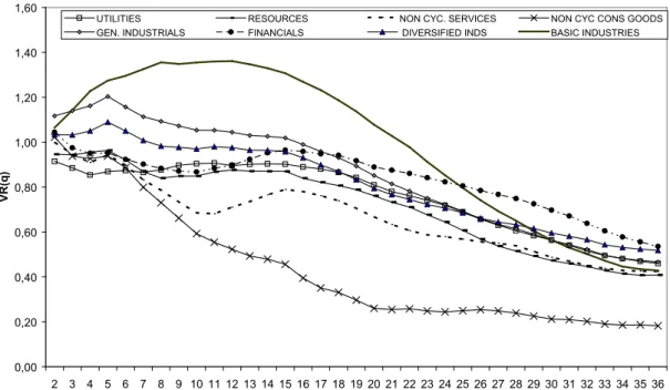
We present in Figure 1 the VR for the different sector indices for monthly returns. Basic in-dustries is highly persistent as the VR becomes less than one only after 22 months. Non cyclical consumer goods has a VR less than one for all investment horizons (q), except for 2 months. Ge-neral industries is also persistent if compared to other sectors (the VR becomes less than one only after 16 months). Non cyclical services is humped-shaped in the beginning but has a downward trend. Our results are in line with the findings of Poon (1996), which have found different patterns in the behavior of the VR for different sectors in the economy.7

figure 1 – variance ratios for different investment horizons

0,00 0,20 0,40 0,60 0,80 1,00 1,20 1,40 1,60

2 3 4 5 6 7 8 9 10 11 12 13 14 15 16 17 18 19 20 21 22 23 24 25 26 27 28 29 30 31 32 33 34 35 36

q

VR(q)

UTILITIES RESOURCES NON CYC. SERVICES NON CYC CONS GOODS GEN. INDUSTRIALS FINANCIALS DIVERSIFIED INDS BASIC INDUSTRIES

4 c

This paper empirically examined the RWH for the Brazilian stock market using a sector-based approach over the period 1994-2002. VR statistics with derived heteroscedasticity-consistent distributions using a weighted bootstrap method indicate that, with the exception of Basic Indus-tries, all sectors indices obey the RWH with weekly returns. This result is not robust to the use of monthly returns. Nonetheless, the dynamics in the VR seem to be different for some indices. While basic industries seem to be highly persistent, non cyclical consumer goods have a fairly high downward trend and seem mean reverting.

These are only two sectors for which there is weak evidence suggesting the rejection of the RWH. We can conclude that for most sector indices we can use the RWH to price assets and build financial models.

r

Ayadi, O. F.; Pyun, C. S. An application of variance ratio test to the Korean securities market. Journal of Banking and Finance 18, p. 643-658, 1994.

Blasco, N.; Rio, C. D.; Santamaria, R. The random walk hypothesis in the Spanish stock market: 1980-1992. 1997.

Cecchetti, S. G.; Lam, P. Variance ratio tests: small-sample properties with an application to international output data. Journal of Business and Economic Statistics 12, p. 177-186, 1994.

Cribari-Neto, F.; Zarkos, S. G. Bootstrap methods for heteroskedastic regression models: evidence on estimation and testing. Econometric Reviews 18, p. 211-228, 1999.

Darrat, A. F.; Zhing, M. On testing the random-walk hypothesis: a model-comparison approach. The Financial Review 35, p. 105-124, 2000.

Dockery, E.; Vergari, F. Testing the random walk hypothesis: evidence for the Budapest stock exchange.

applied Economic letters 4, p. 627-629, 1997.

Grieb, T.; Reyes, M. G. Random walk tests for Latin American equity indexes and individual firms. The Journal of Financial Research 22, p. 371-383, 1999.

Huang, B. Do Asian stocks market prices follow random walks? Evidence from the variance ratio test.

applied Financial Economics 5, p. 251-256, 1995.

International Finance Corporation (IFC). Emerging market fact book. Washington, DC: IFC, 1995. _______. Emerging market fact book. Washington, DC: IFC, 1999.

Lo, A. W.; MacKinlay, A. C. Stock market prices do not follow random walks: evidence from a simple specification test. The Review of Financial Studies 1, p. 41-66, 1988.

_______. The size and power of the variance ratio test in finite samples. Journal of Econometrics 40, p. 203-238, 1989.

Karamera, D.; Ojah, K.; Cole, J. A. Random walks and market efficiency tests: evidence from emerging equity markets. Review of Quantitative Finance and accounting 13, p. 171-188. 1999.

Malliaropulos, D.; Priestley, R. Mean reversion in Southeast Asian stock markets. Journal of Empirical Finance 6, p. 355-384, 1999.

Poon, S. Persistence and mean reversion in UK stock returns. European Financial Management 2, p. 169-196, 1996.

Urrutia, J. L. Tests of random walk and market efficiency for Latin American emerging equity markets.

The Journal of Financial Research 18, p. 299-309, 1995.

Wu, C. F. J. Jackknife, bootstrap and other resampling methods in regression analysis. annals of Statistics