Journal of Applied Fluid Mechanics, Vol. 8, No. 3, pp. 591- 600, 2015. Available online at www.jafmonline.net, ISSN 1735-3572, EISSN 1735-3645.
Ferromagnetic Liquid Flow due to Gravity
-
Aligned
Stretching of an Elastic Sheet
L. S. Rani Titus
1†and A. Abraham
21 Department of Mathematics, Jyoti Nivas College, Bangalore, India 2
Department of Mathematics, BMS Institute of Technology, Bangalore, India
†Corresponding Author Email: ranititus@gmail.com
(Received November 04, 2013; accepted August 02, 2014)
A
BSTRACTThe flow of a ferromagnetic liquid due to gravity-aligned stretching of an elastic sheet in the presence of a magnetic dipole is considered. The fluid momentum and thermal energy equations are formulated as a six parameter problem and a numerical study is made using the shooting method based on Runge – Kutta Fehlberg and Newton Raphson methods. Extensive computation on the velocity and temperature profiles is presented for a wide range of values of the parameters. It was found that the primary effect of the magnetothermomechanical interaction is to decelerate the fluid motion as compared to the hydrodynamic case. The results have possible industrial applications in ferromagnetic liquid based systems involving stretchable materials.
Keywords: Ferromagnetic liquid; Magnetic dipole; Stretching sheet; Grashof number; Prandtl number; Shooting method.
NOMENCLATURE
A, D positive constants f
C local skin friction coefficient cp specific heat at constant pressure
g acceleration due to gravity
Gr Grashof number
H magnetic field
K pyromagnetic coefficient k thermal conductivity L characteristic length
M magnetization
Pr Prandtl number T temperature of the fluid
Tw temperature of the stretching sheet Tc Curie temperature
(u,v) velocity along the x, y axes (U,V) nondimensional radial and axial
velocities
dimensionless distance from the origin to the center of the magnetic pole ferrohydrodynamic interactionparameter
thermal expansion coefficient
non-dimensional Curie temperatureӨ(ξ , η) nondimensional Temperature
viscous dissipation parameter μ dynamic viscosity
μ0 magnetic permeability kinematic viscosity
fluid density
shear stress at the sheet
magnetic scalar potential (ξ , η) nondimensional lengths1. INTRODUCTION
The study of laminar boundary layer flow and heat transfer in Newtonian and non-Newtonian fluids past a stretching sheet has been investigated extensively by many researchers due to its scientific and engineering applications. In processes such as polymer extrusion, the object on passing between two closely placed solid blocks is stretched into a liquid region. The desired mechanical properties of
the extrudate depends on the rate of cooling/heating and the rate of stretching (see Fisher E.G. 1976; Bailey R.L. 1983).
In the present problem the viscous and nonconducting ferrofluid is representative of the ambient liquid which serves the purpose of controlled heat transfer in the presence of a magnetic field.
of a carrier fluid and suspended particles. These particles are small (3-5 nm), solid, magnetic, single domain and coated with a molecular layer of a dispersant. Thermal agitation keeps them suspended and the coating keeps them noncolloidal (see Rosensweig R.E. 1985; Neuringer and Rosensweig 1964).
The combined influence of thermal and magnetic field gradients on the saturated ferrofluid flowing along a flat plate was investigated by NeuringerJ.L. (1966). The flow of a viscous fluid past a linearly stretching surface was considered by Crane L.J. (1970) for a Newtonian fluid. Andersson and Valnes (1998) extended Crane’s problem by studying the influence of the magnetic field, due to a magnetic dipole, on a shear driven motion (flow over a stretching sheet) of a viscous non-conducting ferrofluid. It was concluded that the primary effect of the magnetic field was to decelerate the fluid motion as compared to the hydrodynamic case. At the present time there are enumerable papers on the stretching sheet problem using different continua and considering various effects such as non-Newtonian characteristics, radiation, and magnetic field and so on. The above discussions can be found in Abel et al. 2008, 2009a, 2009b, 2009c, 2009d, 2011; Andersson 1998, 1992, 2006; Cortell 2010, 2008, 2007a, 2007b, 2006; Dandapat 2011, 2010, 2007; Dulal Pal 2010a, 2010b; Siddheshwar and Mahabaleshwar 2005; Hayat et al. 2010a, 2010b; Abbas et al.2010; Wang C.Y. 2007; Hamad 2007; Arnold et al. 2010; Seddeek 2007; Prasad et al. 2010; Magyari and Keller 2006; Van Gorder and Vajravelu 2010; Vajravelu and Cannon 2006; Abdoul and Ghotbi 2009; Tzirtzilakis and Kafoussias 2003 and the references there in. In many of the physical situation the sheet may be stretched vertically, rather than horizontally, into the ambient liquid. In this case the liquid flow and the heat transfer characteristics are determined by the motion of the stretching sheet and the buoyant force. There are no studies in literature concerning the flow and heat transfer in a ferrofluid due to a vertical stretching sheet in the presence of external magnetic field. This paper aims at studying the same using two different types of boundary heating, namely, prescribed surface temperature (PST) and prescribed surface heat flux (PHF). Shooting method based on Runge-Kutta-Fehlberg and Newton Raphson schemes is used in arriving at the numerical solution of the proposed problem.
2. MATHEMATICAL FORMULATION
Consider a steady two-dimensional flow of an incompressible, viscous and electrically non conducting ferrofluid driven by an impermeable sheet in the vertical direction. By applying two equal and opposite forces along the direction of gravity which is taken as the x-axis, and y-axis in a direction normal to the flow, the sheet is stretched with a velocity uw (x) which is proportional to the
distance from the origin. A magnetic dipole is located some distance from the sheet. The centre of
the dipole lies on the y-axis at a distance ‘a’ from the x-axis and whose magnetic field points in the positive x-direction giving rise to a magnetic field of sufficient strength to saturate the ferrofluid. The stretching sheet is kept at a fixed temperature Tw
below the Curie temperature Tc, while the fluid
elementsfar away from the sheet are assumed to be at temperature T = Tc and hence incapable of being
magnetized until they begin to cool upon entering the thermal boundary layer adjacent to the sheet. The boundary layer equations governing the flow and heat transfer in a ferrofluid are as follows,
0
u v
x y
(1)
2 0
2 (c )
u v u H
u v M g T T
x y y x
(2)
0
2 2
2
2 2
p
T T M H H
c u v T u v
x y T x y
T u v
k
y y y
(3)
where u and v are the velocity components along x and y directions respectively, is the fluid density,
the dynamic viscosity,
the kinematic
viscosity, Cp specific heat at constant pressure, k the thermal conductivity, g the acceleration due to gravity, representing the coefficient of thermal expansion, 0the magnetic permeability, M the magnetization, H the magnetic field, T the temperature of the fluid.
The assumed boundary conditions for solving the above equations are:
wu = cx , v = 0,
T = T in PST 0
in PHF
c
w
x
T A at y
L
T x
k q D
y L
(4)
0,
u T T as y
(5)
where k is the thermal conductivity of the fluid. A
and D are positive constants and L = c
2 2
2 ( )
x
x y a
, (6)where is the dipole moment per unit length. The magnetic field H has the components
2 2
2
2 2
( )
2 ( )
x
x y a
H
x x y a
(7)
2 2
22 ( )
2 ( )
y
x y a H
y x y a
(8)
Since the magnetic body force is proportional to the gradient of the magnitude of H, we obtain:
12 2 2 H x y
(9)
4 2 3 5 2 , 2 2 42 ( )
H x
x y a
H x
y y a y a
(10)Variation of magnetization M with temperature T is approximated by a linear equation
M = K ( Tc – T ) (11)
where K is the pyromagnetic coefficient.
3. SOLUTION PROCEDURE
We now introduce the non - dimensional variables as assumed by Andersson (1998).
1 2( , ) c ( , )x y
, ( ,U V) ( , )u v
c
, (12)
2
1 2
2
1 2
( ) ( ) in PST case ( , )
( ) ( ) in PHF case
c c w T T T T
(13)Where c w
x
T T A
L
in PST case,
c w
DL x
T T
k L
in PHF case.
The boundary layer equations 1-3 on using 10-13 takes the following form:
0
U V
(14)
2
2 2
4 1 2 1 2
2 2 4 U U U V U Gr
(15)
2 1 2 2' 2 '
2 1 2
2 5 4 3 2 2 '' '' 1 2 Pr 2
2 2 4
2
U V
U V V
U V (16)
The boundary conditions, given by Eq. (4), now takes the form:
1 2
' '
1 2
( , 0) , ( , 0) 0,
( , 0) 1, ( , 0) 0, (PST),
( , 0) 1, ( , 0) 0, (PHF),
( , ) 0, ( , ) 0
U V U
(17)Introducing the stream function
( , )
f( ) that satisfies the continuity equation in the dimensionless form 14, we obtain:'
( ), ( ),
U f V f
(18)
where the prime denotes differentiation with respect to . On using Eq. (10), Eq. (12) and Eq. (18) in Eq. (15) and Eq. (16), we obtain the following boundary value problem
(i) PST
' ' ' ' ' 2 1
1 4
' 2
( ) 0
( )
f ff f Gr
(19)
' ' ' '
1 1 1
2 1
3 Pr
2
( ) 2 ( ) 0,
( ) f f f f (20)
' ' ' 2 ' ' 2
2 2 2 3
'
1 4 5
2
( ) Pr(3 )
( )
2 4
( ) 0,
( ) ( )
f
f f f
f f
(21) ' 1 20, 1, 1, 0 at 0
f f (22)
'
0
f , 1 0, 2 0 as (23)
' ' ' ' ' 2 1
1 4
' 2
( ) 0
( )
f ff f Gr
(24)
' ' ' '
1 1 1
2
1 3
Pr
2
( ) 2 0
( ) f f f f (25)
' ' ' 2 ' ' 2
2 2 2 3
'
1 4 5
2
( ) Pr(3 )
( )
2 4
( ) 0
( ) ( )
f
f f f
f f
(26) ' ' ' 1 20, 1, 1, 0 at 0
f f (27)
'
1 2
0, 0, 0 as
f (28)
The six dimensionless parameters, which appear explicitly in the transformed problem, are the Prandtl number Pr, the viscous dissipation parameter , the dimensionless Curie temperature
, the ferrohydrodynamic interaction parameter , the Grashof number Gr and the dimensionless distance
from the origin to the center of the magnetic pole, defined respectively asPr p C k , 2 ( ) c w c
k T T
, c c w T T T , ' 0 2 ( ) 2 c w
K T T
, 2 g A Gr c L , 1 2 2 c a
(29)The local skin friction coefficient
f
C , which is a dimensionless form of the shear stress
at the sheet is given by:f C = 2 2 ( ) xy cx = 1 2
2f (0) Rex
(30)
In the PST case we are fixing the surface temperature and hence we calculate the local heat flux as follows,
1
2 2
1 2
Re [ (0) (0)]
x x
Nu
(31)In the PHF case we are fixing the surface heat flux and hence we compute the surface temperature as follows,
21 2
[ (0) (0)]
DL x
Tw Tc
k L
(32)
3.1 Method of Solution:
The three coupled differential equations (19) to (21) subject to the boundary conditions (22) and (23) constitute a non - linear two - point boundary value problem, which is solved by means of a standard shooting technique. The higher order ordinary differential equations are formulated as first order equations and the resulting set of seven first order equations can be integrated as an initial value problem using the adaptive stepping Runge-Kutta- Fehlberg (RKF45) method. The trial values of
'' ' '
1 2
(0), (0), (0)
f were adjusted iteratively
by Newton Raphson‘s method to assure a quadratic convergence of the iterations required in order to fulfill the right end boundary conditions. The initial value problem to be solved are given below
3.2 Initial Value Problem-1 (IVP-1)
1 2 2 3 2 3 4
2 1 3 4 4
4
5
2
5 1 4
1 5 3 2
6
7
2
7 1 6
3 1 7 2 6 3
2 1
4 4 5
, , 2 , ( ) ,
2 ( )
Pr 2 ,
( )
,
2
Pr( 2 )
( ) 2 4 ( ) , ( ) ( ) dy y dx dy y dx dy y
y y y Gr y
dx
dy y dx
dy y y
y y y
dx
dy y dx
dy y y
y y y y y
dx y y y
(33) with the initial conditions:y1(0)=0, y2(0) = 1, y3(0) = a0, y4(0) = 1,
y5(0) = b, y6(0) = 0, y7(0) = c0 (34)
We need to solve a sequence of initial value problems as above so that the end boundary values thus obtained numerically match upto a desired degree of tolerance with the boundary values at
given in the problem. Now the problem is to find a0,b0, c0 such that:
F1 (a0, b0, c0) = f (, a0, b0, c0) –
f() = y2 (, a0, b0, c0) – y2 (),
F2 (a0, b0, c0) =
1 (, a0, b0, c0) – 1F3 (a0, b0, c0) =2 (, a0, b0, c0) –
2
(
) = y6 (, a0, b0, c0) – y6 (). (35)These are three nonlinear equations in a, b, and c which are solved by the Newton-Raphson method. This method for finding roots of non-linear equations, with a0, b0 and c0 as the initial values,
yields the following iterative scheme:
( ,, ) 1
1 1 1
1 1
2 2 2
1 2
3 1
3 3 3
( , , )
abc nnn
n n n
n n
n n
n n
a b c
F F F
a b c
a a F
F F F
b b F
a b c
F
c c
F F F
a b c
,
(n = 0, 1, 2, ...). (36) To implement Newton-Raphson method, the nine partial derivatives of F1, F2 and F3 with respect to a,
b and c are required. By differentiating the IVP 1 of Eq. (33) and Eq. (34), with respect to a and setting
Yi =
i
y
a
, the second initial value problem (IVP-2)
is obtained.
3.3 Initial Value Problem-2 (IVP-2)
1
2
2
3
3 4
22 1 3 1 3 4 4
4
5
5
1 5 1 5 3 1 4 1 4
2 2
6
7
7
3 3 1 7 1 7 2 6 2 6
2 1
1 6 1 6 4
3 4 5
2 2
( )
2
Pr Pr ( )
( )
4
2 Pr 2 2
2 4
2
( ) ( ) ( )
dY Y dx dY
Y dx
dY Y
y Y y Y Y y GrY dx
dY Y dx
dY
y Y Y y Y y y Y
dx
y Y
dY Y dx dY
y Y Y y y Y y Y Y y dx
y y
y Y Y y Y
x x
2 1
4 4 5
2 4
( )
( ) ( )
Y Y
y
x x
(37)
with the initial conditions,
Y1 (0) = 0; Y2 (0) = 0; Y3 (0) = 1; Y4 (0) = 0;
Y5 (0) = 0; Y6 (0) = 0; Y7 (0) = 0. (38)
Similarly IVP-3, IVP-4 are obtained by differentiating IVP-1 with respect to b and c respectively. Thus three additional initial value problems IVP-2, IVP-3 and IVP-4 known as the variational equations in literature, are obtained and solved using variable stepping RKF45 method.
4. RESULTS AND DISCUSSION
An analysis is carried out to study the effect of magnetic field on the flow of the ferromagnetic liquid due to a vertically stretched sheet. Heat transfer is studied using two different boundary heating, namely, PST and PHF. With the aid of similarity transformations the partial differential equations governing the flow and heat transfer are converted into a set of non-linear coupled ordinary differential equations. The resulting problem is a boundary value one and the same is solved using shooting technique based on RKF45 and NR methods. The numerical results are shown in the form of graphs from Figs. 2 to 7. The skin friction coefficient is tabulated in Table 1 for a wide range of values of the governing parameters.
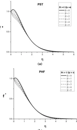
Figure (2) shows the effect of ferrohydrodynamic interaction parameter on velocity profiles '
( )
f for PST and PHF cases. From these plots it is evident that increasing values of results in flattening of '
( )
f . The transverse contraction of the velocity boundary layer is due to the applied magnetic field, which produces considerable opposition to the motion.
Fig. 1. Schematic representation of flow configuration (broken lines represent the
(a)
(b)
Fig. 2. Effect of ferrohydrodynamic interaction parameter
on velocity profile in PST andPHF with
= 1,
= 2 and
= 0.01(a)
(b)
Fig. 3. Effect of Prandtl number Pr on velocity profile in PST and PHF with
= 1,
= 2 and
= 0.01(a)
(b)
Fig. 4. Effect of Grashof number Gr on velocity profile in PST and PHF
= 1,
= 2 and
= 0.01(a)
(b)
Fig. 5. Effect of ferrohydrodynamic interaction parameter
on temperature profile in PST and(a)
(b)
Fig. 6. Effect of Prandtl number Pr on temperature profile in PST and PHF with
=1,
= 2 and
= 0.01(a)
(b)
Fig. 7. Effect of Grashof number Gr on temperature profile in PST and PHF with
=1,
= 2 and
= 0.01(a)
(b)
(c)
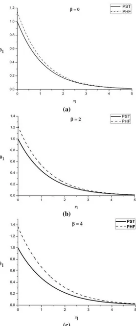
Fig. 8. Comparison of heat transfer in two boundary conditions PST and PHF when is
varied with
= 1,
= 2 and
= 0.01From Fig. 3 which illustrates the effect of Pr on the velocity profiles it is clear that increasing values of Pr reduces the horizontal velocity profiles in both PST and PHF cases. The Prandtl number is the ratio of two diffusivities, diffusivity of momentum and vorticity and that of the heat. At high Prandtl number the fluid is very viscous and the velocity is reduced.
accelerating the fluid in the boundary layer region. It also indicates the relative importance of inertia to viscous forces. When Gr is large the domination of advection over conduction always occurs simultaneously with dominance of inertial forces over viscous forces. It can also be interpreted as that the flow will have a boundary layer character. Figure (5) shows the effect of on temperature profiles. As increases the skin friction is increased which enhances the heat transfer. The same effect is reiterated in Fig. 5. A number of striking phenomena are exhibited by the magnetic fluid in response to the impressed magnetic fields. These responses include the normal field instability due to which a pattern of spikes appears on the fluid surface, enhanced convective cooling in ferrofluids having a temperature dependent magnetic moment, unusual buoyancy relationships, such as the self-levitation of an immersed magnet. The parameter
has a regulating effect on the fluid as it regulates
the velocity of the motion. This happens only at the lower values of , but at higher values some unrealistic patterns are observed.
Figure (6) highlights the effect of thermal diffusivity parameter Pr on heat transfer. It is clear from this figure that the fluid with lesser Prandtl number is effective in controlling the heat transfer. The effect of Grashof number on heat transfer is same as that of Pr as can be seen from Fig. 7. Here we note that for Gr = 0 recovers the results of horizontal stretching sheet problem.
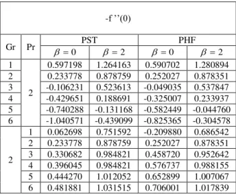
The skin friction coefficient is tabulated in Table 1 for various values of , Pr and Gr. This table highlights the same effects of the parameters that we have discussed through figures. The skin friction is increased in presence of magnetic field ( = 2) as compared to the case of absence of magnetic field ( = 0) that is, dominates in controlling the heat transfer as compared to other parameters.
Table 1 Values of -
f
''(0)
for different values of Gr and Pr in the absence / presence of ferromagnetismfor PST and PHF
-f ’’(0)
Gr Pr PST PHF
0
2 0 2 1
2
0.597198 1.264163 0.590702 1.280894
2 0.233778 0.878759 0.252027 0.878351
3 -0.106231 0.523613 -0.049035 0.537847 4 -0.429651 0.188691 -0.325007 0.233937 5 -0.740288 -0.131168 -0.582449 -0.044760 6 -1.040571 -0.439099 -0.825365 -0.304578
2
1 0.062698 0.751592 -0.209880 0.686542 2 0.233778 0.878759 0.252027 0.878351 3 0.330682 0.984821 0.458720 0.952642 4 0.396045 0.984821 0.576737 0.988155 5 0.444270 1.012052 0.652899 1.007067 6 0.481881 1.031515 0.706001 1.017839
From the Fig. 8 it is clear that the thermal boundary layer thickness in PHF case exceeds the PST case showing that more heat is diffused away into the system. Hence the PHF boundary conditions are better suited for proper cooling of the sheet. As mentioned earlier the desired properties of the extrudate depend on the rate of cooling. For applications where in the better cooling rate is required the PHF boundary condition can be made use.
5. CONCLUSIONS
The following inference is arrived at from the results that we have discussed in the previous section.
1. The ferrohydrodynamic interaction parameter has a significant say in the control of flow and heat transfer of the ferrofluid. It should be kept at minimum.
2. Grashof and Prandtl numbers assists flow thereby reducing heat transfer hence these parameters als must be at their minimum for effective cooling.
ACKNOWLEDGEMENTS
The authors would like to thank their respective Institutions for their support.
REFERENCES
Abbas, Z., Y. Wang, T. Hayat, and M. Oberlack (2010). Mixed convection in thestagnation-point flow of a Maxwell fluid towards a vertical stretching surface. NonlinearAnalysis: Real World Applications 11(4), 3218-3228. Abel, M. S., and N. Mahesha (2008). Heat transfer
non-uniform heat source and radiation. Applied Mathematical Modelling 32, 1965-1983. Abel, M. S., P. G. Siddheshwar, and N. Mahesha
(2009a). Effects of thermal buoyancy and variable thermal conductivity on the MHDflow and heat transfer in a power-law fluid past a vertical stretching sheet in the presence of a non - uniform heat source. Int. J. Non - linear Mech. 44, 1-12.
Abel, M. S., M. Mahantesh, and M. M. Nandeppanavar (2009b). Heat transfer in MHD viscoelastic boundary Layer flow over a stretching sheet with non-uniform heat source/sink. Communications in Nonlinear Science and Numerical Simulation 14(5), 2120-2131.
Abel, M. S., P. S. Datti, and N. Mahesha (2009c). Flow and heat transfer in a power-law fluid over a stretching sheet with variable thermal conductivity and non-uniform heat source. I. J. of Heat and mass Transfer 52, 2902-2913. Abel, M. S., N. Mahesha, and J. Tawade (2009d).
Heat transfer in a liquid film over an unsteady stretching surface with viscous dissipation in presence of external magnetic field. Applied Mathematical Modelling 33, 3430-3441. Abel, M. S., P. G. Siddheshwar, and N. Mahesha
(2011). Numerical solution of the momentum and Heat transfer equations for a hydromagnetic flow due to a stretching sheet of a non - uniform property micro polar liquid.
Applied Mathematics and computation 217, 5895-5909.
Andersson, H. I. (1992). MHD flow of a viscoelastic fluid past a stretching surface.
Acta Mech. 95, 227-230.
Andersson, H. I., and O. A. Valnes (1998). Flow of a heated Ferrofluid over a stretching sheet in the presence of a magnetic dipole. Acta Mechanica 128, 39-47.
Andersson H. I. (2002). Slip flow past a stretching surface. Acta Mech. 158, 121.
Andersson, H. I., and V. Kumaran (2006). On sheetdriven motion of power-law fluids.
International Journal of Non-Linear
Mechanics 41(10), 1228-1234.
Arnold, J., A. Asir, S. Somasundaram, and T. Christopher (2010). Heat transfer in a viscoelastic boundary layer flow over a stretching sheet. Int. J. of Heat and Mass Transfer 53(5), 1112-1118.
Bailey, R. L., (1983). Lesser known applications of Ferrofluids. J. Magnetism Magn. Mater 39, 178-182.
Cortell, R. (2006). Flow and heat transfer of an electrically conducing fluid of second grade over a stretching sheet subject to suction and to a transverse magnetic field. Int. J. Heat and Mass Transfer 49, 1851-1856.
Cortell, R. (2007a). Viscoelastic fluid flow and heat transfer over a stretching sheet under the effects of a non-uniform heat source, viscous dissipation and thermal radiation. Int. J. Heat and Mass Transfer 50 (15-16), 3152-3162. Cortell, R. (2007b). Viscous flow and heat transfer
over a nonlinearly stretching sheet. Appl. Math.Comput. 184 (2), 864-873.
Cortell, R. (2008). Similarity solutions for flow and heat transfer of a quiescent fluid over a
nonlinearly stretching sheet.
J.Mater.Process.Technol. 203 (1-3), 176-183. Cortell, R. (2010). On a certain boundary value
problem arising in shrinking sheet flows.
Applied Mathematics and Computation 217 (8), 4086-4093.
Crane, L. J. (1970). Flow past a stretching plate. J. Appl. Math. Phys. (ZAMP) 21, 645- 647. Dandapat, B. S., B. Santra, and K. Vajravelu
(2007). The effects of variable fluid properties and thermocapillarity on the flow of a thin film on an unsteady stretching sheet. International Journal of Heat and Mass Transfer 50 (5-6), 991-996.
Dandapat, B. S., and S. Chakraborty (2010). Effects of variable fluid properties on unsteady thin-film flow over a non-linear stretching sheet.
International Journal of Heat and Mass Transfer 53 (25-26), 5757-5763.
Dandapat, B. S., and S. K. Singh (2011). Thin film flow over a heated nonlinear stretching sheet in presence of uniform transverse magnetic field.
International Communications in Heat and Mass Transfer 38 (3), 324-328.
Fisher, E. G. (1976). Extrusion of Plastics, 3rd ed., London: Newnes-Butterworld.
Ghotbi, A. R. (2009). Homotopy analysis method for solving the MHD flow over a non-linear stretching sheet. Communications in Nonlinear Science and Numerical Simulation 14(6), 2653-2663.
Hamad, M. A. A. (2007). Analytical solution of natural convection flow of a nanofluid over a linearly stretching sheet in the presence of magnetic field. International Communications in Heat and Mass Transfer 38 (4), 487-492. Hayat, T., M. Mustafa, and I. Pop (2010a). Heat and
mass transfer for Soret and Dufour’s effect on mixed convection boundary layer flow over a stretching vertical surface in a porous medium filled with a viscoelastic fluid.
Communications in Nonlinear Science and Numerical Simulation 15 (5), 1183-1196. Hayat, T., Z. Abbas, I. Pop, and S. Asghar (2010b).
Effects of radiation and magnetic field on the mixed convection stagnation-point flow over a vertical stretching sheet in a porous medium.
Magyari, E., and B. Keller (2006). Heat transfer characteristics of boundary-layer flows induced by continuous surfaces stretched with prescribed skin friction. Heat Mass Transfer
42 (8), 679-687.
Neuringer, J. L., and R. E. Rosensweig (1964). Ferrohydrodynamics. Phys. Fluids 7, 1927-1937.
Neuringer, J. L. (1966). Some viscous flows of a saturated ferrofluid under the combined influence of thermal and magnetic field gradients. Int. J. Non - linear Mech. 1, 123-127.
Pal, D., and B. Talukdar (2010a). Perturbation analysis of unsteady magnetohydrodynamic convective heat and mass transfer in a boundary layer slip flow past a vertical permeable plate with thermal radiation and chemical reaction. Communications in Nonlinear Science and Numerical Simulation
15 (7), 1813-1830.
Pal, D. (2010b). Mixed convection heat transfer in the boundary layers on an exponentially stretching surface with magnetic field. Applied Mathematics and Computation 217 (6), 2356-2369.
Prasad, K. V., P. S. Datti, and K. Vajravelu (2010). Hydromagnetic flow and heat transfer of a non- Newtonian power law fluid over a vertical stretching sheet. Int. J. of Heat and Mass transfer 53 (5-6), 879-888.
Rosensweig R. E. (1985). Ferrohydrodynamics, 1st ed., New York: Cambridge University Press. Seddeek, M.A. (2007). Heat and mass transfer on a
stretching sheet with a magnetic field in a Visco-elastic fluid flow through a porous medium with heat source or sink.
Computational Materials Science 38 (4), 781-787.
Siddheshwar, P. G., and U. S. Mahabaleshwar (2005). Effect of radiation and heat source on MHD flow of a viscoelastic liquid and heat transfer over a stretching sheet. Int. J. Non-Linear Mech. 40, 807-820.
Tzirtzilakis, E. E., and N. G. Kafoussias (2003). Biomagnetic fluid flow over a stretching sheet with non-Linear Temperature dependant magnetization. ZAMP 54, 551-565.
Vajravelu, K., and J. R. Cannon (2006). Fluid flow over a nonlinearly stretching sheet. Applied Mathematics and Computation 181 (1), 609-618.
Vangorder, R. A., and K. Vajravelu (2010). Hydromagnetic stagnation point flow of a second grade fluid over a stretching sheet.
Mechanics Research Communications 37 (1), 113-118.