Artigo
*e-mail: [email protected]
TIME-SERIES FORECASTING OF POLLUTANT CONCENTRATION LEVELS USING PARTICLE SWARM OPTIMIZATION AND ARTIFICIAL NEURAL NETWORKS
Francisco S. de Albuquerque Filho, Francisco Madeiro e Sérgio M. M. Fernandes
Centro de Ciências e Tecnologia, Universidade Católica de Pernambuco, Boa Vista, 50050-900 Recife - PE, Brasil
Paulo S. G. de Mattos Neto*
Centro de Informática, Universidade Federal de Pernambuco, 50740-560 Recife - PE, Brasil
Tiago A. E. Ferreira
Departamento de Estatística e Informática, Universidade Federal Rural de Pernambuco, 52171-900 Recife - PE, Brasil
Recebido em 1/8/12; aceito em 8/2/13; publicado na web em 4/6/13
This study evaluates the application of an intelligent hybrid system for time-series forecasting of atmospheric pollutant concentration levels. The proposed method consists of an artificial neural network combined with a particle swarm optimization algorithm. The method not only searches relevant time lags for the correct characterization of the time series, but also determines the best neural network architecture. An experimental analysis is performed using four real time series and the results are shown in terms of six performance measures. The experimental results demonstrate that the proposed methodology achieves a fair prediction of the presented pollutant time series by using compact networks.
Keywords: particle swarm optimization; artificial neural networks; pollutants’ concentration time series.
INTRODUCTION
Pollution is one of the most relevant problems of metropolitan areas. With population growth and economical increases leading to new industry, environmental health problems have captured society’s interest. Problems that affect the ecosystem, such as noise pollution; garbage and its disposal; and, in particular, air pollution, have a direct effect on people’s health.1,2
There are numerous air quality indicators that show pollution effects on people’s health.1,2 Some of the most important ones inclu-de particulate matter (PM10), carbon monoxide (CO), sulfur dioxide (SO2), and nitrogen dioxide (NO2). When an indicator’s concentration level exceeds an established air quality safety threshold, severe he-alth problems may affect humans.1,2 There are many environmental agencies around the globe that develop their own policies and have established air quality standards and indicators regarding allowed atmospheric pollutant levels. Environmental agencies use the indi-cators as a monitoring measure, using a network of pollution and atmospheric sensors. The measurement results are observations equally spaced and ordered in time (e.g., hourly, daily, and monthly), resulting in a time series of pollutant concentrations.
Methods used for time-series prediction are native to the statistics field, such as the autoregressive (AR) model and the autoregressive moving average (ARMA) model.3,4 Various intelligent models, such as artificial neural networks (ANNs),5,6 particle swarm optimization (PSO),7-10 genetic algorithms,11 and fuzzy logic,12-13 have been proposed.
In the forecasting field, particularly for air pollution proble-ms,6,7,11,14-18 ANNs have been successfully applied.6,15 Brunelli used a recurrent neural network (Elman model) to predict daily maximum concentrations of SO2, O3, PM10, NO2, and CO in the city of Palermo.6 Kurt et al.applied a feed forward ANN trained by back propagation with seven nodes in the input layer and ten nodes in the hidden layer to predict three air pollution indicator (SO2, PM10, and CO) levels for the next three days for districts in the greater Istanbul area.15
However, use of an ANN requires the choice of a set of parameters
and an appropriate architecture for the problem solution. Intelligent hybrid models7,9-13,16,18-19 that are a combination of different intelligent methods are proposed with the aim of achieving better prediction performance, with the intent of combining the strong points of several algorithms into a single system. There are some studies in the literatu-re that use these ideas, wheliteratu-re an intelligent search method is combined with an ANN to enhance a predictive system. Lu et al. combined a PSO model with an ANN to predict pollutant levels in the downtown area of Hong Kong.7 Wang and Lu proposed a multilayer perceptron (MLP) model trained by a PSO algorithm, andapplied the hybrid approach for one step ahead (1-day) forecasting for daily maximum ozone (O3) levels in the Tsuen Wan and Tung Chung areas.16 Grivas and Chaloulakou used an optimization procedure based on a genetic algorithm for the selection of input variables for ANN models,17 and used the system for prediction of PM10 hourly concentrations in the greater Athens area.
The focus of this study is to employ a PSO algorithm for tuning and training an ANN. The resulting model is applied to time-series forecasting. On the basis of the authors’ knowledge of research literature, PSO has not been extensively used to predict time series of gaseous pollutants. In addition, a novelty of this study is the use of PSO to not only reach the relevant lags used in the prediction, but also to determine the best neural network architecture to forecast pollutant concentration levels.
TIME SERIES
A time series is a set of observations of a variable of interest, representing a sequence of observations ordered in time. The variable is observed in discrete temporal points, usually equally spaced, and the analysis of such temporal behavior involves a description of the process or of the phenomenon that generated the sequence.3,20 A time series can be defined by Equation 1,
Therefore, Xt is a sequence of observations ordered and equally spaced in time. The application of forecasting techniques relies on the ability to identify underlying regular patterns in the dataset that make it possible to create a model capable of generating subsequent temporal patterns.3,20
A crucial point regarding the time-series prediction problem is to capture the temporal relationship of the given series data. Hence, through observation of the correct time lags, the dynamics that gene-rated the real series can be reconstructed. This hypothesis is based on Takens theorem,21 which indicates that such reconstruction is possible. However, a major problem is the correct choice of relevant time lags. Therefore, the methodology used in this study is based on the search for the relevant time lags that provide a correct characterization of the process that governs a temporal series.9,19
ARTIFICIAL NEURAL NETWORKS
ANNs are computational modeling tools that find a wide variety of applications in modeling complex real-world problems.5,22 ANNs can be defined as structures composed of simple, adaptive, and mas-sively interconnected processing elements (referred to as artificial neurons or nodes) that are capable of performing data processing and knowledge representation.
A single neuron, or perceptron, shown in Figure 1, has two basic components. First, a weighted sum, s = Σni=1wixi + b of the inputs x1, x2, x3, …, xn, is calculated, where wiis the respective weight (synaptic weight) of the input xi and b is the bias of the neuron. Second, an activation function f(s) gives an output according to the result of s. A range of functions can assume the role of an activation function, including sigmoid, linear, and hyperbolic tangent functions.
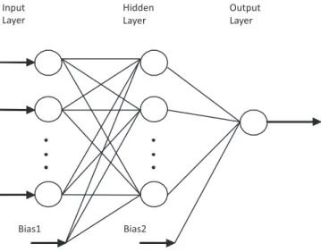
A multilayer neural network or MLP consists of two or more layers, as follows: input layer, hidden layer(s), and output layer (Figure 2). When formed by two layers, it only possesses the input layer and the output layer. Each node in the input layer receives a unique input signal. Actually, the nodes in this layer are usually passive, meaning they do not process data, but only receive signals on their input and send them to the nodes in the next layer.5,22 When the network is formed by three or more layers, the layer(s) between the input and output layers is(are) denominated hidden layer(s). A hidden layer processes the signals sent to it by calculating a weighted summation and using a specific activation function. Then, the output layer receives the signals from the previous layer by performing a weighted summation and applying a particular activation function to the resultant sum.
In this study, the neural networks used have the sigmoid function
and the linear function as the activation functions of the hidden and output layers, respectively.
The dataset used for training, validating, and testing the neural network is divided into three groups. First, the training set, which usually consists of half or more of all data gathered. It is used by the ANN to adjust its weights and biases. Second is the validation set, which is used for validating the network training. It checks the network’s capability to generalize a series of input data. Finally, the test set is used to evaluate the network’s performance.5 The latter two sets consist of data that have not been previously presented to the network.
The training process is performed until any stop criterion is achieved. The errors associated with the stop criteria are the validation (generalization) and training errors. The test error is the network’s performance measurement based on the test set. The training, valida-tion, and test errors are evaluated by comparing the actual observed data to the predicted data.
PARTICLE SWARM OPTIMIZATION
The PSO algorithm was developed by Eberhart and Kennedy in 1995.8 It is an evolutionary algorithm inspired by the behavior of flocks of birds or schools of fish searching for food. The algorithm seeks to optimize a population of random solutions. Each particle (individual) has a position and velocity, representing the solution to the optimization problem and the direction of the search in the search space. Particles adjust speed and position according to their best experiences. The algorithm determines the local best found by each particle individually and the global best, which is known by the entire swarm.
The PSO theory assumes that in a population with size M, each individual i, where 1 ≤I≤M, has a present position Xi, an associated velocity Vi, and a local best solution li In addition, each particle has a fitness function, which is the particle’s measure of merit and evalua-tes the particle’s solution adequacy in solving a given problem. The particle local best is simply the best solution obtained by it up to the current iteration. The global best solution Xg is the best solution among all the particles. Parameters c1 and c2 are the acceleration constants of the particles, and influence the velocity at which the particles move in the search space. For each iteration cycle, the particle velocities are updated (accelerated) in the direction leading to the local and global minima:
Vi(t) = wVi(t – 1) + c1r1(li – Xi(t)) + c2r2(Xg – Xi(t)) (2)
Figure 1. A single model of a neuron
The particles’ positions are updated using simple discrete dynamics:
Xi(t) = Xi(t –1) + Vi(t), (3)
where the term w is the inertia weight, and is used to balance the local and global search abilities of the algorithm, controlling the influence of previous information when updating the new velocity. Usually, the term w decreases linearly from 1 to approximately 0 during the process.7 The parameters r
1 and r2 are generated from a uniform random sequence in the interval [0, 1].
In the PSO algorithm, each individual in the population evolves according to its own experience, estimating its own quality. Since the individuals are social beings, they also exchange information with their neighbors. These two types of information correspond to indivi-dual learning (cognitive: local knowledge) and cultural transmission (social: knowledge of the best position in the swarm), respectively. The algorithm is formulated as follows:8
1. Initialize parameters such as the acceleration constants, inertia weight, number of particles, maximum number of iterations, velocity boundaries, initial and constrained velocities and posi-tions, and eventually the error limit for the fitness function. 2. Evaluate the particles’ fitness function values, comparing with
each other, therefore setting the local best and global best. 3. In accordance with Equations (2) and (3), calculate a particle’s
new speed and position, and then update each particle.
4. For each particle, compare the current fitness value with the local best. If the current value is better, update the local best fitness value and particle position with the current one.
5. For each particle, compare the current fitness value with the global best. If the current value is better, update the global best fitness value and particle position with the current one.
6. If a stop criterion is achieved, then stop the procedure, and output the results. Otherwise, return to step 2.
PROPOSED METHOD
This section describes the specifics for each of the models pro-posed in this study.
PSO is used to find the best possible MLP structure (input and hidden layers’ size) and to train the MLP characteristics (weights and biases). The following remarks are necessary to understand how PSO is employed to train the MLP model using Equations (2) and (3): • One MLP neural network corresponds to one particle in PSO
(with position and velocity properties). The components of each particle include the network structure (input and hidden layer sizes), the weights matrix, and the biases (hidden and output layers).
• The number of particles, in other words, the population size, de-fines how many MLPs will be used to search the optimal network and its characteristics.
• All MLP individual characteristics (weights, bias, and structure) are updated serially during the search process for the optimal solution. Updates are made on the basis of Equations (2) and (3). The proposed hybrid system combines two intelligent techniques, PSO and ANNs. The idea is that each individual of the population, which is an ANN, is adjusted and has its structure dimensioned by PSO. Therefore, PSO will determine the following:
• The maximum number of time lags (MAX_LAGS). PSO searches in the interval [1, MAX_LAGS] for the relevant lags that better characterize the time series for each individual of the population. • The number of hidden neurons; initially, a maximum number of
neurons (MAX_NHIDDEN), so that PSO can search in the interval
[1, MAX_NHIDDEN] for the optimum number of hidden neurons for each individual of the population.
With this methodology, it is possible to minimize the search time to determine the most compact network structure capable of representing the data.
PSO, when calculating new velocities and positions, uses those values to update the number of units in the input layer, the number of neurons in the hidden layer, the weights (of the hidden and output layers), and the biases (of the hidden and output layers). In this study, four combinations of the PSO algorithm with MLP ANNs are explored.
PSO updates the parameters within these models. Then, a ne-twork simulation is conducted to evaluate the nene-twork’s adequacy using the fitness function shown in Equation 4. This process is ended if any stopping criterion is reached. The model variations are as follows:
In the first two models, only PSO updates the network’s archi-tecture, and weights and biases matrices:
1. PSO-MLP: The PSO algorithm adjusts the ANN parameters, where the input lags are time window observations.
2. PSO-MLP with nonconsecutive lags (NCL): The PSO algorithm has the ability to choose a nonconsecutive sequence of time lags. This characteristic is applied to achieve a more compact network structure, thus leading to lower computational costs.
In the last two models, the PSO and the Levenberg–Marquardt (LM) gradient descent algorithm are used to adjust network archi-tecture and weights and bias matrices.
3. PSO-MLP-LM: At each predetermined stage in the algorithm (e.g, every 100 iterations), or at a stagnation point (e.g, when PSO is no longer able to enhance its prediction), the MLP trains the network. Training is also performed by the LM in an attempt to avoid stagnation.
4. PSO-MLP-LM with NCL: This model has two abilities. The first is it can choose a non-consecutive sequence of time lags and the second is the use of the LM in order to try to avoid stagnation. The PSO individuals are evaluated by the following fitness function:
. (4)
The fitness function is used to evaluate the model’s performance. In this study, more adapted PSO individuals have higher fitness values, approaching a value of 1.
The termination conditions for PSO are as follows: • The maximum number of PSO iterations (100) • The size of the population (swarm) reaches 60 particles • Training process error below 10−4
The stop criteria for the neural network training algorithm (LM) in this study are as follows:
• Maximum number of iterations (1000)
• Validation or generalization error greater than 5%
PERFORMANCE MEASURES
For the problem of tiseries forecasting, there is no single me-tric universally adopted by researchers to evaluate a model’s predictive adequacy. In the present study, six metrics are considered to allow a better appreciation of the forecasting system performance.6,9,19 First is the mean square error (MSE), which is one of the most common performance measures applied to neural networks:14
where n is the number of patterns, targetj is the desired output (series real value) for the j-th pattern, and outputj (model response) is the predicted value for the j-th pattern.
The second relevant measure is Theil’s U statistic, which com-pares the performance of the predictive model with a random-walk (RW) model. An RW model assumes that the most adequate value for the prediction at time t + 1 is the value obtained at time plus a noise term.19 If the Theil’s U statistic value is less than 1, then the model is better than RW; otherwise, the model has performance equal to or worse than RW (Theil’s U statistic value equal to or greater than 1, respectively).
. (6)
The third relevant evaluation measure, the average relative va-riance (ARV), is given by
, (7)
which compares the model performance with the time-series ave-rage, which is represented by the term —target. If ARV equals 1, the model has a performance similar to the time-series average. If ARV is greater than 1, then the model has a performance worse than the time-series average, and if ARV is less than 1, then the model has a better performance than the time-series average.
Another performance measure is the mean absolute percentage error (MAPE), given by
. (8)
Another important measure is the index of agreement (IA), which can express the difference between the observed and forecasted data. This index can range from 0 to 1. Higher values indicate a better adequacy to the prediction problem. The IA is given as
. (9)
The last performance measure is the prediction of change in direc-tion (POCID), which maps the time-series tendency; in other words, the model’s capability of predicting if future values will increase or decrease. The measure is formulated as follows:
, (10)
where
The fitness function considers the MSE. Nevertheless, the algorithm is also evaluated with the other five metrics discussed above. In a perfect system, all performance measures must appro-ach zero, except the POCID, which must approappro-ach 100; the IA,
which must approach 1; and the fitness function, which also must approach 1.
SIMULATION AND RESULTS
In this study, the following four real-world time series, corre-sponding to natural phenomena, were considered: gaseous concentra-tions of CO, SO2, NO2, and PM10. The data were taken from the city of São Caetano, located in the state of São Paulo, Brazil, and were obtained by CETESB-SP (Environmental Company of the State of São Paulo).23 The series were normalized to the interval [0,1] and divided into three groups, following the Proben 1 technical report:24 training set with 50% of the time-series data, validation set with another 25% of the time-series data, and test set with the remaining 25% of the time-series data. The PSO parameters were the same for all experiments. The number of iterations was 1000, and parameters c1 and c2 were established as 1.8 and 1.5, respectively. Terms r1 and r2 were random numbers between [0, 1].
Ten particles were used, in which each PSO individual was an ANN with maximum architecture of 10 – 10 – 1, which makes refe-rence to an MLP network, which denotes 10 units in the input layer, 10 units in the hidden layer, and 1 unit in the output layer (prediction horizon of one step forward). For each time series, 10 experiments were performed with the combined algorithms, where each algorithm with the greatest fitness function was chosen as the representative of the respective model for a particular time series.
In the next subsections, the experimental results achieved for the four time series are shown. For each time series, the data considered in the present paper correspond to the measured daily averages.
Carbon monoxide series
The measurements available for the CO pollutant were collected between the years 2000 and 2001. The dataset consists of 713 daily observations.
The best MLP structure was chosen after conducting 10 experi-ments for all four models. According to Table 1, the most adequate model was PSO-MLP-NCL. Among all metrics, PSO-MLP-NCL exhibited a superior performance based on the calculated MSE, POCID, MAPE, and IA. The selected architecture consists of a win-dow of two nonconsecutive time lags, 1 and 6. Thus, it has 2 units in the input layer and 10 units in the hidden layer. Therefore, the MLP architecture that best fits the problem was defined as 2 – 10 – 1.
Figure 3 represents the model’s prediction (dashed line) and ob-served data (solid line) for the CO series for the last 100 consecutive points in the test set.
Sulfur dioxide series
The values of the SO2 pollutant time series consisted of daily averages between the years 2000 and 2001. The series consisted of 699 observations.
Each model was submitted to 10 experiments. According to Table 2, PSO-MLP-LM obtained a superior performance when compared to the other proposed models in terms of MSE and IA. When compared to PSO-MLP-LM-NCL, PSO-MLP-LM was better in terms of MSE, POCID, MAPE, and IA.
The best model had a temporal window of three inputs, that is, time lags 1, 2, and 3, and the hidden layer had 9 processing units. Therefore, the selected architecture was 3 – 9 – 1.
average. In IA terms, all proposed models obtain similar perfor-mance. Figure 4 shows the PSO-MLP-LM prediction (dashed line) and observed data (solid line) for the SO2 series for the last 100 consecutive points.
Particulate matter series
The PM10 series is represented by 716 daily observations in the period between the years 2002 and 2003.
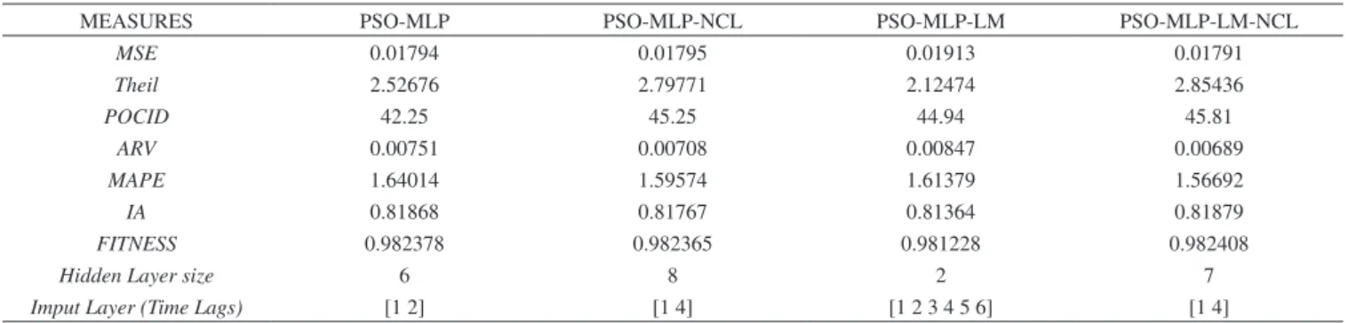
The most adequate model for the PM10 time-series forecasting was chosen after 10 experiments. Table 3 indicates that the PSO-MLP-LM-NCL model outperforms the other models in terms of MSE, POCID, ARV, MAPE, and IA. The selected model has two inputs (time lags 1 and 4) and a hidden layer with 7 processing units. Thus, the selected architecture was 2 – 7 – 1.
The ARV value for the PSO-MLP-LM-NCL model is smaller than 1. Therefore, the proposed model has a better performance than the time-series forecasting using the average of the series. In terms of IA, all models had similar results. Figure 5 shows the forecast made
by the PSO-MLP-LM-NCL model (dashed line) and the last 100 observed values (solid line).
Nitrogen dioxide series
The measurements conducted in the year 2002 for the NO2 series were used to assess the model validity. The NO2 series consists of 355 daily averages.
According to Table 4, the best suited model for the representation of the time series, chosen after 10 experiments, was PSO-MLP-NCL, which obtained the best results in terms of MSE and IA. Comparing to PSO-MLP-LM, the PSO-MLP-NCL model obtained a superior performance in terms of MSE, POCID, MAPE, and IA. The best model has three inputs (lags 1, 2, and 5) and 10 processing units in its hidden layer. Thus, the selected architecture was 3 – 10 – 1.
The selected model was capable of reaching a better performance than the time-series average (ARV less than 1). Figure 6 presents the observed data (solid line) and predicted data (dashed line) for the last 88 points of the series.
Table 1. Results for the CO series
MEASURES PSO-MLP PSO-MLP-NCL PSO-MLP-LM PSO-MLP-LM-NCL
MSE 0.00791 0.00686 0.00728 0.00884
Theil 1.51043 2.08514 0.92525 1.31084
POCID 55.61 58.19 54.23 52.24
ARV 0.00983 0.00929 0.00755 0.01038
MAPE 0.41014 0.39432 0.41446 0.43161
IA 0.76003 0.78052 0.77216 0.74616
FITNESS 0.99216 0.99319 0.99278 0.99124
Hidden Layer size 7 10 5 8
Imput Layer (Time Lags) [1 2] [1 6] [1 2 3 4] [3 7]
Figure 3. Result of the last 100 values of the prediction made by the
PSO--MLP-NCL model for the CO series (test set). Normalized observed and predicted values are presented
Table 2. Results for the SO2 series
MEASURES PSO-MLP PSO-MLP-NCL PSO-MLP-LM PSO-MLP-LM-NCL
MSE 0.00927 0.00913 0.00883 0.01046
Theil 2.62792 2.76644 2.57693 2.28375
POCID 48.54 47.95 47.91 46.97
ARV 0.01572 0.01498 0.01533 0.01241
MAPE 0.77784 0.75895 0.77051 0.8205
IA 0.7711 0.77286 0.77797 0.75025
FITNESS 0.990815 0.99095 0.991244 0.98965
Hidden Layer size 5 1 9 8
Imput Layer (Time Lags) [1 2] [1 5] [1 2 3] [1 4 6 8]
Figure 4. Result of the last 100 values of the prediction made by the
Table 3. Results for the PM10 series
MEASURES PSO-MLP PSO-MLP-NCL PSO-MLP-LM PSO-MLP-LM-NCL
MSE 0.01794 0.01795 0.01913 0.01791
Theil 2.52676 2.79771 2.12474 2.85436
POCID 42.25 45.25 44.94 45.81
ARV 0.00751 0.00708 0.00847 0.00689
MAPE 1.64014 1.59574 1.61379 1.56692
IA 0.81868 0.81767 0.81364 0.81879
FITNESS 0.982378 0.982365 0.981228 0.982408
Hidden Layer size 6 8 2 7
Imput Layer (Time Lags) [1 2] [1 4] [1 2 3 4 5 6] [1 4]
Table 4. Results for the NO2 series
MEASURES PSO-MLP PSO-MLP-NCL PSO-MLP-LM PSO-MLP-LM-NCL
MSE 0.2676 0.2551 0.02718 0.02605
Theil 1.74967 1.78871 0.77516 1.0454
POCID 45.55 44.44 41.57 44.44
ARV 0.02498 0.02587 0.01196 0.01605
MAPE 0.72517 0.70461 0.75287 0.62954
IA 0.76262 0.76856 0.75205 0.76189
FITNESS 0.97394 0.97512 0.97354 0.97462
Hidden Layer size 9 10 9 4
Imput Layer (Time Lags) [1 2] [1 2 5] [1 2] [3]
Figure 5. Result of the last 100 values of the prediction made by
PSO-MLP--LM-NCL model for the PM10 series (test set). Normalized observed and predicted values are presented
Figure 6. Result of the last 88 values of the prediction made by
PSO-MLP--NCL model for the NO2 series (test set). Normalized observed and predicted values are presented
CONCLUSIONS
In this study, a hybrid system for time-series forecasting of con-centration levels of air pollutants was evaluated. The system consists of an intelligent hybrid model composed of a PSO algorithm and an MLP ANN. PSO searches for a minimum number of time delays for proper time-series characterization and an optimized structure of a neural network in terms of input units, hidden processing units, initial weights, and biases of the ANN.
Four combined methods – MLP, MLP-NCL, PSO-MLP-LM, and PSO-MLP-LM-NCL – were applied to four series of natural phenomena (CO, SO2, PM10, and NO2).
The results were presented in terms of six measures: MSE, Theil, ARV, MAPE, POCID, and IA.
Among the proposed combinations, PSO-MLP-NCL found the best MLP configuration in two (CO and NO2) of the four time series addressed. For the time series of SO2 concentration, PSO-MLP-LM found the best model. Finally, PSO-MLP-LM-NCL found the best model for the time series of PM10.
The PSO-MLP-LM and PSO-MLP-LM-NCL models conjugate PSO with a gradient descent algorithm (LM) for MLP training. This hybridization combines exploitation and exploration characteristics. PSO provides exploratory behavior. However, one of the main diffi-culties with PSO is that once it finds a possible global minimum, its performance does not improve quickly enough (it stagnates), taking a long time to reach the best result in a particular search space area.25 Thus, when PSO is unable to substantially enhance network perfor-mance, the gradient descendent algorithm can exploit the search space locally, performing the search and achieving a local minimum within that specific area in less time.
Furthermore, the results obtained in this study are similar to those obtained from other approaches found in the literature. Brunelli ob-tained the best MSE of 0.02 for CO concentration in Boccadifalco,6 while the best result in the present study, in terms of MSE, was 0.007, obtained by the PSO-MLP-NCL model.
Athens, which are similar to the accuracy of the results obtained with the proposed method.17 Kukkonen et al. reported IA values between 0.42 and 0.77 in the prediction of PM10 in the Helsinki region.26 In the same study, Kukkonen et al.obtained IA values between 0.6 and 0.8 in NO2 prediction. The proposed methods in that study resulted in a mean IA value of 0.7 for NO2 prediction.26 Thus, the results obtained by the proposed method are in the same range with respect to other pollutant forecasting techniques that have been applied around the world.
The results show that the combination of PSO and MLP is a valid option for time-series forecasting of concentration levels of air pollutants, because it obtains a fair and accurate forecast at an acceptable computational cost. In particular, the results show that this approach may be an interesting tool to predict the concentration levels of pollutants in São Paulo, Brazil.
ACKNOWLEDGMENTS
We thank FACEPE and CNPq for the financial support to the research.
REFERENCES
1. Arbex, M. A.; de Souza Conceição, G. M.; Cendon, S.P.; Arbex, F.F.; Lopes, A.C.; Moysés, E.P.; Santiago, S.L.; Saldiva, P.H.; Pereira, L.A.; Braga, A.L.F.; J. of Epidemiology & Community Health 2009, 63, 777. 2. O’Neill, M.S; Bell, M.L; Ranjit, N.; Cifuentes, L.A.; Loomis, D.;
Gou-veia, N.; Borja-Aburto, V.H.; Epidemiology 2008, 19, 810.
3. Box, G. E. P.; Jenkins, G. M.; Time Series Analysis: Forecast and Con-trol, 3rd ed., Prentice Hall: New Jersey, 1994.
4. Khashei, M.; Bijari, M.; Appl. Soft Computing 2011, 11, 2664. 5. Haykin, S.; Neural Networks: A Comprehensive Foundation, 2nd ed.,
Prentice Hall: New Jersey, 1999.
6. Brunelli, U.; Atmos. Environ. 2007, 41, 2967.
7. Lu, W. Z.; Fan, H. Y.; Lo, S. M.; Neurocomputing 2003, 51, 387.
8. Eberhart, R.; Kennedy, J.; Proc. of Int. Conference on Neural Networks, Perth, Australia, 1995.
9. de M. Neto, P. S. G.; Petry, G. G.; Lima Junior, A. R.; Ferreira, T. A. E.; Proc. of Int. Joint Conference on Neural Networks, Atlanta, United States of America, 2009.
10. Zhao, L.; Yang, Y.; Expert Syst. with Appl. 2009, 36, 2805.
11. Feng, Y.; Zhang, W.; Sun, D.; Zhang, L.; Atmos. Environ. 2011, 45, 1979.
12. Valenzuela ,O.; Rojas, I.; Rojas, F.; Pomares, H.; Herrera, L.J.; Guillen, A.; Marquez, L.; Pasadas, M.; Fuzzy Sets and Syst. 2008, 159, 821. 13. Graves, D.; Pedrycz, W.; Neurocomputing 2009, 72, 1668. 14. Kumar, U.; Ridder, K. De; Atmos. Environ. 2010, 44, 4252.
15. Kurt,A.; Gulbagci, B.; Karaca, F.; Alagha, O.; Environ. Int. 2008, 34, 592.
16. Wang, D.; Lu, W. Z.; Ecol. Model. 2006, 198, 332. 17. Grivas, G.; Chaloulakou, A.; Atmos Environ. 2006, 40, 1216. 18. Dang, D.; Lu, W. Z.; Atmos. Environ. 2006, 40, 913.
19. de Mattos Neto, P. S. G.; Lima Junior, A. R.; Ferreira, T. A. E.; Proc. of Genetic and Evolutionary Computation Conference,Montréal, Canadá, 2009.
20. Shumway, R. H.; Stoffer, D. S.; Time series analysis and its applica-tions, 3rd ed., Springer: New York, 2011.
21. Takens, F.; Dynamical Systems and Turbulence 1980, 898, 366. 22. Coppin, B.; Artificial Intelligence Illuminated, 1st ed., Jones & Bartlett
Publishers: Sudbury, 2004.
23. CESTEB – SP, Companhia Ambiental do Estado de São Paulo; http:// www.cetesb.sp.gov.br. accessed in January 2012.
24. Prechelt, L.; Probenl: A set of neural network benchmark problems and benchmarking rules, Technical Report 21/94, 1994. http://citeseerx.ist. psu.edu/viewdoc/summary?doi=10.1.1.115.5355 accessed in January 2012
25. Noel, M. M.; Appl. Soft Computing. 2012, 12, 353.