CONTROLLER DESIGN TECHNIQUES FOR THE LOTKA–VOLTERRA
NONLINEAR SYSTEM
Magno Enrique Mendoza Meza
∗Amit Bhaya
∗Eugenius Kaszkurewicz
∗Dept. of Electrical Engineering, COPPE, Federal University of Rio de Janeiro, P.O. Box 68504, RJ 21945-970, BRAZIL
ABSTRACT
A large class of predator-prey models can be written as a non-linear dynamical system in one or two variables (species). In many contexts, it is necessary to introduce a control into these dynamics. In this paper we focus on models of two species, and assume, as is common in mathematical ecology, that the control corresponds to a proportional removal of the predator population. Six controller design techniques are ap-plied to the Lotka–Volterra model, which is thus used as a benchmark to evaluate and compare these techniques in an ecological context.
KEYWORDS: Adaptive control of oscillations, Control Lia-punov function, Immersion and Invariance, Induced internal feedback, Static sliding-mode control, Uncertain inputs.
RESUMO
Uma ampla classe de modelos do tipo predador-presa pode ser escrita como um sistema dinâmico não linear em uma ou duas variáveis (espécies). Em diversos contextos é ne-cessário introduzir um controle nessas dinâmicas. Este ar-tigo foca-se em modelos de duas variáveis. Assume-se, de acordo com a praxe em ecologia matemática, que o controle corresponde à remoção de uma proporção da população dos predadores (controle proporcional). Seis técnicas de projeto de controladores são aplicados ao modelo Lotka–Volterra, o qual é utilizado como um padrão ou “benchmark” para
ava-liar e comparar estas técnicas em um contexto ecológico.
PALAVRAS-CHAVE: Controle adaptativo de oscilações, Controle a modo deslizante estático, Entradas incertas, Fun-ção de Liapunov com controle, Imersão e invariância, Reali-mentação interna induzida.
1
INTRODUCTION
Physical, chemical and biological systems are inherently nonlinear (May, 1973; Slotine e Li, 1991; Khalil, 1992; Utkin, 1992). A large class of models that describe predator-prey population dynamics can be described as a nonlinear dynamic system. In this paper models of two species are considered and they have the following generic form
˙
x = f1(x) +f2(x)y (1) ˙
y = f3(x)y (2)
where the state variablexdenotes the prey density, the state variableydenotes the predator density, the functionsf1and
f3 describe the growth functions of the prey and predator
respectively andf2is a predator consumption function.
models, and has the following form
˙
x = r1x−a x y, ˙
y = −r2y+b x y,
(3)
where the parameterr1is the growth rate of the prey,r2is
the mortality rate of the predator,a,brepresent the interac-tion coefficients between the species; all parameters are pos-itives,f1 =r1x,f2 =−a x,f3 =−r2+b x. These
equa-tions constitute the simplest representation of the essence of the nonlinear predator-prey interaction (May, 1973; Gurney e Nisbet, 1998).
There have been many attempts to consider changing the Lotka–Volterra dynamics (3) by the introduction of controls and the main objective of this paper is to briefly present both techniques that have already been used, as well as some that have not and compare them with a new technique proposed in this paper.
We will briefly discuss the other techniques in section 3. Here we limit ourselves to a brief description of the proposed control.
Population dynamic models with threshold
control
The paper focuses on the introduction of an exogenous con-trol in models of populational dynamics of two species. The general model is as follows:
˙
x = f1(x) +f2(x)y, (4) ˙
y = f3(x)y−y u2, (5)
where the controlu2 corresponds to a proportional removal
of the predator population. We note that the dynamical sys-tem (4), (5) is in the so called regular form (Utkin, 1992), also called triangular or chained form. We can choosey = ˆyto control the subsystem (4) so thatxhas some desired behav-ior, and then designu2so thatyin (5) tracksyˆwhich is the
desired “input” for (4). However, in an ecological context, the controlling actionu2 must satisfy certain restrictions or
desirable characteristics that are discussed in the following section.
2
DESIRABLE
CHARACTERISTICS
OF
CONTROL IN AN ECOLOGICAL
CON-TEXT
Throughout this paper, the control term is to be understood as removal of a certain species.
In this context, the control must have the following charac-teristics:
• Implementation simplicity: (i) the mathematical
ex-pression of the control must be as simple as possible, (ii) the control must not depend on the system parame-ters so that they do not need to be estimated.
• Nonnegative control. This corresponds to the
propor-tional removal of one of the species. In other words, it is assumed that the control corresponds only to removal, i.e. we consider “harvesting” of a certain species.
• Minimal monitoring. Refers to the number of
popula-tion densities that need to be monitored to implement a certain control. In the context of the two species model (4), (5) if only one density is used to design feedback, we refer to this as output feedback; if both densities are used, then we call this state feedback.
• Promotion of coexistence. Both species must reach
sustainable equilibrium levels, in which the populations, in appropriate units, are both positive.
Finally, as far as units are concerned, note the following:
Density unit: The population density is the size of the
pop-ulation in relation to some space unit. Generally it is evaluated as the number of individuals or a population biomass, per unit area or volume.
Time unit: Time in ecological systems is usually measured
in days, weeks or years.
3
GENERAL APPROACHES FOR
CON-TROL OF NONLINEAR DYNAMIC
SYS-TEMS
In this section we briefly present six different techniques of nonlinear system design applied to the Lotka–Volterra (3) as a benchmark, with the objective of comparing them to the proposed control.
The set of general design methods of controllers for nonlin-ear systems can be divided in two subsets in the ecological context, as follows:
Techniques already applied to population dynam-ics:
• Fradkov e Pogromsky (1998) applied the so called speed gradient method of adaptive control of oscil-lations to control the popuoscil-lations of two competitive species. Their method was specific to the Lotka– Volterra model of population dynamics.
• Emel’yanov et al. (1998) presented a general method-ology, referred to as induced internal feedback, for the control of uncertain nonlinear dynamic systems. It is based on on-off control as well as continuous versions of the latter and applied to the Lotka–Volterra system.
• The proposed control is based on the application of con-trol Liapunov functions (Sontag, 1989), exploring the structure of the predator-prey systems and the backstep-ping idea (Sepulchre et al., 1997) for the regular form (Utkin, 1992), as well as using the concept of real and virtual equilibria (Costa et al., 2000) to derive an on-off or variable structure control.
Techniques not previously applied to population dynamics:
• Junger e Steil (2003) presented a new type of sliding motion which results from a special choice of the sliding surfaces. They define sliding surfaces such that these become explicitly dependent on the outputs of the dis-continuous block. Under this design, a special sliding mode characterizes the system dynamics, which they named static sliding mode, because it occurs along the static contour of the closed-loop systems.
• A new method to design asymptotically stabilizing and adaptive control laws for nonlinear systems is presented in Astolfi e Ortega (2003). The method relies upon the notions of system immersion and manifold invariance and, in principle, does not require the knowledge of a (control) Lyapunov function.
3.1
Design of the controller according to
Emel’yanov et al.
The following theorem from Emel’yanov et al. (1998) is pre-sented.
Theorem 1 Consider the system
˙
x=ϕ1(x, y) ˙
y=ϕ2(x, y) +B(t)u
(6)
z= [x y]T,B=diag(b1, . . . , bn),bi(·)∈
1
L, L
,ϕ1,ϕ2
are continuous, Lipschitz locally and unknown.
There is a continuous controlusuch that the trajectories of
the system (6) approach the setGand enter in it in finite time,
where
G:={z:s ≤σ(x, t)}
with
s:=y−v(x, t),
in closed loop,v(x, t)is the trajectory to be tracked,σ(x, t)
is a tracking error tolerance. The control has the following form:
u=− s
sΨ (s, σ)F(z, t).
Emel’yanov et al. procedure applied to the
Lotka–Volterra model with control only in
the predator
Consider system (3) with control applied only to the preda-tor:
˙
x=r1x−a x y, ˙
y=−r2y+b x y−u.
Procedure:
1. Choose the equilibrium point, at which is desired to sta-bilize the system, for a prey densityM. It must satisfy
M >supr2
b
,
and the predator density must satisfy
yeq =r1
a.
2. Suppose that it is necessary to maintainxclose toM, i.e.,|x−M|< δ. Introduce the constantsL1,L2andσ
(σas an induced error tolerance, in this case a constant). The constants must satisfy
L1+σ <
r1
a, L2−σ > r1
a.
3. Choose the internal feedback operatorv(x), e.g. see Figure 1,
v(x) =L1+(L2−L1) max
0,min
1,x−M +δ
2δ
.
4. The “induced error vector” is defined as:
s:=y−v(x).
5. The induced error toleranceσ(x, t)is chosen such that:
½ ¾
½
¾ ¼
Æ Æ ´µ
Figure 1:Induced internal feedback operator.
6. Check the conditions
dy dx >
dv dx ,
to guarantee the invariance of regionG:={z :s ≤ σ}.
7. Analyze the behavior of the system in the following re-gions:
|x−M|> δ, |x−M|< δ.
From the analysis, we obtain the gainF.
8. The control law is:
u=F x ymax
0,min
1,s−σ
2σ
.
In this case the following restriction (see Emel’yanov et al. (1998) for details) must be satisfied:
xeq−σ >supr2
b .
For comparison, we use the parameters in Costa et al. (2000), substituting the values of these parameters in the constraints, the following numerical relations are obtained:
xeq >1.2, F > b+L2−L1
2δ a= 1.625.
Under these constraints, feasible values of desired equilib-rium point as well as of the control effort are chosen
xeq = 1.25, yeq= 1, L
1= 0.75, L2= 1.25,
F = 1.625, M = 1.25, δ=σ= 0.2.
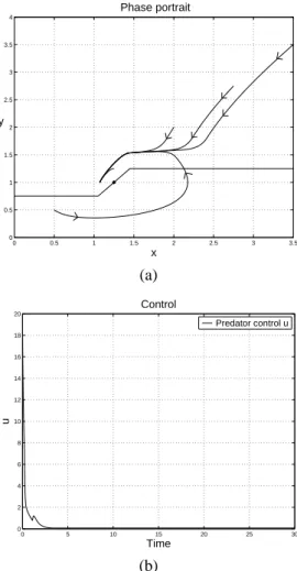
The chosen value of xeq is the same used in Costa et al. (2000). The control is given by:
u = F x ymax
0,min
1,s−σ
2σ
0 0.5 1 1.5 2 2.5 3 3.5
0 0.5 1 1.5 2 2.5 3 3.5 4
x y
Phase portrait
(a)
0 5 10 15 20 25 30
0 2 4 6 8 10 12 14 16 18 20
Time
u
Control
Predator control u
(b)
Figure 2: (a) Phase plane of Lotka–Volterra model subject to Emel’yanov’s control. (b) Time evolution of the control actionu. Para-meter valuesr1 = 1,r2 = 1,a= 1,b = 1,F = 1.625,δ= 0.2and σ= 0.2.
3.2
Proposed Control design
The idea of backstepping will be explained in a simple form for equations (7), (8). The state variableyis taken as a
fic-titious input (ficfic-titious control), denoted asu1, to the prey
subsystem (7). A control Liapunov function (CLF) is used to design the controlu1such that the prey subsystem stabilizes
in the desired equilibrium (for the prey). The next step is to design the (real control)u2, involving removal of predators,
such that the state of predator subsystemytracks the design inputu1. Again, the design is made using another CLF. In
The resulting control system is described by:
˙
x = f1(x) +f2(x)y (7) ˙
y = f3(x)y−y u2 (8)
in whichu2is the control (=threshold policy) to be designed.
In other words, choose:
u2=ε2φ(τ, σ), (9)
withε2a control effort parameter to be designed andφ(τ, σ)
defined as,
φ(τ, σ) =
1 if τ >0
0 if τ <0, (10)
whereτ is a variable that defines the threshold, which is de-pendent on the system states.
The design of the CLF proceeds as follows: In the first sub-system (7), lety=u1be a fictitious control. Choose a CLF
as
V1(x) = 1
2(x−xd) 2
(11)
wherexdis the desired equilibrium for the first subsystem. Note that a coordinate change can be made such that the de-sired valuexdoccurs at the origin.
Calculating the derivative ofV1 along the trajectories of (7)
gives:
˙
V1= (x−xd) (f1(x) +f2(x)u1). (12)
Now, assume for simplicity thatu1is proportional to the prey
densityx, i.e.,
u1=ε x. (13)
Then the parameterεmust be chosen such thatV˙1<0.
Now,u2must be chosen such thatu1satisfies (13).
There-fore, choose the thresholdτas follows
τ=y−u1=y−ε x, (14)
and a CLFV2as
V2= 1 2τ
2
, (15)
with the objective of maintainingτ = 0and thus satisfying (13).
The derivativeV2along the trajectories of (7), (8) leads to ˙
V2=τ[−ε 1]
f1(x) +f2(x)y
f3(x)y−y u2 .
(16)
Now the specific properties of functionsf1, f2 andf3 are
used to chooseεandε2such that both functions satisfyV˙1< 0andV˙2<0, proving stability. The details of the choice and
stability proofs can be found in Meza (2004) and have not been included in this paper for lack of space.
Simulation of the behavior of the Lotka–
Volterra model subject to the horizontal
threshold policy applied only to the
preda-tor
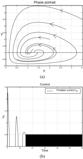
The Lotka–Volterra subject to the threshold policy applied only to the predator stabilizes the system around the thresh-old as shown in the phase plane in Figure 3.a. Time evolution of the control is shown in Figure 3.b. The sliding equilib-rium is (xeqsl, y
eq
sl) = (1.25,1). In this caseτ is chosen as τ =y−ysleq.
0 0.5 1 1.5 2 2.5 3 3.5
0 0.5 1 1.5 2 2.5 3 3.5 4 4.5
x y
Phase portrait
(a)
0 10 20 30 40 50 60
0 0.5 1 1.5 2 2.5
Time
u2
Control
Predator control u2
(b)
Figure 3: (a) Phase plane of the Lotka–Volterra model subject to the threshold policy. (b) Time evolution of the controlling action. Parameter valuesr1= 1,r2= 1,a= 1,b= 1eε2= 0.5
3.3
Design of the controller according to
Fradkov et al.
birth rate of the prey. In this case model (3) is modified as follows:
˙
x = r1x−a x y ˙
y = −r2y+b x y+y u
(17)
whereuis the controlling action.
It is not difficult to show that the uncontrolled system (u≡0) has an infinite number of periodic solutions, provided that x(0) > 0,y(0) > 0, which correspond to the existence of the following first integral:
W(x, y) =
b x−r2−r2log
b x
r2
+
a y−r1−r1 log
a y
r1
. (18)
Indeed,
˙
W(x, y) = 0
along any solution of (3) (x(0)>0,y(0)>0), which means that the quantityW preserves its constant value. The first integral (18) can be interpreted as a “total energy” of the “predator-prey” system and the control goal can be stated in terms of achieving the desired level of quantityW
W(x(t), y(t))→W∗ as t→ ∞. (19)
whereW∗is the desired level of the first intergral.
A control goal of this kind can be achieved by the speed gradient (SG) method, see Fradkov e Pogromsky (1998, Chap. 2). Introduce the following objective function Q :
R×R→R+:
Q(x, y) =1
2(W(x, y)−W∗) 2
.
Then its time derivative with respect to the system (17) gives
˙
Q(x, y) = (W(x, y)−W∗) (a y u−r2u).
Calculating the gradient inugives:
∂Q˙
∂u(x, y) = (W(x, y)−W∗) (a y−r2).
According to Theorem 2.21 in Fradkov e Pogromsky (1998, pag. 101) the following SG algorithm
u(t) =−γ(W(x(t), y(t))−W∗) (a y(t)−r2) (20)
achieves the goal (19) forγ >0and almost all initial condi-tions satisfyingx(t)>0,y(t)>0.
To illustrate the theoretical results we carried out computer simulation of the model (17). The SG algorithm (20) for the system (17) with the following parameter valuesr1= 1,
r2= 1,a= 1,b= 1is as follows
W(x, y) = (x−1−log(x)) + (y−1−log(y))
andu(t)is
u(t) =−γ(W(x(t), y(t))−W∗) (y(t)−1).
Simulation of the behavior of the Lotka–
Volterra model subject to the control
ac-cording to Fradkov et al.
0 0.5 1 1.5 2 2.5 3 3.5
0 0.5 1 1.5 2 2.5 3 3.5
x y
Phase portrait
(a)
0 5 10 15 20 25 30
−10 0 10 20 30 40 50
Time
u2
Control
Predator control u2
(b)
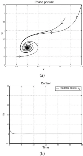
Figure 4: (a) Phase plane of the Lotka–Volterra model subject to a SG algorithm. (b) Time evolution of the controlling actionu. Parameter values r1= 1,r2= 1,a= 1,b= 1,γ= 2andW∗=−0.1.
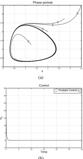
It is seen that choosing different values of the desired “en-ergy” levelW∗we can achieve significantly different
behav-ior of the controlled system, as shown in Figures 4 and 5 (Fradkov e Pogromsky, 1998). In the case where W∗ =
−0.1, the system approaches asymptotically to the equilib-rium point(r1/a , r2/b)as can be observed in Figure 4 and
in the case whereW∗= 0.5the system displays a limit cycle
as can be observed in Figure 5.
3.4
Control of systems in the presence of
uncertain inputs
Consider the Lotka–Volterra model under the effect of a har-vesting strategy with constant efforts in both species, h1x
0 0.5 1 1.5 2 2.5 3 3.5 0
0.5 1 1.5 2 2.5 3 3.5
x y
Phase portrait
(a)
0 5 10 15 20 25 30
−5 0 5 10 15 20 25 30 35
Time
u2
Control
Predator control u2
(b)
Figure 5: (a) Phase plane of the Lotka–Volterra model subject to a SG algorithm. (b) Time evolution of the controlling actionu. Parameter values r1= 1,r2= 1,a= 1,b= 1,γ= 2andW∗= 0.5.
added, as well as additional controlsp1andp2, as follows: ˙
x=r1x−a x y−x s1+p1−h1x, ˙
y=−r2y+b x y−y s2+p2−h2y.
(21)
The uncertainty is such that|s1| ≤sm1and|s2| ≤sm2. The
corresponding equilibrium point is(x∗
, y∗
). The problem is to maintain this equilibrium point under the uncertaintiess1
ands2using the controlsp1andp2.
According to the method in Vincent et al. (1985), the idea is to use knowledge of the reachable setRto calculate the extreme effects of the uncertainty over this set and then use this information in feedback controller design.
A Liapunov function for (21) withs1 =s2=p1 =p2 = 0,
also based on the first integral, is given as follows
V(x, y) =x−x∗
−x∗ lnx
x∗
+y−y∗
−y∗ ln
y y∗
(22)
which is valid throughout the regionXdefined by
X =
x∈R2|x >0, y >0
. (23)
The region R depends on the specific parameters used and the equilibrium points of (21) withp1=p2= 0,s1=±sm1,
s2 =±sm2 andsm1 = 0.2,sm2 = 0.15,h1 = 0.25,h2 = 0.25. Therefore,x∗
= 1.25,y∗
= 0.75,ρ1 = 1.45×0.2,
ρ2 = 0.95×0.15and d = 0.25, we obtain sm1 = 0.2,
sm2 = 0.15,h1 = 0.25,h2 = 0.25. Therefore,x∗ = 1.25,
y∗= 0.75,ρ
1= 1.45×0.2,ρ2= 0.95×0.15andd= 0.25,
we obtain
∂V ∂x = 1−
x∗
x e1 ∂V
∂y = 1− y∗
y e2
(24)
Letω=
(x−x∗)2+ (y−y∗)2, then the control laws
be-come
p1=
−ρ1sign(e1) if |e1|> ζ
−ρ1e1/ζ if |e1| ≤ζ
−ρ1 exp[−l1(ω−d)]sign(e1) if ω > d
(25)
p2=
−ρ2sign(e2) if |e2|> ζ
−ρ2e2/ζ if |e2| ≤ζ
−ρ2 exp[−l2(ω−d)]sign(e2) if ω > d
(26)
Simulation of the behavior of the Lotka–
Volterra model subject to the control
ac-cording to Vincent et al.
Consider the following parameter values: r1 = r2 = a =
b = 1,x∗ = 1.25,y∗ = 0.75,ζ = 0.01,l
1 = 1,l2 = 1,
s1(t) = 0.2 cos(t),s2(t) = 0.15 cos(t).
Figure 6.a shows the simulation of model (21) under pertur-bations of types1(t) =−0.20 cos(t),s2(t) =−0.15 cos(t)
and subject to the control of type (25), (26). Figure 6.b shows the time evolution of the control action.
3.5
Static sliding-mode control
Consider a nonlinear unstable plant
˙
z=a(z) +B(z)ξ, z(0)=0. (27)
The goal is to define a controlξsuch thatz(t)→0fort→
∞. This is achieved by defining a suitable switching surface
σ=r(z)−D(z)sign(σ) (28)
wherer(z),D(z)must be chosen. The following theorem
0 0.5 1 1.5 2 2.5 3 3.5 0
0.5 1 1.5 2 2.5 3 3.5 4 4.5 5
x y
Phase portrait
(a)
0 5 10 15 20 25 30
−0.2 0 0.2 0.4 0.6 0.8 1 1.2 1.4
Time
u1 ,u2
Controls
Prey control u1
Predator control u2
(b)
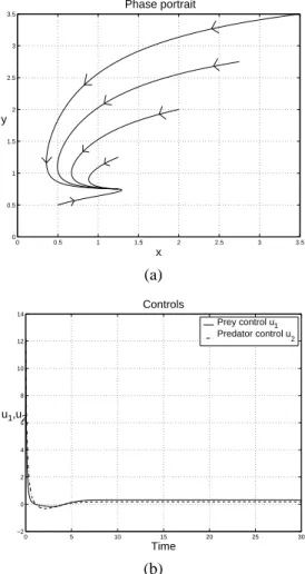
Figure 6:(a) Phase plane of the Lotka–Volterra model subject to the con-trol according to Vincent. (b) Time evolution of the concon-trolling actionsu1, u2.
Junger e Steil (2003) show how the static sliding-mode ap-proach can be effectively applied for nonlinear plant control. They show that the functionsr(z)andD(z), which were
as-sumed to be given previously, can effectively be constructed for an interesting and large class of nonlinear systems. They defined the sliding-mode control as follows.
Definition 3.1 (Sliding-Mode Control. Definition VI.1 in
Junger e Steil (2003)): Ifξ(t) guaranteesσ(t) ≡ 0, ∀t ∈
[t1, t2], then it is called sliding-mode control.
Theorem 2 (Theorem VI.1 in Junger e Steil (2003)) Let
v(z)be an r-dimensional continuous vector-function such
that z(t) → 0, whenever v(z) → 0. Assume that
det [Jv(z)B(z)] = 0 for allz = 0, whereJv(z)is the
Ja-cobian matrix ofv(z), then there exists a stabilizing static
sliding-mode control.
Constructive procedure for control design
(and proof of Theorem 2)
With regard to the plant (27) the derivative ofv(z)is
˙
v=Jv(z) [a(z) +B(z)ξ]. (29)
Define the system of differential equations
˙
v=−K v (30)
whereK = diag{ki} > 0 is an arbitraryr×rconstant
positive diagonal matrix.
Substitution from (29) yields
Jv(z) (a(z) +B(z)ξ) =−Kv(z). (31)
The sliding surface is defined by following relation:
σ=Jv(z) (a(z) +B(z)ξ) +Kv(z). (32)
Then, r(z, t) = Jv(z)a(z) + Kv(z), D(z, t) =
−Jv(z)B(z)andσ≡0by construction. Now, the system is
in sliding mode whenever the static sliding-mode control
ξ=−(Jv(z)B(z))−1(Jv(z)a(z) +Kv(z)) (33)
is applied. Under (33), equality (30) holds. Therefore,
v(z)→0and, hencez(t)→0.
Junger et al.
procedure applied to the
Lotka–Volterra model
Consider a nonlinear system of type Lotka–Volterra that we desire to stabilize with the help of the static sliding-mode approach. Assume that the plant (27) has the following para-meters:
a(z) =
r1x−a x y
−r2y+b x y
,B(z) =
−x −y
. (34)
Remark 3.1 Note that the static sliding-mode control is
ap-plied to both species.
Chose the functionv(z)as[x−xth y−yth]. The Jacobian Jv(z)B(z) = [−x −y]is nonzero for allz= 0.
The corresponding stabilizing static sliding mode continuous control has the form
ξ= r1x−a x y−r2y+b x y+k(x−xth) +k(y−yth)
x+y .
(35) The Lotka–Volterra system under the static sliding mode control is as follows
˙
x=r1x−a x y−x ξ, ˙
y=−r2y+b x y−y ξ.
Simulation of the behavior of the Lotka–
Volterra model subject to the control
ac-cording to Junger et al.
Figure 7 shows the dynamics of the Lotka–Volterra system subject to the static sliding mode control.
0 0.5 1 1.5 2 2.5 3 3.5
0 0.5 1 1.5 2 2.5 3 3.5
x y
Phase portrait
(a)
0 5 10 15 20 25 30
−2 0 2 4 6 8 10 12 14
Time u1,u2
Controls
Prey control u1
Predator control u
2
(b)
Figure 7:(a) Phase plane of the Lotka–Volterra model subject to the sta-tic sliding mode continuous control. (b) Time evolution of the controlling actions. Parameter valuesr1 = 1,r2 = 1,a= 1,b = 1,k = 1.25, xth= 1.25andyth= 0.75.
3.6
Immersion and Invariance for
Stabi-lization of Nonlinear Systems
Consider the Lotka–Volterra system with a control of type Immersion and Invariance (I & I) applied only to the predator as follows
˙
x = r1x−a x y ˙
y = −r2y+b x y+u2
(37)
with z = [x y]T, u
2 ∈ R, n = 2,p = m = 1and the
following mappings are defined:
α(·) : R→R π(·) :R→R2 c(·) :R→R φ(·) : R2→
R ψ(·,·) :R2×1→
R
such that the following hold.
H1) (Target system) Choose the system
˙
ξ=−ξ+xth (38)
withξ ∈ Rand such that it has a globally asymptoti-cally stable equilibrium atξ∗=xthand
x∗
= π1(ξ ∗
) =xth y∗
= π2(ξ ∗
)
then
x=π1(ξ) = 2ξ−xth
from the first equation of (37) we obtain
2(−ξ+xth) =r1(2ξ−xth)−a(2ξ−xth)π2
then
π2=
r1(2ξ−xth) + 2ξ−2xth
a(2ξ−xth) .
H2) (Immersion condition) The functionc(ξ)is defined im-plicitly as:
−r2π2+b(2ξ−xth)π2+c(ξ) =
∂π2
∂ξ (2ξ−xth).
H3) (Implicit manifold) The manifoldz=π(ξ)can be de-scribed by
φ(x, y) =y−r1x+x−xth a x
H4) (Manifold attractivity and trajectory boundedness) The
dynamics on the manifold is calculated as
˙
v= ∂φ
∂z[f(z) +g(z)ψ(z, v)]
then
˙
v=−xth a x2 1
r1x−a x y −r2y+b x y+ψ(z, v)
˙
v=−xth
a x2(r1x−a x y)−r2y+b x y+ψ(z, v).
The design I & I is completed by choosing
ψ(z, v) = xth
which produces the closed loop dynamics
˙
x = r1x−a x y ˙
y = xth
a x2(r1x−a x y)−v ˙
v = −v.
(39)
Hence, to complete the design it only remains to show that all trajectories of (39) are bounded. Consider the coordinate transformation
η=y−r1x+x−xth a x
yielding
˙
x = −(a η+ 1)x+xth
˙
η = −v
˙
v = −v.
(40)
Note thatx(t),η(t)andv(t)are bounded for alltand the control law is obtained as
u2=ψ(z, v)−η =
xth
a x2(r1x−a x y) +r2y
−b x y−y+r1x+x−xth
a x .
Simulation of the behavior of the Lotka–
Volterra model subject to the control
ac-cording to Astolfi et al.
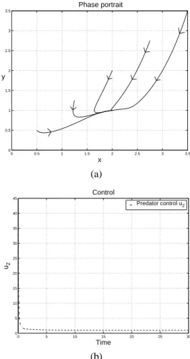
Figure 8 show the dynamics of the Lotka–Volterra system under the control law I & I.
4
COMPARISON
OF
THE
DIFFERENT
CONTROL TECHNIQUES
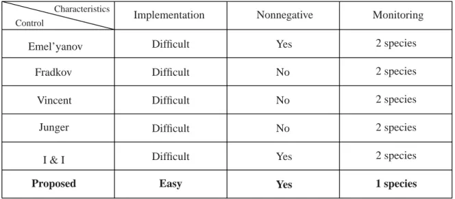
We use the terminology established in section 2 to make a comparison of the different techniques in a tabular form:
Table 1 shows that only the proposed control possesses all the desirable charateristics specified in Section 2. To be com-pletely fair, it should be pointed out that we have not explic-itly compared control with respect to robustness, although it is well known (Utkin, 1992) that all variable structure de-signs, such as the one proposed in this paper, have an inherent robustness to bounded uncertainty. On the other hand, given the considerably greater difficulty, or even impossibility, in the implementation of the other controls, it seems reasonable to limit our comparison to the items in the columns of Table 1.
5
CONCLUDING REMARKS
The proposed control possess all the desirable characteristics of a control to be applied in an ecological context, i.e. (i)
0 0.5 1 1.5 2 2.5 3 3.5
0 0.5 1 1.5 2 2.5 3 3.5
x y
Phase portrait
(a)
0 5 10 15 20 25 30
0 5 10 15 20 25 30 35 40 45
Time
u2
Control
Predator control u2
(b)
Figure 8:(a) Phase plane of the Lotka–Volterra model subject to the con-trol I & I. (b) Time evolution of the concon-trolling action. Parameter values r1= 1,r2= 1,a= 1,b= 1,k= 1andxth= 2.
easy to implement, i.e., it is a proportional control; (ii) the control is carried through the removal of only one species; (iii) only one species needs to be monitored; and (iv) species coexistence is achieved. Moreover, in comparison with sev-eral existing methods, both old and new, it seems to be the only one that combines all these desirable characteristics.
In terms of future work along the lines initiated in this paper, we mention a few topics.
Table 1: Comparison of control techniques for the Lotka–Volterra system
Characteristics
Control
Implementation
Nonnegative
Monitoring
Emel’yanov
Fradkov
Vincent
Junger
I & I
Proposed
Difficult
Difficult
Difficult
Difficult
Difficult
Easy
Yes
Yes
Yes
No
No
No
2 species
2 species
2 species
2 species
2 species
1 species
Some pointers to technical results that may be useful in this context are Tarbouriech et al. (2000), Mazenc e Niculescu (2001), Dercole et al. (2003).
Models of virus dynamics (Nowak e May, 2000) are very similar to the predator-prey models studied in this paper. There is great current interest in systematically finding “pro-tocols"(controls) that are capable of stabilizing virus popula-tions at low levels (Wein et al., 1997) and, once again, desir-able methods must have most of the characteristics stipulated in Section 2. We expect that the control design proposed in this paper will be applicable to this class of problems as well.
Finally, there has been recent interest in applying bifurca-tion analysis to planar populabifurca-tion dynamics models, and pre-liminary work of this kind can be found in Kuznetsov et al. (2003), Cunha et al. (2003), Moreno et al. (2003).
ACKNOWLEDGMENT
This research was partially financed by Project
Nos. 140811/2002-8, 551863/2002-1, 471262/03-0 of CNPq, No. E-26/150.505/2002, E-26/152.177/2003 of FAPERJ and also by the agency CAPES. Corresponding authors: Magno E. Mendoza Meza, Amit Bhaya.
REFERENCES
Astolfi, A. e Ortega, R. (2003). Immersion and invari-ance: A new tool for stabilization and adaptive con-trol of nonlinear systems, IEEE Trans. Automat.
Con-trol 46(4): 590–606.
Beddington, J. R. e May, R. M. (1977). Harvesting natural populations in a randomly fluctuating environment,
Sci-ence 197: 463–465.
Costa, M. I. S., Kaszkurewicz, E., Bhaya, A. e Hsu, L. (2000). Achieving global convergence to an equilib-rium population in predator-prey systems by the use of discontinuous harvesting policy, Ecological Modelling
128: 89–99.
Cunha, F. B., Pagano, D. J. e Moreno, U. F. (2003). Slid-ing bifurcations of equilibria in planar variable struc-ture systems, IEEE Trans. Circuits and Systems–I:
Fun-damental Theory and Applications 50(8): 1129–1134.
Dercole, F., Gragnani, A., Kuznetsov, Y. A. e Rinaldi, S. (2003). Numerical sliding bifurcation analysis: An ap-plication to a relay control system, IEEE Trans. Circuits
and Systems–I: Fundamental Theory and Applications
50(8): 1058–1063.
Emel’yanov, S. V., Burovoi, I. A. e Levada, F. Y. (1998).
Control of Indefinite Nonlinear Dynamics Systems, Vol.
231 of Lecture Notes in Control and Information
Sci-ences, Springer - Verlag, Great Britain.
Fradkov, A. L. e Pogromsky, A. Y. (1998). Introduction to
Control of Oscillations and Chaos, Vol. 35 of Nonlin-ear Science, World Scientific, Singapore.
Gurney, W. S. C. e Nisbet, R. M. (1998). Ecological
Junger, I. B. e Steil, J. J. (2003). Static sliding-motion phe-nomena in dynamical systems, IEEE Trans. Automat.
Control 48(4): 680–686.
Khalil, H. K. (1992). Nonlinear Systems, Macmillan Pub-lishing.
Kuang, Y. (1993). Delay Differential Equations with
Appli-cations in Population Dynamics, Academic Press, San
Diego.
Kuznetsov, Y. A., Rinaldi, S. e Gragnani, A. (2003). One-parameter bifurcations in planar Filippov sys-tems, International Journal of Bifurcation and Chaos
13(8): 2157–2188.
Lee, C. S. e Leitmann, G. (1983). On optimal long-term management of some ecological systems subject to uncertain disturbances, Internat. J. Systems Science
14(8): 979–994.
May, R. (1973). Stability and Complexity in Model
Ecosys-tems, Princeton University Press.
Mazenc, F. e Niculescu, S.-I. (2001). Lyapunov stability analysis for nonlinear delay systems, Systems and
Con-trol Letters 42(4): 245–251.
Meza, M. E. M. (2004). Nonlinear systems
of the predator-prey type: Control design
using Liapunov Functions. Available at
http://www.nacad.ufrj.br/˜amit/teses_dsc_or/ tese_dsc_meza2004.pdf.
Moreno, U. F., Peres, P. L. D. e Bonatti, I. S. (2003). Analy-sis of piecewise-linear oscillators with hystereAnaly-sis, IEEE
Trans. Circuits and Systems–I: Fundamental Theory and Applications 50(8): 1120–1124.
Nowak, M. A. e May, R. M. (2000). Virus dynamics:
Mathe-matical principles of immunology and virology, Oxford
University Press, Oxford.
Sepulchre, R., Jankovi´c, M. e Kokotovi´c, P. (1997).
Con-structive Nonlinear Control, Series on
Communi-cations and Control Engineering (CCES), Springer-Verlag, London.
Slotine, J.-J. E. e Li, W. (1991). Applied Nonlinear Control, Prentice Hall, Englewood Cliffs, New Jersey.
Sontag, E. D. (1989). A ‘universal’ construction of Artstein’s theorem on nonlinear stabilization, Systems and
Con-trol Letters 13: 117–123.
Steele, J. H. e Henderson, E. W. (1984). Modeling long-term in fish stocks, Science 224: 985–987.
Tarbouriech, S., Peres, P. L. D., Garcia, G. e Queinnec, I. (2000). Delay-dependent stabilization of time-delay systems with saturating actuators, Proceeding of the
39thIEEE Conference on Decision and Control,
Syd-ney, Australia, pp. 3248–3253.
Utkin, V. I. (1992). Sliding Modes In Control And
Optimiza-tion, Springer-Verlag, Berlin.
Vincent, T. L., Lee, C. S. e Goh, B. S. (1985). Maintenance of an equilibrium state in the presence of uncertain inputs,
Internat. J. Systems Science 16(11): 1335–1344.