THE LINEAR INTERPOLATION METHOD: A SAMPLING THEOREM
APPROACH
Pedro L. D. Peres
∗Ivanil S. Bonatti
∗Walter C. Borelli
∗∗
Faculdade de Engenharia El´etrica e de Computa¸c˜ao, Universidade Estadual de Campinas, CP 6101 13081-970, Campinas - SP - Brasil.
RESUMO
Uma aula sobre o teorema da amostragem como um m´etodo de interpola¸c˜ao ´e apresentada neste trabalho. A rela¸c˜ao entre a interpola¸c˜ao linear e o teorema da amostragem ´e real¸cada pelo uso de pulsos triangula-res aproximando fun¸c˜oes sampling. Al´em disso, ´e feita uma compara¸c˜ao entre a interpola¸c˜ao linear e a s´erie em uma base n˜ao ortogonal composta de pulsos triangulares igualmente espa¸cados. A interpola¸c˜ao usa os valores das amostras da fun¸c˜ao e os coeficientes da s´erie s˜ao obtidos minimizando o erro quadr´atico entre a fun¸c˜ao original e a s´erie.
PALAVRAS-CHAVE: Teorema da amostragem, interpola-¸c˜ao, s´erie de Fourier, bases n˜ao-ortonormais.
ABSTRACT
A lecture note introducing the sampling theorem as an interpolation method is presented. The relationship be-tween piecewise linear approximation and the sampling theorem is highlighted by the use of triangular pulses in-stead of sampling functions. Furthermore, a comparison of the linear interpolation with a series on a nonorthog-onal basis composed of equally spaced triangular pulses is provided. The interpolation uses the sample values of
Artigo submetido em 24/05/2001
1a. Revis˜ao em 8/10/2002; 2a. Revis˜ao 21/10/2002
Aceito sob recomenda¸c˜ao do Ed. Assoc. Prof. Jos´e R. C. Piqueira
the function whereas the series coefficients are obtained by minimizing the quadratic error between the original function and the series.
KEYWORDS: Sampling theorem, interpolation, Fourier series, nonorthonormal basis.
1
INTRODUCTION
The sampling theorem is usually interpreted as the re-sult of an ideal filtering applied to a sequence of impulses modulated by the original signal values at specific in-stants of time (Burrus et al., 1998), (Carlson, 1975), (Chen, 1989), (Chui, 1997), (Kwakernaak and Sivan, 1991), (Oppenheim et al., 1983), (Lathi, 1965), (Rabiner and Schafer, 1978), (Sinha, 1991), (Therrien, 1992).
As an alternative way to introduce the sampling the-orem, consider the following classroom problem: a se-quence of equally spaced points of an unknown function is given in a Cartesian plot and the students are re-quired to draw the best approximation to the function. Since the function is not known, this problem has not a closed solution but a good result could be obtained if the interpolation via the sampling theorem was used (see equation (14)).
To overcome the difficulties of drawing the sampling function (defined as Sa(t)sin(t)/t), the students are
figure 1. Following this strategy, the students can easily solve the problem by summing weighted equally spaced triangles (the result can be seen in figure 2). Surprised by this result, the students realized that this procedure is equivalent to simply joining adjacent points by line-segments.
Motivated by this classroom experiment, this paper is devoted to analyze the interpolation aspects of the sam-pling theorem in the context of Fourier series. In this sense, an alternative proof of the sampling theorem is provided, resulting from the projection of the signal on an orthogonal basis of sampling functions. It is impor-tant to emphasize that this proof is not usual in under-graduate textbooks, which in general prefer an interpre-tation coming from ideal filtering.
The paper is organized as follows: at first, the concept of orthogonal functions is presented and the proof of the sampling theorem is given. Next, using a triangu-lar pulse as a convenient approximation of the sampling function, it is shown that the signal recovering is in fact the same as a linear interpolation. Furthermore, the co-efficients of the actual orthogonal projection on a basis formed up by these triangular pulses are evaluated, in order to distinguish them from the sample values of the function (both approximations are linear, but only the former one minimizes the quadratic error).
2
PRELIMINARIES
An important problem in signal theory concerns the re-construction of a signal from a given set of parameters, as for instance, the Fourier series coefficients or the sam-ples of the signal equally spaced in time.
In order to construct a good series approximation for a class of signals, some error criterion must be assumed. Any positive decreasing monotonic function could be used, but an interesting one is the quadratic error mea-surement, which provides the orthogonal projection as the solution of a set of linear equations, as shown:
Consider {gk(t), k ∈ Z} an infinite dimensional set of
real orthogonal signals, i.e.
gk(t)gl(t)= 0 , k=l k, l∈Z (1)
gk2(t)
>0 (2)
whereZ{0,±1,±2, . . .} and
gk(t)gl(t)
+∞
−∞
gk(t)gl(t)dt (3)
The problem of reconstructing a given real signal f(t)
can be formulated as
min
ck
ǫ2(t)
(4)
where
ǫ(t)f(t)−
∞
k=−∞
ckgk(t) (5)
Note that ǫ2(t)
is a quadratic function with respect to
ck, thus a strictly convex function with a global
mini-mum. The optimal solution is then
ck =
f(t)gk(t)
g2
k(t)
, k∈Z (6)
Observe thatǫ(t) is orthogonal to allgk(t) elements of
the basis.
3
INTERPOLATION METHOD
Consider the set of orthogonal (with normT) sampling functions
gk(t)Sa
π
T(t−kT)
, k∈Z (7)
The projection of a signalf(t) on this set of functions can be done by determining the coefficientsck, that is
f(t) =
+∞
k=−∞
ckgk(t) (8)
with
ck =
1
T +∞
−∞
f(t)gk(t)dt (9)
Since the integral of a function (from−∞to∞) can be computed as its Fourier transform atω= 0, one gets
ck =
1
T F
f(t)Sa
π
T(t−kT)
ω= 0
= 1
T
1
2π F[f(t)]∗ F
Sa
π
T(t−kT)
ω= 0
= 1
2π F(ω)∗[G(ω) exp(−jωkT)] ω= 0 (10) whereF[·] is the Fourier transform of [·],G(ω) is given by
G(ω) =
0 for |ω|> π/T
1 for |ω|< π/T
(11)
and∗denotes the convolution operator.
Then
ck =
1 2π
+π/T
−π/T
If f(t) is band-limited, i.e. F(ω) = 0 for | ω |> 2πB,
B being the maximum frequency of the signalf(t), and also ifT <1/2B, i.e. the sampling rate is greater than the double of the maximum frequency off(t),ckis given
by
ck =
1 2π
+∞
−∞
F(ω) exp(jωkT)dω=f(kT) (13)
Note that equation (13) simply states that coefficients of the series in the sampling basis are the sample function values.
Finally,
f(t) =
+∞
k=−∞
f(kT)Sa
π
T(t−kT)
(14)
proving the well known sampling theorem:
“A band-limited signal (with B Hz as maxi-mum frequency) can be entirely recovered from its equally spaced samples whenever the sample periodT is less than1/2B”.
It is worthwhile remarking that equation (14) is exactly the interpolation off(t) obtained from the known values
f(kT).
3.1
Linear Interpolation
In order to emphasize the interpolation aspects of the sampling theorem, the sampling function given in (7) might be approximated by a triangular pulse, that is
Triπ
Tt
=
t/T+ 1 for −T < t <0 −t/T+ 1 for 0< t < T
0 otherwise
(15)
as shown in figure 1.
In this sense, to calculate
f(t) ≈
+∞
k=−∞
f(kT)Triπ
T(t−kT)
(16)
it suffices to draw straight lines connecting each pair of consecutive sample values of the function, as illustrated in the following example. Consider
f(t) = sin(t) + sin(πt) + sin(2πt) (17)
yieldingB= 1 Hz, and from the sampling theorem,T <
0.5 seconds. Figure 2 shows the resulting interpolation for a sample period fixed asT = 0.25 s.
-4 -2 0 2 4
-0.5 0 0.5 1 1.5
t (s)
Figure 1: Sa(πt) (dashed) andTri(πt) (solid).
Note that the linear interpolation with sample period
T = 0.25 s. (satisfying the sampling theorem) produces a good approximation to f(t). Of course, the quality improves asT decreases. Figure 3 shows the interpola-tion when the sampling funcinterpola-tion is used. The quality of the sampling reconstruction decreases near to the edges of the interval due to the non computation of the con-tribution of the samples outside of the interval.
4
TRIANGULAR SERIES
The aim of this section is to determine the coefficients resulting from the orthogonal projection of a function
f(t) on a set of triangular pulses, and to compare them with the actual sample valuesf(kT). Note that the set of triangular pulses is not an orthogonal basis. Indeed, defining fork, l∈Z
Ikl
+∞
−∞
Triπ
T(t−kT)
Triπ
T(t−lT)
dt (18)
from the definition ofTri[·] (see equation (15)), one gets
Ikl=
2T /3 for k=l T /6 for |k−l|= 1
0 otherwise
(19)
The determination of the projection coefficients on a nonorthogonal basis is more involved than in the or-thogonal case. To evaluate the coefficients, consider the problem of representingf(t) with a finite 2N+ 1 dimen-sional basis. The quadratic error is given by
ǫ2(t)
=
f2(t) +c′
g(t)g′
(t)c−2f(t)c′
0 0.5 1 1.5 2 2.5 3 -1
-0.5 0 0.5 1 1.5 2 2.5 3
t(s)
Figure 2: sin(t) + sin(πt) + sin(2πt) (dashed) and linear interpolation (solid).
wherecis the vector of coefficients andg(t) is the vector of the basis functions (all vectors are column vectors, and x′
is the transpose of x). Then, the minimization of the quadratic error yields
c = R−1
N f(t)g(t) (21)
where RN [g(t)g′(t)]. Note that, in the orthogonal
case, RN is a diagonal matrix, implying that the
coef-ficients calculation is completely decoupled (see equa-tion (6)). For the triangular pulses series, RN always
has three nonzero diagonal elements, since the triangu-lar pulse overlaps only its adjacent pulses (see equation (19)). For example,R1(a basis with 3 elements) is given by
R1= 1 6T
4 1 0 1 4 1 0 1 4
(22)
The inverse matrix QN R
−1
N does not have the same
structure, but (as it can be intuitively expected) its el-ements vanish as they become far apart from the main diagonal. It is possible to prove (see the appendix) that, asN →+∞, the central row ofQN converges.
For instance,c0 (the coefficient ofg0(t)) is given by
c0=q′
0a (23)
where q′
0 is the central row of matrix QN and a
f(t)g(t). WhenN →+∞,qk can be obtained shifting
q0bykpositions.
Consider again the problem of approximatingf(t) given in equation (17) inside the interval [0,3], using the set of
0 0.5 1 1.5 2 2.5 3
-1 -0.5 0 0.5 1 1.5 2 2.5 3
t (s)
Figure 3: sin(t) + sin(πt) + sin(2πt) (dashed) and sam-pling based reconstruction (solid).
functionsgk(t) as a nonorthogonal basis andT = 0.25.
In order to obtain the coefficientsck, it suffices to
deter-mine the central rowq′
0 and to evaluate vectora inside
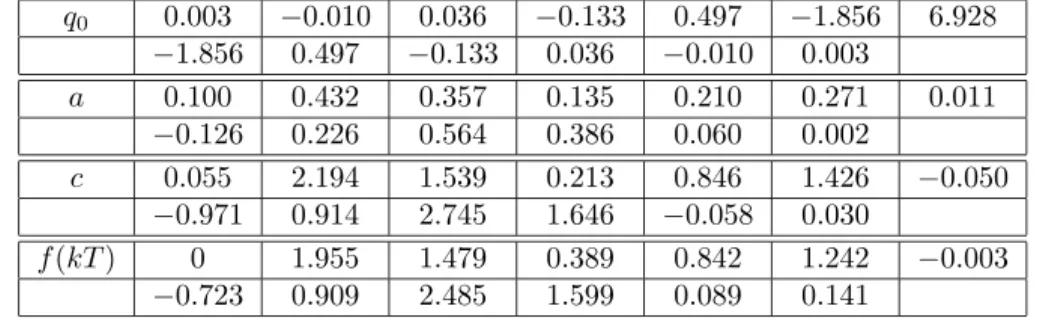
an interval containing [0,3]. In fact, an edge effect al-ways occurs, since the coefficients near the borders have been calculated without considering the contributions of the components of vectoraoutside the interval. Ta-ble 1 shows vectors q′
0, a and c for the example (only
13 nonzero elements were retained in rowq′
0, discarding
values lower than 10−3). The coefficients were computed
by numerical integration using the trapezoidal method. Since the aim here is only to have a pictorial represen-tation of the interpolation, values lower than 10−3were
neglected. Note thatq0is symmetric around the central value 6.928.
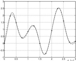
Figure 4 shows the signal recovered using the triangular basis. Note that the signal recovered does not necessar-ily fit exactly the sample valuesf(kT) and, moreover, the area between the actual function f(t) and its re-construction is smaller than the corresponding area in figure 2.
rep-Table 1: q0,aandcvectors forf(t) = sin(t) + sin(πt) + sin(2πt) and its sample valuesf(kT).
q0 0.003 −0.010 0.036 −0.133 0.497 −1.856 6.928 −1.856 0.497 −0.133 0.036 −0.010 0.003
a 0.100 0.432 0.357 0.135 0.210 0.271 0.011 −0.126 0.226 0.564 0.386 0.060 0.002
c 0.055 2.194 1.539 0.213 0.846 1.426 −0.050 −0.971 0.914 2.745 1.646 −0.058 0.030
f(kT) 0 1.955 1.479 0.389 0.842 1.242 −0.003 −0.723 0.909 2.485 1.599 0.089 0.141
0 0.5 1 1.5 2 2.5 3
-1 -0.5 0 0.5 1 1.5 2 2.5 3
t (s)
Figure 4: sin(t) + sin(πt) + sin(2πt) (dashed) and trian-gular series reconstruction (solid).
resented by the triangular pulses basis.
5
CONCLUSION
The main point in this paper was to highlight the re-lationship between the sampling theorem and the lin-ear interpolation process, using a convenient triangular pulse approximation for the sampling function.
The sample values f(kT) can be viewed as series coef-ficients on a basis of sampling functions. However, for the triangular series, the coefficients that minimize the quadratic error are not the sample valuesf(kT).
The calculation of the coefficients in the triangular basis is numerically involving, due to the nonorthogonality of the triangular pulses. The quadratic error is minimized, but the reconstruction of the function does not neces-sarily fit the signal atf(kT).
ACKNOWLEDGEMENT
This work was supported in part by “Conselho Nacional de Desenvolvimento Cient´ıfico e Tecnol´ogico” — CNPq, Brazil. The authors wish to thank the anonymous re-viewers for their valuable suggestions.
APPENDIX:
PROPERTY
OF
A
TRI-DIAGONAL MATRIX
Lemma: Consider the tri-diagonal matrix of dimension
M given by
BM =
b 1 0 · · · 0 0 0 1 b 1 · · · 0 0 0 0 1 b · · · 0 0 0 ..
. ... ... . .. ... ... ... 0 0 0 · · · b 1 0 0 0 0 · · · 1 b 1 0 0 0 · · · 0 1 b
(24)
with b > 2. As N → +∞, the central element aN of
matrixB−1
2N+1 converges to
aN → √ 1
b2−4 (25)
Proof: The central elementaN is given by
aN = [B2N+1]
−1 (N,N)=
d2N
d2N+1
= d
2
N
d2N+1
(26)
wheredN is the determinant of matrixBN. Moreover,
dN+2=bdN+1−dN , N = 1,2,3, . . . (27)
withd1=bandd2=b2−1. The eigenvalues of equation
(27) are
λ1=b+ √
b2−4
2 , λ2=
b−√b2−4
The solution of equation (27) is given by
dN =
λ1
λ1−λ2
λN
1 + λ2
λ2−λ1
λN
2 (29)
Sinceλ1>1 and 0< λ2<1, for N sufficiently large
dN ≈
λ1
λ1−λ2
λN
1 (30)
implying that
aN →
1
λ1−λ2 =
1 √
b2−4 (31)
REFERENCES
Burrus, C. S., Gopinath, R. A. and Guo, H. (1998). In-troduction to Wavelets and Wavelet Transformers: A Primer, Prentice-Hall, Englewood Cliffs, NJ.
Carlson, A. B. (1975). Communication Systems, 2nd edn, McGraw-Hill, Tokyo, Japan.
Chen, C. T. (1989). System and Signal Analysis, Saun-ders College Publishing, Orlando, FL.
Chui, C. K. (1997). Wavelets: A Mathematical Tool for Signal Analysis, Society for Industrial and Applied Mathematics, Philadelphia, PA.
Kwakernaak, H. and Sivan, R. (1991). Modern Signals and Systems, Prentice-Hall, Englewood Cliffs, NJ.
Lathi, B. P. (1965). Signals, Systems and Communica-tion, John Wiley & Sons, New York, NY.
Oppenheim, A. V., Willsky, A. S. and Young, I. T. (1983). Signals and Systems, Prentice-Hall, Engle-wood Cliffs, NJ.
Rabiner, L. R. and Schafer, R. W. (1978). Digital Pro-cessing of Speech Signals, Prentice-Hall, Englewood Cliffs, NJ.
Sinha, N. K. (1991). Linear Systems, John Wiley & Sons, New York, NY.