Diagnostic line profiles and modelling of the accretion and outflow regions around YSOs

(1)

Diagnostic line profiles

and modelling of the

accretion and outflow

regions around YSOs

Raquel Maria Galhofa de Albuquerque

Mestrado em Astronomia

Departamento de Física e Astronomia 2015

Orientadores

João José de Faria Graça Afonso Lima,

Professor auxiliar, Faculdade de Ciências da Universidade do Porto

Jorge Filipe da Silva Gameiro,

(2)

(3)

(4)

(5)

Acknowledgements

First and foremost, I would like to express my sincere gratitude to my supervisors Dr. João Lima and Dr. Jorge Gameiro, whose knowledge, support and guidance enriched further my master’s degree. Also, a very special thanks goes out to Dr. Véronique Cayatte and Dr. Christophe Sauty from the Astronomical Observatory of Paris, whose expertise, suggestions and patience taught me how to take my first steps in MHD numerical simulations. Without this incredible team of scientists, this thesis would not be possible. I am grateful to Centro de Astrofísica da Universidade do Porto for providing an office and technical support, specially from Paulo Peixoto who was tireless and very helpful regarding IT disasters and software details.

I would also like to thank all my friends for our random and singular moments, which helped me in several stressful scenarios. They know who they are (:

It is my privilege to thank Mia, Teresa, Fernando and Manel for their constant encouragement and friendship, which I cherish so much.

A special word of gratitude goes to Telmo, for being who he is and for all the good moments we have shared.

Last but not the least, I am deeply thankful to my family. Specially to my beloved parents, my dearest sister and my little nephew, for all their support, advice and fondness.

(6)

(7)

Abstract

Classical T Tauri stars (CCTS) are young solar-type stars that have been known by their enigmatic angular momentum evolution. In order for a Young Stellar Object (YSO) grow-up and maintain its equilibrium simultaneously, besides accreting matter, it also needs to eject part of it in the form of outflows (stellar winds, jets, magnetospheric ejections,...). By knowing how these accretion/outflow mechanisms occur and evolve, it will possible to better understand the origins of the Solar System.

CTTS have been studied both observationally and theoretically. Spectral observations allow astronomers to characterize these stars through mass, temperature, radius, accretion/outflow velocities and accretion rates that are encoded in their emission lines. On the other hand, theoretical studies provide analytical models through magnetohydrodynamics (MHD), which is the fundamental structure to develop steady and time-dependent numerical simulations. By figuring out the relevance of some physical quantities involved, it will be possible to replicate the observations made so far.

This dissertation will focus both on observational and theoretical perspectives. Firstly, I will explore some of the spectral features present in a sample of CTTS and infer about mass accretion rates and characterize their outflow dynamics. Secondly, I will discuss the results regarding the structure modelling of magnetospheres made with numerical simulations, in collaboration with Paris Astronomical Observatory researchers.

Keywords

Accretion, CTTS, MHD, Outflows, YSO

(8)

(9)

Resumo

As estrelas T Tauri clássicas (CTTS) são estrelas jovens do tipo solar conhecidas pela enigmática evolução do seu momento angular. Para um objeto estelar jovem (YSO) crescer e manter o seu equilíbrio em simultâneo, além de acretar matéria, necessita também de ejetar uma parte sob a forma de outflows (ventos estelares, jatos, ejeções magnetosféricas,...). Ao saber como estes mecanismos de acreção/ejeção ocorrem e evoluem, será possível compreender melhor as origens do Sistema Solar.

As CTTS têm vindo a ser estudadas tanto observacionalmente como teoricamente. As observações espectrais permitem aos astrónomos caracterizar estas estrelas através da massa, temperatura, raio, ve-locidades de acreção/ejeção de matéria que estão codificadas nas suas riscas de emissão. Por outro lado, estudos teóricos fornecem modelos analíticos através da magnetohidrodinâmica (MHD), que é a estrutura fundamental para desenvolver simulações estacionárias e dependentes do tempo. Ao descobrir a relevância de algumas quantidades físicas envolvidas, será possível replicar as observações realizadas até hoje.

Esta tese será direcionada numa perspetiva observacional e teórica. Em primeiro lugar, irei explorar algumas das características espectrais presentes numa amostra de CTTS e inferir acerca de taxas de acreção e caracterizar a dinâmica de ejeção de matéria. Em segundo lugar, irei discutir os resultados relativos à modelação de magnetosferas feitas a partir de simulações numéricas, em colaboração com investigadores do Observatório Astronómico de Paris.

Palavras chave

Acreção, CTTS, MHD, Outflows, YSO

(10)

(11)

List of Figures

1.1 Illustration of the star-disk interaction . . . 17

2.1 Position of T Tauri stars on an Hertzprung-Russel diagram . . . 23

2.2 Spectral differences bettween a CTTS and a WTTS . . . 24

3.1 Accretion mechanism in T Tauri stars . . . 28

3.2 Schematic view of accretion/outflow mechanisms in CTTS . . . 29

3.3 Representation of different outflow mechanisms . . . 29

3.4 Representation of morphologies of winds and jets . . . 30

3.5 Representation of a steady-state X-wind model . . . 32

3.6 Temporal evolution for magnetospheric ejections . . . 33

3.7 DG Tau microjet . . . 34

3.8 Illustration of jets in T Tauri stars. . . 35

3.9 Representation of magnetic star-disk interaction . . . 37

3.10 Representation of stellar winds, magnetospheric ejections and disk-winds . . . 37

4.1 Representation of the definition of equivalent width. . . 41

4.2 Equivalent widths determination . . . 41

4.3 Equivalent width correlation for various line combinations . . . 44

4.4 Reipurth et al. (1996) classification scheme for Hα emission line profiles . . . 47

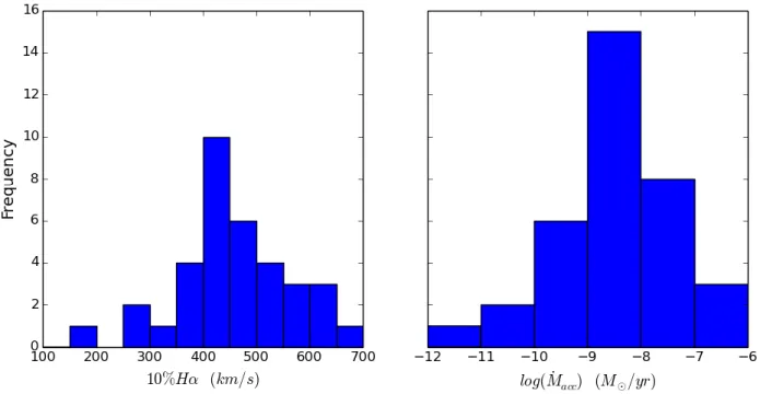
4.5 Histograms for the equivalent width and mass accretion rates for Hα line . . . 48

4.6 Velocity profiles for He I lines λ5876 and λ6678 . . . 53

4.7 Velocity plots for forbidden lines . . . 55

4.8 Zoom-in in velocity plots for forbidden lines . . . 56

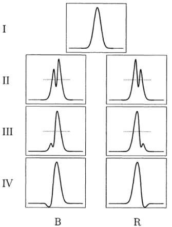
4.9 Illustration of Type III P Cygni profile . . . 58

4.10 Distribution of emission peak velocities . . . 59

4.11 Correlation of the fitted velocities for He I λ5876 and λ6678 . . . 61

4.12 Histograms for the parameters determined in the 3GF . . . 65

5.1 Representation of gas flows in a star-disk magnetic system . . . 68 13

(14)

5.2 Illustration of two self-similar field line structures . . . 70

5.3 Representation of the Alfvénic cylindrical radius . . . 74

5.4 Representation of the poloidal velocity inversion . . . 78

5.5 Representation of the shift between analytical and simulated poloidal velocities . . . 80

5.6 Plots for Test001_03 . . . 82

5.7 Plots for Test001_04 . . . 83

5.8 Plots for Test001_05 . . . 84

5.9 Plots for Test001_05 . . . 85

5.10 Plots for Test003. . . 86

5.11 Plots for Test004 and Test005 . . . 87

5.12 Plots for Test006 and Test006_01 . . . 92

5.13 Plots for Test009_01 . . . 93

5.14 Plots for Test009_02 . . . 94

5.15 Plots for Test009_02 . . . 95

5.16 Plots for Test009_03 . . . 95

5.17 Plots for Test009_06 . . . 96

5.18 Plots for Test009_07 . . . 97

5.21 Mass flux vs poloidal velocity for Test011 . . . 100

5.22 Plots for Test012. . . 101

5.23 Density plots for Test013 . . . 101

5.24 Mass flux and poloidal velocity plots for Test013 . . . 102

6.1 Representation of mass flux (log(ρ|Vp|)) for the analytical solution . . . 105

6.2 Mass fluxes for the best simulations . . . 108

6.3 Kelvin Helmoltz instabilities in Saturn atmosphere . . . 110

A.1 Triple gaussian fitting for Hα λ6563 . . . 128

A.2 Triple gaussian fitting for He I λ5876 . . . 131

(15)

List of Tables

4.1 Determination of radial velocities . . . 43

4.2 Determination of equivalent widths for different chemical elements . . . 45

4.3 Determination of equivalent widths and mass accretion rates for the Hα line . . . 52

4.4 Triple gaussian fitting for Hα emission line . . . 62

4.5 Triple gaussian fitting for He I λ5876 emission line . . . 63

4.6 Triple gaussian fitting for He I λ6678 emission line . . . 64

5.1 PLUTO code simulations . . . 89

6.1 Mass flux determinations . . . 107

(16)

(17)

Chapter 1 Introduction

“Astronomy, as nothing else can do, teaches men humility.” — Arthur Clarke

T Tauri stars (TTS) are pre-main sequence objects of low mass (≤ 2M1) with ages between 1 and

10 million years, when they become optically visible. The classical T Tauri stars (CTTS) are surrounded

by a circumstellar accretion disk from which they gain mass near ∼ 10−8_M

/yr and have mass-loss

rates around 10−9_M

/yr (see figure 1.1). Also, they exhibit very strong magnetic activity, based on

observations of strong X-ray emission and the detection of dark star spots covering large fractions of the

stellar surface (Ferreira, 2013;Hartmann, 2009; Petrov et al.,2014).

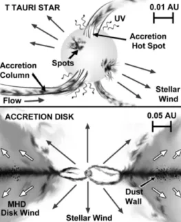
Figure 1.1: Adapted illustration of the star-disk interaction by Matt and Pudritz (2005a). The material migrates from the exterior to the inner region of the circumstellar disk and it is channelled to the polar region of the star through the accretion columns. Disk and stellar winds are outflow processes that are associated with accretion mechanisms in young active stars. The dashed and dash-dotted lines indicate the location of the Alfvén surfaces in the stellar and disk winds, respectively.

According toBouvier et al.(2007), the intensity-weighted mean magnetic field strength over the surface

of most T Tauri stars analysed is ∼ 2.5 kG in the photosphere. Therefore, magnetic fields on TTS are

much stronger than on the Sun ∼ 500 G (Aschwanden,2005).

1_{Solar mass, where 1M}

∼ 1.9891 × 1030kg

(18)

Observational data shows that these young stellar objects (YSOs) are very active during the pre-main sequence stage, due to the presence of strong winds and jets which are thought to be driven by accretion mechanisms. Moreover, the most powerful winds can be observed on FU Orionis stars (FU Ori), which show episodic outbursts of several magnitudes related with dynamical instabilities. These stars are spectrally

characterized by a large mass loss rate ( ˙M = 10−5M/yr), broad photospheric lines and luminosity

of a supergiant. In addition, angular momentum transfers intensifies as well as accretion and outflow

mechanisms (Petrov, 2003; Petrov et al., 2014).

Theoretically, we would expect that YSOs would spin up due to accretion and contraction processes, but that is not observed. Two possible angular momentum removal mechanisms can be considered according to Matt and Pudritz (2005a): winds and jets formed in magnetohydrodynamic (MHD) processes. The angular momentum of the star is regulated by the magnetic star-disk interaction, in which the large scale open magnetic field connects the rotating star-disk system with the circumstellar medium, and the magnetized outflowing gas removes the mass and angular momentum from the system.

Emission line profiles are used to study the dynamics of the circumstellar medium, namely the motion of the gas in a stellar wind or the accretion of gas to a star. Evidence of the outflow of matter (absorption shifted to shorter wavelengths, the so-called P Cygni profiles) can be found in Hα, while indications of accretion (absorption shifted to longer wavelengths, inverse P Cygni profile) are observed in the profiles

of He I, for instance (Petrov, 2003). Although forbidden lines, as [OI] and [SII], do not present any P

Cygni profiles, their emission is also associated with outflow processes. Emission line profiles encode not only geometrical but also physical information on the accretion/outflow processes and its rate. One of

the main challenges is to use those line profiles to understand both mechanisms (Bouvier et al., 2007).

Through mass accretion rates is possible to understand disk structure and evolution, as well as planet

formation and migration (Calvet et al.,2004). Furthermore, estimates of the accretion mass can already

be provided through the equivalent width and the width measured at 10% peak intensity of the Hα line (Natta et al., 2004), Paschen and Brackett lines (near-infrared) and veiling. For the latest, in CTTS the lines of the photospheric spectra are less deep than in normal stars of the same spectral type and the absorption spectrum appears weak and veiled. This veiling is caused mainly by additional continuum

emission of nonphotospheric origin, which increases toward shorter wavelengths (Petrov, 2003).

At the moment, there is no model capable of simulate alone all the physical mechanisms involved in YSOs, due to its complexity and interactivity. Nevertheless, models may be built and constrained according to observations in a first approach.

Sauty and Tsinganos (1994) developed a semi-analytical MHD model to simulate outflow mechanisms observed among YSOs. The mentioned model uses the meridional self-similar approach, which simplifies the set of partial MHD differential equations into nonlinear ordinary ones, through variable separation and

function scaling with one of the spatial coordinates, the colatitude θ (Sauty et al., 1998). The latest

(19)

FCUP 19 Diagnostic line profiles and modelling of the accretion and outflow regions around YSOs

magnetospheric accretion processes, which are thought to feed outflow mechanisms. The results obtained throughout the numerical simulations made with PLUTO code will be explored and discussed.

Regarding the thesis structure, in chapter 2 is given a short review regarding T Tauri stars general features, folllowed by section 3 where accretion and outflow mechanisms are described as well as angular momentum extraction processes known. Chapter 4 and 5 show the results regarding observations and simulations, respectively, and chapter 6 makes the linkage between these two last perspectives. Finally, conclusions are drawn in chapter 7.

(20)

(21)

Chapter 2 T Tauri Stars

2.1 UNVEILING T TAURI STARS

The best approach we have, in order to understand the evolution of the solar system, is to study young solar-like forming stars. These low mass, pre-main sequence (PMS) stars can be found in stellar nurseries, are named T Tauri stars (TTS) and are classified as class II objects.

TTS were named after the discovery of the first star with the same characteristics: T Tauri. The star was discovered in October of 1852 by an asteroid hunter, John Russel Hind, who was scanning the night sky and found out that this star was missing from the charts of stars with magnitude 10. Due to its

photometric variability, it was not observed and catalogued earlier1_.

The infrared (IR) excess observed in young stellar objects can be seen as a measure of stellar youth and can be quantified through the infrared spectral index given by

αIR ≡

d log(λFλ)

d log(λ) , (2.1)

where λ is the wavelength and λFλ is the flux measured per logarithmic wavelength interval, typically

between 2.2 and 10 µm. According to different αIR values, pre-main sequence stars are classified with

different classes (Lada and Wilking,1984; Adams et al., 1987; Stahler and Palla, 2005):

• Class 0: sources deeply buried only detected at far-infrared and millimeter wavelengths;

• Class I: αIR > 0, these objects are associated with dense cores;

• Class II: −1.5 < αIR< 0, are less embedded stars, namely classical T Tauri stars (CTTS);

• Class III: αIR < −1.5, correspond to brighter stars which circumstellar disk has been dispersed and

the accretion processes, when observed, are very weak (weak line T Tauri stars - WTTS).

1_{American Association of Variable Star Observers:}

http://www.aavso.org/vsots_ttau

(22)

Regarding variability, T Tauri stars were first identified byJoy(1942) as a group with variable brightness

(also know as irregular variables). Ambartsumian (1947) found that TTS occur in groups named

T-associations, which have a connection with O-associations (groups of OB stars). He suggested that TTS were the low-mass counterpart of recently formed OB stars. Later, TTS were subdivided in two groups: CTTS still accreting from their circumstellar disks and WTTS without a disk (do not show NIR excess)

and with weak Hα emission lines (Herbig, 1962; Herbig and Bell, 1988; Hartmann, 2009). While CTTS

seem to be more irregular, WTTS show periodic photometric variations. The weakly variability among

CTTS has three possible causes according with Grankin et al. (2007): cold surface spots (resulting from

strong magnetic fields), hot surface spots (associated with disk accretion onto the star) and variable obscuration of the star by the circumstellar disk.

Thanks toAmbartsumian(1947), TTS can be seen as a proof that star formation processes still continue

in our Galaxy. These stellar objects have their origin in gravitational collapses on molecular clouds. Once hydrostatic equilibrium is reached, accretion mechanisms are still active and the star is wrapped by an opaque cloud, which optically hides the protostar. The star becames visible in the optical when the protostar reaches the T Tauri stage. Here, besides accretion, outflow mechanisms are also observed and are thought to be responsible for slowing down the rotation velocity of these objects. In addition, before the star reaches the main sequence through the Hayashi track, gravitational energy is the main source of energy. In this descending “path”, the star is mainly convective and keeps approximately its temperature, while the luminosity decreases. Afterwards, a radiative core begins to form and this time luminosity is kept constant while temperature rises until is sufficient to the helium ignition, starting nuclear reactions and marking the entry in the main sequence. The remains of the accretion disk will be accreted

into planetesimals and afterwards a whole new set of orbiting planets is formed. Figure 2.1 shows the

distribution of T Tauri stars in the Hertzprung-Russel diagram. It is possible to observe that these stars

are located at the right of the main sequence in the regions of convective and radiative tracks (Petrov,

2003).

In the 1990’s, observations in the IR accused not only the presence of circumstellar disks around T Tauri stars but also that they are interacting with the central star through accretion mechanisms. The IR luminosity of the disk is caused both by re-radiation of light from the central star and by its own radiation (Lynden-Bell and Pringle,1974; Petrov,2003).

While CTTS have a typical rotation period of 6-9 days, WTTS show a value between 2-5 days (Bouvier

et al.,1995). CTTS rotate more slowly than WTTS due to the magnetic interaction between the accretion disk and the central star. When the disk begins to dissipate (star goes from CTTS phase to WTTS), the star begins to speed up and dynamo processes can be expected to become even stronger. In other words, WTTS represent the intermediate stage between the accretion phase and the zero-age main sequence (ZAMS). In addition, all the high energy mechanisms involved affect the remaining of the circumstellar disk material (protoplanets and planetesimals included) and may be relevant to understand observable

(23)

Figure 2.1: Position of T Tauri stars on an Hertzprung-Russel diagram byPetrov(2003). Are represented evolution tracks for stars with 0.4M, 1.0Mand 2.0M(solid lines) along with three isochrones for ages 105, 106and 107years (dashed lines).

properties of asteroids in the solar system (Audard et al., 2005).

(24)

2.2 SPECTRAL FEATURES IN CTTS AND WTTS

Accretion and outflow mechanisms govern many spectral features among young stars and are

funda-mental in the star formation process (Hartigan et al., 2004). Classical T Tauri stars are more active

than weak line. While CTTS present accretion disks responsible for the spectra excess in the UV and IR, pronounced stellar winds and rich emission-line spectrum ( Hα, H and Ca II, for example); WTTS do not

have accretion disks and only magnetic activity occurs (see figure 2.2).

Figure 2.2: Medium-resolution spectra of three T Tauri stars. The received flux is correct only for BP Tau while the remaining spectra were shifted vertically. V830 Tau is a weak line T Tauri star, while BP Tau and DR Tau are classical T Tauri stars. For the most active stars, DR Tau and BP Tau, it is possible to observe some relevant emission lines as Hβ and Hα, at 4861Å and 6563Å respectively (Stahler and Palla,2005).

TTS are dwarf stars with deep convective zones and their photospheric spectra ranges from late F to

M, but their typical spectrum is K7 V (Herbig,1962; Cohen and Kuhi,1979). Usually, TTS show a great

number of photospheric absorption lines, but they vary according to spectral type and can be diluted by

veiling (Reipurth et al., 1996).

What distinguishes TTS from main sequence stars is the ultra-violet and optical continuum excess emission, also known as veiling. The intensity of this spectral feature increases towards shorter wavelengths,

suggesting its origin from a hot region with gas at 104_{K. When looking to CTTS spectra, the photospheric}

lines appear to be less deep and weak (therefore, veiled). This excess manifests also in the Balmer jump

emission at 3646Å. According to Herczeg and Hillenbrand (2008), the size of the Balmer jump tends

to increase with both decreasing stellar mass and accretion rate. Veiling is usually attributed to the presence of an additional continuum emission of nonphotospheric origin. It has been discussed that the observed hot continuum emission could arise from the dissipation of accretion energy of hot spots, where magnetospheric gas shocks rapidly onto the stellar surface. Hence, measurements of this excess can

provide estimates for mass accretion rates (Muzerolle et al.,1998b;Stahler and Palla,2005;Petrov,2003;

(25)

Veiling (r) is also one way to measure stellar youth and its given by

rλ = Fveilλ /Fphotλ , (2.2)

where Fλ

veil is the flux of the veiling continuum (given by F∗λ − Fphotλ , where F∗λ is the measured flux of

the star) and Fλ

phot is the flux of the undisturbed photosphere (Muzerolle et al., 1998b). Hartigan et al.

(1995) showed that the heavily veiled CTTS are on average younger than the remaining stars in the sample

studied.

Analysing figure 2.2, is possible to observe that V830 Tau (WTTS) is less veiled than BP Tau and

DR Tau (both CTTS), which show shallower lines and less absorption dips. Heavily veiled stars have their spectra dominated by emission produced by accretion, with rare photospheric component and dense

emission lines at higher wavelengths (Herczeg and Hillenbrand, 2014).

When looking to a TTS emission spectrum, it is quite similar to the chromosphere of the Sun (Joy,

1945). In the optical band it is possible to detect pronounced emission lines for Hα. In the near IR

band, the most intense lines are from the Ca II triplet (8498, 8542 and 8662 Å). In the IR, it is possible to observe Paschen and Brackett series lines. Regarding features in the mid-IR and far-IR bands, those belong to the stellar wind and circumstellar dusty disk. In addition to this set of features, CTTS have also

Balmer series lines and lines of neutral and singly ionized metals (Petrov, 2003).

Emission line profiles are key factors regarding the study of circumstellar dynamics, namely gas motion in stellar winds and accretion mechanisms. For instance, when matter is being ejected from a star by jets or winds (outflows), the Hα absorption line is shifted to shorter wavelengths and acquires the so-called P Cygni profile. When matter is being accreted, absorptions are shifted to longer wavelengths, jointly with the formation of inverse P Cygni profiles, among the higher members of Balmer series, He I and Fe II (Stahler and Palla, 2005;Petrov, 2003).

It is worth to mention that intense stellar winds and accretion are only observed in CTTS. Also, forbidden emission lines of [OI] and [SII] are mainly observed in these type of pre-main sequence stars. Although these lines have lower intensities than allowed ones, their emission comes from rarefied gas flows (i.e. jets/winds) at distances higher than 1 AU from the star. When studying forbidden lines, among the majority of TTS is possible to observe double profiles. There is a central emission peak at the radial velocity of the star, that can be slightly shifted to the blue, and an emission peak between -50 to -150

km/s with origin in a stellar wind and/or in a jet (Petrov,2003).

2.3 MAGNETIC FIELDS IN TTS

T Tauri stars show evidence of strong magnetic activity, due to the presence of X-ray emission (Feigelson

et al.,2007), which is higher three orders of magnitude than the solar corona, the presence of large starspots (Herbst and Shevchenko,1999) and indirect measurements of large photospheric magnetic fields (

(26)

Krull et al., 1999). Magnetic field intensities in these stars can reach values between 1-2 kG, which is

sufficient to channel accretion flows (Hartmann, 2009; Petrov et al., 1976).

X-ray emission has been observed both in WTTS and CTTS and depends on the rotation velocity of the stars. Among CTTS, X-ray emission is related to accretion mechanisms, while in WTTS is associated

with magnetic activity due to a dynamo mechanism as in main-sequence magnetically active stars (Audard

et al., 2005).

Concerning stellar spots, cold spots can be observed in WTTS and CTTS and have areas between 5−10% of the stellar surface and temperatures within the range 200 − 1200 K (lower than the photosphere). In contrast, hot spots are only observed in CTTS, cover only 1 − 2% of the stellar surface, have temperatures

between 7000 − 10000 K and exist no more than a few revolutions of the star (Herbst et al.,1994;Petrov,

2003). Photometric studies suggest they are the source of additional radiation responsible for the veiling

of the photospheric spectrum. Due to the fact that these spots are only observed in CTTS, which have circumstellar disks from which they gain mass, these features may be caused by the gas accretion on the

surface of the star (Bouvier and Bertout,1989). Herbst et al.(1994) confirmed this idea with a correlation

(27)

Chapter 3 Star-disk interaction

From the accretion neutron star model of Ghosh and Lamb (1979), Uchida and Shibata (1985) and

Koenigl (1991) adapted it to explain the low rotation periods observed among active TTS. One of the main ideas in the star-disk interaction is that, in order for T Tauri stars truncate their disk at a radius

bigger than the stellar radius (between 3 and 7R∗), they must have strong dipolar fields (between 1 and

3 kG) and maintain the connection between the accretion disk and the star. In other words, the disk is truncated where the magnetic field pressure balances the ram pressure of the accreting material. In addition, this magnetized interaction would have a fundamental impact regarding the transfer of angular momentum back to the disk. Also, the infalling of material from the disk onto the stellar surface guided

by magnetospheric fieldlines (with associated mass accretion rates between 10−9 _{and 10}−7_M

/yr), could

explain the UV excesses found in observations (Bouvier et al., 2007;Ferreira, 2013).

This star-disk interaction results in a balance between accretion and outflow mechanisms. According to

Hartigan et al.(1995), the ratio between mass loss and accretion is approximately 1%. More specifically,

Cabrit(2007) infer that typical ratios of jet mass flux to accretion rate for low-mass CTTS are near 10%. In both cases, this means that accretion processes are the dominant effect.

3.1 ACCRETION

The evolution of circumstellar disks has become increasingly important since the boom discovery of exoplanets and respective planetary systems. By studying accretion and outflow mechanisms in these set of young accreting stars, in the future it will be possible to derive more clues regarding the evolution of

stars and planet formation scenarios (Bouvier et al., 2007).

In agreement with Kepler’s laws, the accretion disk material rotates differentially. Due to the fact that rotation energy is converted to thermal energy by the viscosity, the temperature of the disk increases and radiation is emitted. Meanwhile, matter descends to lower orbits, as it loses energy, until being accreted.

(28)

Disks usually last for ∼ 2 − 5Myr, have sizes about 100 AU and the temperature at 10 AU is around 100 K. They can also be classified as active or passive. Active refers to self luminous accretion disks, while passive refers to disks that re-radiates absorbed starlight in the IR. This distinction can be made through luminosity. When considering passive disks, the observed bolometric luminosity for the star-disk system should be the same as for a star of the same spectral type. In the case of active disks, the luminosity of

the disk may be higher than the star (Herczeg and Hillenbrand, 2014; Petrov, 2003).

Figure 3.1: Illustration of the accretion phenomenon in T Tauri stars (not to scale) byStahler and Palla(2005).

In figure3.1 the magnetospheric accretion mechanism is illustrated. The stellar object is surrounded by

an accreting circumstellar disk which emits at several wave bands, namely: infrared, sub-mm and mm. In the inner disk, the stellar magnetic field lead to its disruption by transferring disk material onto the star. This magnetospheric material emits broad emission lines (namely Hα line) along the infalling accretion columns, producing a hot continuum when crashing onto the stellar surface originating the so-called hot

spots (represented in figure 3.2). The truncation radius is located inside the radius at which dust is

sublimated by radiation from the central star and accretion shock (Stahler and Palla, 2005).

Mass accretion rates can be seen as a disk evolution indicator since it usually decreases with time as mass

is accreted onto the star (Hartmann, 2009). According to Calvet et al. (2004), the best determinations

(29)

Figure 3.2: Schematic view of accretion/outflow mechanisms in CTTS byFrank et al.(2014).

3.2 OUTFLOWS

Outflows are the reverse process of accretion and can be easily observed in stellar or galactic objects (Petrov, 2003; Tsinganos, 2007). They can be shaped in uncollimated winds and collimated jets, with bipolar flows oriented in two opposite directions and perpendicular to the plane of the disk. When flows are driven by more narrow and compact bipolar streams, they are designated jets and can be supported

by Hα, [NII], [OI] and [SII] emission lines (Petrov,2003).

Besides jets, stellar winds are also an outflow phenomenon (see figure 3.3) with mass flux rates near

10−9M/yr. This mechanism can be detected in TTS spectra through blueshifted absorptions among

Hα and Ca II (for example), in which velocities range from 100 to 400 km/s.

Figure 3.3: Representation of stellar winds (blue), X-winds (pink) and magnetospheric accretion (green) processes location in a YSO. Figure adapted fromFerreira(2013).

Another configuration for outflows is based on the conical wind model proposed by Romanova et al.

(2009), were mass is transferred from the inner disk and accelerated by magnetic pressure.

When studying outflow regions, forbidden line profiles provide useful informations regarding its

(30)

tion, namely the existence of two velocity components: a fast (> 100 km/s) and a slow one (< 50 km/s). The first case refers to a narrowly directed jet, while the second one is supposed to be related with an

outflow of matter from the surface of an accretion disk (Hartigan et al.,1995;Kwan and Tademaru,1988;

Petrov, 2003).

According to Sauty et al. (1998), some of the most intriguing questions concerning outflows are the

acceleration mechanisms and their various morphologies. For the latest, it has been suggested that winds

and jets expand conically and cylindrically, respectively (see figure3.4).

Figure 3.4: Illustration of winds (left) and jets (right) morphologies bySauty et al.(1998).

Stellar winds

Since the 1980’s that stellar winds, similar with the solar case, have been pointed out for their importance

regarding angular momentum extraction among young accreting stars (Shu et al., 1988; Hartmann and

Stauffer, 1989). The accretion rate is proportional to the amount of angular momentum carried onto the star by the disk. Therefore, stellar winds could be a key factor to slow down the rotation period of the star due to accretion when the outflow rate is approximately 10% of the accretion rate, as expected

theoretically by some authors (Hartmann and Stauffer, 1989; Matt and Pudritz, 2005a). Additionally,

Cabrit et al.(1990) concluded that stellar winds in TTS are correlated with accretion, due to Hα and IR luminosities, respectively.

According to Matt and Pudritz (2005a), part of the gravitational potential energy released during

accretion could be powering stellar winds and boosting mass outflow rates. In addition, the associated torque increases not only with magnetic field strength, but also with the mass loss rate. Furthermore, the authors introduced the Accretion Powered Stellar Winds paradigm (APSW). In the latest, the stellar dipolar

field truncates the disk at Rt, imposing the matter to accrete onto the star, through the magnetospheric

(31)

compressive waves in the star photosphere. The turbulent process would be able to convert part of the resultant thermal and kinetic energy to MHD turbulence which could supply kinetic energy to stellar winds formation.

Because the latest model establishes a direct relation between accretion and ejection,Zanni and Ferreira

(2011) thought that accretion shock luminosity LUV could be used to constrain the wind characteristics

and give upper limits to the spin-down efficiency. The authors found out that luminous sources with

LUV ≥ 0.1Land typical dipolar field components lower than 1 kG do not allow spin equilibrium solutions.

In addition, lower luminosity stars (LUV < 0.1L) are compatible with a zero-torque condition, which

contrasts with the high necessity of mass and energy for stellar winds. For such matter, its argued that the APSW is not efficient to explain the spin-down observed among CTTS.

Gregory et al. (2012) and Zanni and Ferreira (2013) have shown that the stellar magnetic field is not sufficient to produce relevant stellar winds. An efficient spin-down torque requires a rather strong dipolar component, which is rarely seen among classical T Tauri stars. The authors suggest that non-axisymmetric and multipolar magnetic components should be considered when studying torques acting on the protostar and they must be consistent with observations.

An important aspect to take into account is that there must be an upper limit for the ratio between the mass loss rate and mass accretion rate, otherwise there will not be sufficient energy to drive stellar

winds. Matt and Pudritz (2008) suggested that the ratio should be approximately ˙Mwind/ ˙Macc 6 60%.

Despite all the progress made so far, how accretion power may transfer to a stellar winds still needs further investigation.

X-winds and disk winds

The purpose of the X-wind model theorized by Shu et al. (1994) was to explain YSO jets as well as

the spin-down of the protostar. According to the authors, X-winds have their origin in the inner region of the disk and should be the dominant factor in YSO jets (concerning mass flux, appearance and power) responsible for angular-momentum extraction, such that the star is not spun up by accreting material (Ferreira, 2013).

In order to explain the slow rotation periods of accreting T Tauri stars, the X-wind model takes into

account the interaction between the stellar disk and the stellar magnetosphere. Figure 3.5 illustrates the

X-wind model for the steady-case scenario. Initially, the stellar magnetic flux that threads the entire disk is captured in the X-region, which is a narrow annulus located at the disk inner edge. In the latest region the magnetic pressure prevails over gas pressure, such that the annulus rotate as a solid body. In addition,

it contains the corotation radius RX (3 − 5R∗ for TTS, e.g. Hartmann(2009)), where the stellar angular

velocity is equal to the Keplerian angular velocity: Ω∗ = ΩX = pGM∗/R3X. This implies that disk

material near the interior radius RX rotates at sub-Keplerian velocities, which enables the disk material

to flow through the fieldlines (bended inwards) onto the star. On the other hand, disk material near the

(32)

exterior radius RX will rotate at super-Keplerian velocities, such that it will ascend along the fieldlines (bended outwards) and escape in a wind.

Regarding angular velocity,Artemenko et al.(2012) discovered that it remains constant when considering

CTTS with 0.3 to 3M and ages between 1 and 10 Myr, suggesting the existence of an efficient angular

momentum regulation mechanism. Moreover, completely convective (less massive) CTTS rotate slower than CTTS on radiative evolutionary tracks (more massive) and the majority of CTTS have periods no longer than 10 days.

There is an excess of angular momentum transferred from accretion to the disk material in the inner portion of the X-region, which will tend to push the material outwards. In contrast, induced disk winds (launched from the extended disk region) in the outer portion of the X-region will transfer angular mo-mentum to outflowing gas at the expense of the disk material connected by fieldlines with origin in the exterior of the X-region, pushing this material inwards. This outward and inward push on the inside and outside region of the X-region will conduct to the so called trapped flux phenomenon and to the disk truncation at the inner edge. Taking all into account, the angular momentum transfer from accretion

funnels to the wind lead to a slow rotation of the star (Bouvier et al.,2014;Ostriker and Shu, 1995).

Another interesting feature in figure 3.5 is the helmet streamer structure, which is formed through the

interface between open field lines loaded with outflowing matter (connected to the disk) and those not loaded (connected to the star). Along these features, major mass ejection and reconnection events may

arise in response to changes in the boundary conditions (Ostriker and Shu, 1995).

Figure 3.5: Representation of steady-state X-wind model by Bouvier et al. (2014). The black thick line represents the truncated disk and the black solid curves the magnetic fieldlines. The purple dotted line shows the co-rotation radius RX

and the purple thick line represents the X-region. Red and blue arrows show the direction of mass and angular momentum transport, respectively. Green arrows refer to the pinching of gas is the X-region due to angular momentum transport.

(33)

Magnetospheric ejections

Magnetospheric ejections (MEs) can exchange mass, energy and angular momentum with the star and the disk. This exchange begins with an expansion followed by reconnection of the closed magnetospheric lines connecting the star to the disk. The inflation process develops through the star-disk differential

rotation and resultant build-up of toroidal magnetic field pressure (Zanni and Ferreira, 2013). According

to the authors, the angular momentum exchange with the star is mainly controlled by the differential rotation between the star and the MEs. If at the cusp of the fieldline the mass loaded from the disk rotates more slowly (faster) than the star, the MEs exert a spin-down (spin-up) torque.

At more distant regions from the star, MEs disconnect from the central region of the disk-star region in a magnetic reconnection event and propagate ballistically as magnetized plasmoids (much alike coronal mass ejections in the Sun) in a channel delimited by two quasi-steady MHD flows: the inner stellar wind

and an outer disk wind (see figure3.10). Due to magnetic reconnection, the inner magnetic surfaces close

again (see figure3.6) and this magnetic slingshot mechanism repeats along the time in a quasi periodically

way (Bouvier et al., 2014; Ferreira,2013; Zanni and Ferreira, 2013).

Figure 3.6: Temporal evolution of the periodic inflation/reconnection process of magnetospheric ejections powered by stellar and disk rotation. Blue arrows represent the poloidal velocity vectors and the white lines the magnetic fieldlines. Are also represented logarithmic density maps with and the yellow solid lines follow the evolution of a single magnetic surface showing the dynamics of the phenomenon. Time is given in units of rotation periods of the central star (Zanni and Ferreira,2013).

Zanni and Ferreira (2013) concluded that MEs are partly responsible for controlling the rotation period of a star. They are able to efficiently extract angular momentum from the disk close to the truncation region such that the spin-up accretion torque is considerably reduced. Furthermore, and due to differential rotation, MEs can extract directly angular momentum from the star if the ejected plasma rotates slower than the star. Furthermore, the authors discovered that the combined effect of MEs and stellar wind lead to the spin-down torque on the star. For such matter, MEs could be one of the best mechanism to explain the disk-locking phenomenon observed in CTTS.

Jets

Although the precise origin of jets from YSOs is still being discussed, is accepted that the ignition process

involves the interactive dynamics of accreted matter with stellar and/or disk magnetic field (Frank et al.,

(34)

2014). However, it is not defined if jets have their origin from the stellar surface (Sauty and Tsinganos,

1994), the magnetosphere/disk interface (Shu et al., 1995) or a wide range in disk radii (Ferreira,1997).

In figure 3.7 are shown small jets detected in a CTTS. This kind of images provides the opportunity to

test current ejection theories, because they not only give access to the interior wind regions (≤ 100AU) but also give information concerning stellar and accretion properties. Besides images to study non-relativistic

jets in YSOs, position-velocity diagrams, emission lines, mass accretion rates are also useful tools (Ferreira,

2013).

Figure 3.7: Deconvolved [OI] 6300Å plus the narrow-band image of DG Tau microjet through adaptive optics (Dougados et al.,

2004)

Jets are highly collimated structures (opening angle of a few degrees) composed by bright separate nodes caused by pulsed acceleration of the jet of a young star. In addition, a bright arc (bow shock) may

form where the collimated flow collides with the interstellar medium, as illustrated in figure 3.8 (Petrov,

2003). Moreover, jets can carry between 5 × 10−10 _{and 2 × 10}−8_M

/yr, which according to Schwartz

(1983) andMundt (1988), is suggest that only a small fraction of the stellar wind is collimated into jets.

More specifically for CTTS, typical outflow rates vary between 10−9 _{and 10}−7_M

/yr (Frank et al.,2014).

When observing jets in the optical wavelength, its only possible to trace one side of the jet outflow (towards the observer in the blueshifted side), while the other one is traced in the NIR emission in

molecular hydrogen and radio observations, which are unaffected by extinction (Hartmann,2009). Hence,

observations proved that YSO jets are bipolar, but interestingly, despite of ejecting the same amount of

mass at each jet, terminal velocities may differ by up to a factor of 2 (Podio et al.,2011; Melnikov et al.,

2009).

The observed jets among CTTS have regions of forbidden line emissions with sizes between 100 and 500

AU and carry velocities near 170 km/s (Hirth et al.,1996). Interestingly, around half of the observed pair

of opposite jets seem to present different velocities. This means that jets are not being equally accelerated (Hirth et al.,1994b; Woitas et al.,2002). To support these ideas, observations have shown that jets may

suffer strong disturbances due to shocks and possibly unsteady ejections events from the star (Ferreira,

2013). Moreover, and according to Frank et al. (2014), a jet may be seen as a string of shocks with a

wide range conditions.

(35)

et al. (2000). Because jets are essentially a time-dependent phenomenon evidenced by their knotty morphology, steady-state models are a good starting point to study them under a theoretical perspective.

There are already three main model types for YSO jets: stellar winds (Sauty et al.,2004;Matt and Pudritz,

2005a), X-winds (Shu et al.,1994;Cai et al., 2008) and magnetized winds (Blandford and Payne, 1982;

Ferreira and Pelletier, 1993; Ferreira and Casse, 2004). Although they are based on different boundary conditions, they all share the same MHD equations and existence of a strong magnetic field in a rotating

object (Ferreira, 2013).

Figure 3.8: Illustration of jet features in T Tauri stars in two different scales byFrank et al.(2014).

3.3 ANGULAR MOMENTUM EXTRACTION

As mass, temperature and metallicity, the angular momentum of a PMS star is one of the most

funda-mental physical quantities, which characterizes the rotation and translation of a body: ~L = ~r×~p = ~r×m~v.

The rotation of a star influences not only its internal structure, energy transport, mixing processes in the

stellar interior, but also its magnetic activity (Bouvier et al., 2014).

By studying the evolution of the angular momentum along the lifetime of the stars, questions concerning star formation processes, accretion/outflow mechanisms in YSOs, future of stellar activity and its impact

on planetary formation could be answered (Bouvier et al., 2014).

One of the big questions is why are YSOs showing values for their rotation velocity lower than the

ones expected theoretically. Looking to the solar case and according to Priest (1984), the velocity of the

solar-wind plasma is inclined about 1.5◦ relatively to the radius vector. This is going to translate in a

deceleration effect in the rotation of the Sun, due to the fact that angular momentum is being transferred from the Sun to the solar wind. In a similar way, this process will also occur in PMS stars but in a more pronounced level due to stronger magnetic fields and pronounced accretion/outflow mechanisms.

Stars with disks are slower rotators when compared with diskless ones. While the former ones have

(36)

rotation periods between 3 to 10 days, the later ones show periods between 1 and 7 days, which can be

photometrically derived from monitoring surface spots (Bouvier et al., 2014).

In addition, it seems to exist a trend between stellar mass and rotation periods. According toHerbst et al.

(2001) and Cody and Hillenbrand (2010), observational data suggests that rotational braking becomes

gradually less efficient towards stars with lower masses (M∗ < 1M).

Gallet and Bouvier(2013) suggest that the evolution of spin rates of solar-mass stars requires substantial angular momentum loss at nearly all stages of evolution and the required amount of torque is higher in the young forming ages. And the largest torques could be explained by the fact that a substantial fraction of

stars with ages below 5 Myr are still accreting through a star-disk interaction (Koenigl,1991). Therefore,

the dissipation of the disk (which corresponds to the cessation of accretion processes) could explain the

transition to weaker torques. Zanni and Ferreira (2013) concluded that, depending on the accretion rate,

magnetospheric ejections can extract a relevant amount of accretion torque and, together with a weak but non-negligible stellar wind torque, can balance the spin-up due to accretion.

The disk-locking process, initially proposed byGhosh and Lamb(1979), has been verified by observations

and suggests that stars, during the first million years in the PMS, are interacting with their disks through the magnetic field. The model is confirmed by the inverse relationship between the angular velocity of

the star and the near-infrared excess, suggesting the presence of a circumstellar disk (Artemenko et al.,

2012).

According to figure3.9, only if outer radius Rout (the outermost radial extent of the magnetic connection)

is bigger than co-rotation radius Rco (where the Keplerian angular velocity is equal to the stellar angular

velocity), magnetic braking and accretion will occur. As mentioned previously for X-winds, fieldlines connecting the disk outside the co-rotation radius will have a spin-down effect, while the fieldlines coupled to the disk inside will have the opposite effect. Hence, to enable accretion in the pre-main sequence stars,

the truncation radius (Rt) needs to be smaller than the co-rotation radius (Rt < Rco). Once again in

figure3.9, in the interior region to Rt, the disk material will be confined to the stellar fieldlines, will carry

the same angular velocity as the star and material is accreted to magnetospheric columns. Outside Rco

the stellar angular velocity is super-Keplerian, therefore material locked to the stellar field may experience

a centrifugal force which will lead to an outer star-disk region (Matt and Pudritz, 2005b; Bouvier et al.,

2007).

The presence of outflows such as stellar winds, magnetospheric ejections and disk-winds could also explain and/or complement the efficient angular momentum extraction from a star-disk system with a

dipolar magnetosphere. In figure 3.10 three types of outflows in a star-disk system are represented:

stellar winds accelerated along the open magnetic flux anchored onto the star, magnetospheric ejections associated with expansion and reconnection processes of closed magnetic fieldlines connecting the star and disk-winds (including X-winds) launched along the open stellar magnetic surfaces threading the disk (Bouvier et al., 2014; Zanni and Ferreira,2013).

(37)

Figure 3.9: Illustration of the magnetic star-disk interaction byMatt and Pudritz(2005b). From the truncation radius Rt to

the outer radius Rout, that region of the disk is connected to the star through the accretion flow (arrow).

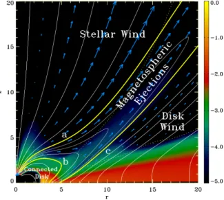
Figure 3.10: Representation of a star-disk interacting system with three different dynamical constituents of the system: (a) stellar winds, (b) magnetospheric ejections and (c) disk-winds. A logarithmic density map is shown in the background. Blue arrows represent poloidal velocity vectors. The dotted line marks the Alfvén surface and the white lines represent the field lines

(Zanni and Ferreira,2013).

The magnetic star-disk interaction, besides their effect on the star angular momentum evolution and the inner structure of the disk, could also have an important role regarding the migration of young planets

close to the central object (Lin et al.,1996). The authors suggest that initially a planet forms at a greater

distance from the star (∼ 5 AU), and afterwards it subsequently migrates inwards through interactions with the remnants of the circumstellar disk. Moreover, tidal interactions with the star, or through truncation of the inner circumstellar disk by the stellar magnetosphere, may be responsible for interrupting the migration of the planet in its present orbit.

(38)

(39)

Chapter 4 Diagnostic line profiles

The observational study and analysis of this thesis project started with a sample of 58 reduced échelle spectra of T Tauri stars taken by António Pedrosa (from 1998 November 7 to 9) with UES (Utrecht Echelle Spectrograph) at the 4.2 m William Herschel Telescope, installed at the Spanish Observatorio del Roque de los Muchachos of the Instituto de Astrofísica de Canarias, on the island of La Palma. All spectra were originally wavelength-corrected for heliocentric velocity and normalized to a continuum level of unity.

When modelling accretion and outflow mechanisms, the strength and profile of the emission lines reveal

to be useful tools (Fernandez et al.,1995). The spectra of CTTS includes emission line profiles that can

give hints regarding outflow/accretion signatures. According to White and Basri (2003) classification,

each star of the sample was classified as classical (if Wλ(Hα) > 10Å, where Wλ is the equivalent width)

or weak line (if Wλ(Hα) < 10Å). Subsequently, the sample was reduced to 38 CTTS, the most active

stars. In these selected sample, three stars were discarded: V510 Cas, V1082 Cyg and V1331 Cyg. In the first case, it was the most noisy spectrum in all the sample. The second star was discarded because the spectral type was not defined in many references. The spectrum of V1331 Cyg is a continuum spectrum with emission lines, therefore due to the lack of photospheric absorption lines, it was not possible to make the radial velocity determinations.

Because the spectra were already corrected from the heliocentric velocity, it was only necessary to make a final correction from the radial velocity (RV). The corrections adjust the stars observed velocity from the rotation and translation motions of Earth. In order to determine radial velocities for each spectrum,

were used two routines from IRAF1 _{(see table} _4.1_{). The fxcor routine determines radial velocities}

through Fourier cross correlation by giving as inputs the spectrum of the star, a template (in the stellar rest-frame) and respective apertures of the échelle spectrum with less noise and strong emission lines. The rvidlines routine calculates the radial velocities through the determination of wavelength shifts in spectral lines relative to specified rest wavelengths. Contrary to fxcor, rvidlines does not give any

1_{Image Reduction and Analysis Facility:}

http://iraf.noao.edu/

(40)

associated error.

Later, from the two radial velocities obtained the best one was picked up to make the correction. In order to make this selection, for each observed spectra were added/subtracted, separately, each radial velocity value determined by the two routines and compared with a simulated spectra (template). The

selected velocity (marked with an asterisk in table 4.1) was the one for which the shift would lead to an

approximate/coincident overlap of photospheric lines between the observed and simulated spectra. Once the correction was done, the spectra were finally transformed into the stellar rest frame.

Taking all into account, most of the radial velocity corrections were made using the values obtained through fxcor routine. The rvidlines routine returned in many cases negative velocities contrasting with the positive ones determined by fxcor and available in the literature. This negative sign could be a result of applying the rvidlines routine in noisy spectra. Probably, IRAF identified noise as spectral lines given to make the comparison. One way to deal with this problem could be the selection, of the given list of spectral lines, according to less noisy wavelength intervals. When comparing the chosen RVs with the ones documented in the literature, some values are quite proximate namely for AA Tau, BP Tau, DL Tau, DQ Tau, DS Tau and GK Tau, for instance.

Besides radial velocity determinations, equivalent widths for different chemical elements were measured through IRAF’s splot routine, namely: Hα 6563Å, Hβ 4861Å, He I 5876Å, Ca II triplet (8498, 8542 and

8662Å), Paschen line P11 8863Å, [OI] 6300Å, [SII] 6731Å and OI 7772Å listed in table4.2. For the latest

element, some inverse P Cygni (IPC) profiles were detected and indicated in the table, but they are not very strong.

The equivalent width is a quantitative tool to measure the strength of a line in emission/absorption.

Considering an absorption line in figure 4.1, the equivalent width Wλ is given by an integral over the line

Wλ ≡

Z

(1 − Fλ/F0)dλ, (4.1)

where Fλ and F0 are the specific flux received from the star and the continuum flux on either side of the

absorption dip, respectively. According to the last figure, this quantity can be interpreted as the width of a hypothetical line with rectangular profile, that represents the same integrated flux deficit from the

continuum as the true one (Stahler and Palla, 2005).

For the Hα line, the equivalent width measurements were compared later with the values determined

through a Python2 _{script (see figure} _4.2 _{and table} _4.3_{). The equivalent width is more dependent of}

the continuum normalization than signal to noise ratio (S/N), which measures the strength of the signal relatively to background noise. For such matter, the error for the equivalent width of Hα was

deter-mined considering the corresponding values above and below 1% of the continuum (Wλ+1% and Wλ−1%,

2

(41)

Figure 4.1: Representation of the definition of equivalent width for an absorption line (Stahler and Palla,2005).

respectively):

Error Wλ(Hα) =

1

2(|Wλ− Wλ+1%| − |Wλ− Wλ−1%|) , (4.2)

where Wλ is the equivalent width measured along the continuum.

(a)AS 353A (b)BP Tau

Figure 4.2: Determination of equivalent widths for Hα emission line through a Python script for AS 353A (P Cygni profile) and BP Tau (gaussian-like profile). The green and magenta horizontal line marks 10% of the maximum intensity of the line and the continuum, respectively. Red and blue vertical lines mark the widths of the line at 10% of the maximum intensity and at the continuum, respectively.

Whenever two emission lines are well correlated, they are probably formed in the same region. For such

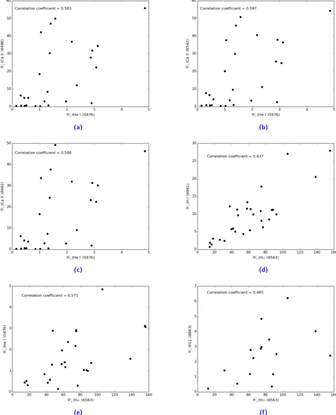
matter, correlations between different line elements were made. In figure4.3 were plotted the correlations

for various lines including Hα 6563Å, Hβ 4861Å, He I 5876Å, Ca II 8498, 8542, 8662Å and P11 8863Å.

In figures 4.3e and 4.3f, there is a low correlation between the line strengths of Hα with He I and Hα

with P11. In contrast, in figure 4.3d, Hα and Hβ show the strongest correlation (Pearson correlation

coefficient = 0.837), suggesting a common emitting region.

(42)

Muzerolle et al. (1998b) suggest that Ca II triplet lines are good indicators of accretion rates. The remaining plots correspondent to He I and Ca II triplet correlations, are somewhat less correlated at higher line strengths, as seen by the latest authors. Line profiles for Ca II triplet were not studied in

detail for this thesis, but according to Hamann and Persson (1992), in these lines a broad and a narrow

component can be identified. While the broad emission component is thought to come from an extended envelope with large turbulent velocities (apart from the stellar surface), the narrow component results from

chromospheric activity in the star. For the latest, Batalha et al. (1996) suggest that the emission comes

from the chromospheric active regions correlated with local concentration of fieldlines generated by stellar dynamo (the product of the combined effect between stellar differential rotation and subphotospheric

convection). Later,Azevedo et al. (2006) besides suggesting that the narrow component fluxes may come

from a hot chromosphere, they can also have their origin in accretion shock or wind, while the fluxes from the broad component are probably formed in the magnetospheric accretion flow.

Probably, the low correlation between He I and Ca II triplet seen in figure 4.3 may be related not only

with different origin from He I, but also with the distinct origins for the two components in the Ca II triplet, as seen previously. Another important factor to take into account is veiling. Since the continuum excess is wavelength dependent, it will be more relevant for He I (at a lower wavelengths) than for Ca II (at higher wavelengths). Because the analysed spectra were not veiling corrected, variations in the continuum excess will probably lead to variations in the equivalent width of the lines and affect the correlations made.

In table 4.2 are listed the equivalent widths measured for He I λ5876, Hα λ6563 and OI λ7772, and in

table4.3 are shown the determined accretion rates throughNatta et al. (2004) empirical relationship for

the Hα line (described in the following section). As seen previously in figure 4.3e, there is a correlation

between Hα and He I λ5876, where Wλ(Hα) values increase with Wλ(He I). Additionally, when comparing

these two last lines with OI λ7772 and the determined accretion rates, it is possible to observe that, in a

few cases, higher accretion rates are associated with OI in absorption (Wλ > 0), including IPC profiles.

For instance, the highest value verified for ˙Macc corresponds to 10−6.18 M/yr for RW Aur, which has the

highest absorption measured for OI within an IPC profile. In contrast, AA Tau presents lower equivalent

widths, including OI in emission, and the lowest value among accretion rates, 10−11.31_M

/yr. It should

be mentioned that these results could be influenced by the star inclination relatively to the observer and veiling. One way to obtain a proper correlation could be analysing the corresponding fluxes and/or luminosities for all the lines.

(43)

Table 4.1: Radial velocity determinations for each star identified in the 1st _{column. In the 2}nd

column are shown the spectral types, the 3rd _{column shows the radial velocity values available in}

the literature. 4th _{and 5}th _{columns correspond to radial velocity determination through IRAF’s}

fxcor routine and associated error, respectively. In the last column are shown the radial velocities determined with rvidlines routine. The chosen RVs for the correction are followed by an asterisk.

Object Spectral type RV_lit RV_{f xcor} Error RV_{f xcor} RV_rvidlines

(km/s) (km/s) (km/s) (km/s) AA Ori K4i _18.8q _25.3∗ _0.7 _26.7 AA TAU K7t _17.1b _16.8∗ _0.6 _16.4 AS 353A K2t _−12.1p _−7.9∗ _1.9 _−10.0 BM And K5a ₋₂₇k _−8.1∗ _2.5 _−5.7 BP Tau K7a _16.18c _17.8∗ _1.6 _18.0 BZ Sgr K0Ver _−5.4r _−1.7∗ _6.0 _0.6 CI Tau K7a 16.2r −57.9 4.8 1.4∗ CW Tau K3a _{16.4 ± 1.3}j _30.8 _2.0 _26.7∗ DF Tau M2a ₁₂g _172.5 _6.4 _9.7∗ DG Tau K6a _17.9f _−26.9 _7.9 _21.2∗ DI Cep G8a ₋₁₀g _−12.6 _3.3 _−11.5∗ DK TAU K7a _15.3j _19.2∗ _2.0 _20.4 DL Ori K1e _? _24.2∗ _2.2 _−61.7 DL Tau M0a 16l 17.9∗ 1.6 −35.0 DQ Tau K7-Ms _22.4n _22.7∗ _0.9 _22.6 DR Tau K7a _16.5f _23.3∗ _0.7 _−22.7 DS Tau K5i ₁₃l _14.2∗ _1.1 _7.6 EH Cep K2i ? −19.7 1.8 −9.5∗ GK Tau K7a _{18.6 ± 1.4}j _17.6∗ _1.4 _14.7 GM Aur K7a _{15.0 ± 1.3}j _15.9 _0.9 _13.7∗ LkHα 191 K0a ? −7.1∗ 0.4 −7.3 LkHα 330 G2t 20k 15.1 1.2 6.4∗ RW Aur K2a _{14.0 ± 4.9}j _15.9∗ _2.1 _3.6 RY Tau K1a _17.8f _7.7 _2.2 _20.4∗ T Tau K0a 23.9g 18.6 0.6 17.4∗ UY Aur K7a ₁₈d _16.2∗ _1.3 _23.7 UZ Tau E M1.3i _{2.8 − 36.8}m _18.5 _3.1 _17.3∗ V1079 Tau K5t _? _17.4 _0.6 _16.3∗ V1305 Ori K5e _? _28.9∗ _2.2 _25.9 V1980 Cyg Gi _? _−8.6∗ _3.1 _4.4 V466 Ori K1t 23.2j 34.3 1.7 27.9∗ V625 Ori K6i _? _−20.9 _2.4 _−16.9∗ V649 Ori G8III – K4Vs ₃₆l _27.4∗ _1.8 _21.9 V828 Cas K1i _? _−0.7∗ _0.8 _−1.2 WY Ari K5t ₉k _−5.9∗ _2.7 _−7.6

References: a -Artemenko et al.(2012); b -Bouvier et al. (2003); c -Chubak and Marcy(2011);

d -Edwards et al. (1987); e -Fang et al.(2009); f - Gahm et al.(2005); g -Gontcharov(2006);

h -Gramajo et al. (2014); i -Grankin et al.(2007); j -Hartmann et al. (1986); k -Herbig(1977);

l - Joy (1949); m - Martín et al.(2005); n -Mathieu et al. (1997); o - Petrov et al.(2014); p

-Rice et al.(2006); q - Tobin et al.(2009); r -Torres et al. (2006); s - The International Variable

Star Index (http://www.aavso.org/vsx/index.php); t - SIMBAD (http://simbad.u-strasbg. fr/simbad/).

(44)

(a) (b)

(c) (d)

(e) (f)

Figure 4.3: Equivalent width Wλcorrelation between He I λ5876 and Ca II λλ8498, 8542, 8662, Hα λ6563 with Hβ 4861, He

I λ5876 and P11 λ8863. All measurements were made in angstroms and the Pearson correlation coefficients are mentioned at the top-left corner of each plot.