The performance of accounting-based valuation methods in the presence of dirty surplus flows, an empirical analysis and a practical insight on Broker’s reports

THE PERFORMANCE OF ACCOUNTING-BASED VALUATION

METHODS IN THE PRESENCE OF DIRTY SURPLUS FLOWS, AN

EMPIRICAL ANALYSIS AND A PRACTICAL INSIGHT ON

BROKER’S REPORTS

Thesis submited to Lancaster University and Católica Lisbon School of Business and Economics in the fulfilment of the requirements of the double degree of Master in Science in Finance

by

Nuno Maria Moura Tavares de Carvalho Martins

B. Sc. in Management and Business Adminstration (CLSBE, Portugal)

September, 2012

08

Fall

2

THE PERFORMANCE OF ACCOUNTING-BASED VALUATION METHODS IN

THE PRESENCE OF DIRTY SURPLUS FLOWS

,

AN EMPIRICAL ANALYSIS AND A

PRACTICAL INSIGHT ON BROKER’S REPORTS

Nuno Maria Moura Tavares de Carvalho Martins

B. Sc. in Management and Business Adminstration (CLSBE, Portugal)

Thesis submited to Lancaster University and Católica Lisbon School of Business and Economics in the fulfilment of the requirements of the double degree of Master in Science in Finance

September, 2012

ABSTRACT

This dissertation analyzes the performance of accounting-based valuation methods in the

presence of dirty surplus flows. We will first perform an empirical analysis on a large sample

of U.S. companies between 2005 and 2010. This analysis compares the performance in

terms of valuation errors of different accounting-based valuation methods (RIVM, AEGM and

P/E) between two groups, with low and high level of dirty surplus flows. The study will show

that P/E as the best accounting-based valuation method and it is independent of dirty surplus

flows presence, while, RIVM was the second-best valuation method, followed by AEGM. The

influence of dirty surplus flows is found in both RIVM and AEGM models. Particularly, the

study reports that the longer the forecast horizon, the higher the valuation error AEGM would

produce, in the presence of higher level of dirty surplus flows.

Then a small sample of broker’s reports from FTSE 100 was studied. The study was divided in three parts; Studying the importance of dirty surplus for brokers, Practical insights about

the valuation models used by brokers and Understanding the relevance of dirty surplus flows

information to brokers. Brokers who introduce dirty surplus flow information in the valuation

model, would, on average, use the DCF valuation model. However, the study concludes that

the majority of brokers do not consider dirty surplus flow information. Finally, reports that

incorporate dirty surplus flows information tend to achieve better performance. This

dissertation presents JP Morgan reports as an example.

08

Fall

3

Acknowledgements

First I want to acknowledge Lancaster University and Católica-Lisbon School of Business and

Economics for the key role that both universities played by inspiring me, developing my

analytic skills and motivating me to think further. Also, I would like to especially thank all the

professors and staff members that accompanied and supported me throughout my master

degree.

I would like to give my supervisor, Professor Ricardo Reis, a special word of appreciation for

all the help; without him this project would never have been finished.. Thank you as well to

Professor Zhang Gao, Christian Stadler and Professor John O´Hanlon for their advices.

This project would never have existed without the support of my best friend, Sofia Bento

Monteiro. I thank her for being a constant and special presence in my live throughout the

years and for always visiting me wherever I went.

Thank you to all my friends for this unforgettable year in Lancaster. A special

acknowledgement to the wolf pack for being my family in Lancaster. Zhang Ping, Luke

Hobson and Michael Joyner. Jessica Chen and Zhau Lu you were like my parents, in a good

way. Nann I want to thank you for making this year so special.

Last but not least, I would like to sincerely thank all my family for the unconditional support

that they gave me, especially to my closest relatives. First and foremost to you mum, for

committing all your life to us, for being an example of dedication and for calling me every

single day in order to know how everything was going. Thank you Ana, even though from

Brazil, our skype conversations were like a breath of fresh air, making it possible to face this

project. Moreover, in the last month your “presence” was essential. Brother, your visit to Lancaster was very special and the continuous calls where key to keep me on track, a

sincere thank you. Finally I would like to thank you dad. Thank you, for all the motivational

4

List of Contents

ABSTRACT ... 2

ACKNOWLEDGEMENTS ... 3

LIST OF CONTENTS ... 4

ABBREVIATIONS ... 6

LIST OF TABLES ... 7

LIST OF APPENDICES ... 9

CHAPTER 1. INTRODUCTION ...10

CHAPTER 2. LITERATURE REVIEW ...12

I.

T

HE

I

MPORTANCE OF

A

CCOUNTING

N

UMBERS IN

V

ALUATION

... 12

II. V

ALUATION PERSPECTIVES

... 13

III. M

ULTIPLES

V

ALUATION

... 14

Choice of Value Driver ... 14

Comparables Firms Selection ... 15

Benchmark Multiple Calculation ... 16

Advantages and Disadvantages of Multiples Valuation ... 17

IV. D

IVIDEND

D

ISCOUNT

M

ODEL

... 17

I.

R

ESIDUAL

I

NCOME

V

ALUATION

M

ODEL

... 19

II. A

BNORMAL

E

ARNINGS

G

ROWTH

V

ALUATION

M

ODEL

... 21

VIII.

T

HE

E

QUIVALENCE

B

ETWEEN

RIVM

AND

AEGM ... 21

CHAPTER 3. LARGE SAMPLE ANALYSIS - THE PERFORMANCE OF

ACCOUNTING-BASED VALUATION METHODS IN THE PRESENCE OF DIRTY SURPLUS FLOWS, AN

EMPIRICAL ANALYSIS ...23

I.

I

NTRODUCTION

... 23

I.

D

ATA COLLECTION

... 25

5

III. S

AMPLE

S

ELECTION

... 25

IV. D

IRTY

S

URPLUS

F

LOWS AND

V

ALUE

E

STIMATE

C

ALCULATION

... 27

V. T

HE PERFORMANCE OF ACCOUNTING

-

BASED VALUATION MODELS IN THE PRESENCE OF DIRTY SURPLUS FLOWS

... 27

VI. R

OBUSTNESS TESTS

... 31

Growth rate of Terminal Value ... 32

Cost of Equity Capital ... 32

CHAPTER 4. SMALL SAMPLE ANALYSIS - A PRACTICAL INSIGHT ON BROKERS'

REPORTS ...37

I.

I

NTRODUCTION

... 37

II. D

ATA COLLECTION

... 38

III. P

ERIOD

C

OVERED

... 38

IV. S

AMPLE

S

ELECTION

... 38

V. D

IRTY

S

URPLUS

F

LOWS IN BROKER

’

S REPORTS

... 39

VI. D

IRTY

S

URPLUS

F

LOW RELEVANCE IN BROKER

’

S REPORTS

... 43

VII. JP

M

ORGAN CASE STUDY

... 45

CHAPTER 5. CONCLUSIONS ...52

APPENDIX 1 – THE DERIVATION OF RIVM FROM DDM ...54

APPENDIX 2 – THE DERIVATION OF AEGM FROM DDM ...56

APPENDIX 3 – THE EQUIVALENCE BETWEEN RIVM AND AEGM ...58

APPENDIX 4 – DIRTY SURPLUS FLOWS AND VALUE ESTIMATE CALCULATION ...61

D

IRTY

S

URPLUS

F

LOWS

C

ALCULATION

... 61

V

ALUE

E

STIMATE

C

ALCULATIONS

... 63

Cost of Equity ... 64

Residual Income Valuation Model ... 64

Abnormal Earnings Growth Model ... 66

Price to Earnings multiple ... 67

6

Abbreviations

AEGM – Abnormal Earning Growth Model BVPS – Book Value Per Share

CSR – Clean Surplus Relationship DCF – Discounted Cash Flow DDM – Dividend Discount Model Dow – Dow Jones Industrial Average EBIT – Earnings Before Interest and Tax

EBITDA – Earnings Before Interest, Tax, Depreciation and amortization EPS – Earnings Per Share

FASB –Financial Accounting Standard Board I/B/E/S - Institutional Broker’s Estimate System NYSE – New York Stock Exchange

P/E – Price to Earnings Ratio 𝑅𝐸– Residual Earnings

RIVM – Residual Income Valuation Model SIC – Standard Industrial Classification TDSF – Total Dirty Surplus Flows

7

List of Tables

Chapter 3

Table 3.1 – Summary of the Sample Selection Process of Large Sample Analysis Table 3.2 – Summary statistics of primary variables of Large Sample

Table 3.3– Summary statistics of descriptive variables of Large Sample by Group Table 3.4– Summary statistics of input variables of Large Sample

Table 3.5 – Signed and Absolute valuation errors for the entire sample Table 3.6 – Signed and Absolute valuation errors by group

Table 3.7 – Median Signed paired test for RIVM and AEGM2

Table 3.8 – Mean paired t-test for absolute valuation errors of AEGM5 and AEGM2 Table 3.9 – Mean sample t-test in signed and absolute terms for all the models Table 3.10 – Median two-sample test in signed and absolute terms for all the models

Table 3.11 – Regression analysis of value estimates and share price for all the models by group

Chapter 4

Table 4.1 – Small sample summary

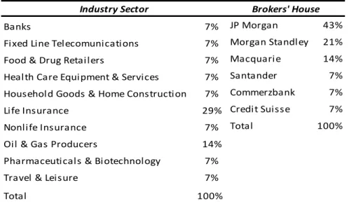
Table 4.2 – Company, valuation date and broker’s house of the reports selected Table 4.3 – Industry sector and Broker’s house analysis

Table 4.4 – Valuation Model used by brokers Table 4.5 – DSF in the Broker’s reports

8

Table 4.7 – Absolute and Signed Valuation Error by Group

9

List of Appendices

Appendix 1 – The derivation of RIVM from DDM Appendix 2 – The derivation of AEGM from DDM

Appendix 3 – The Equivalence between RIVM and AEGM Appendix 4 – The Equivalence between RIVM and AEGM

10

1. Introduction

“Violation of the clean surplus relationship (CSR) may result in mismeasurement of performance and value”

(Isidro et al., 2004)

Clean Surplus Relationship (CSR) is a structural concept in Accounting and Finance theory.

Feltham and Ohlson (1995) describe CSR as a relationship, which assumes that there will be

no items affecting directly equity without passing through the income statement. Assuming

that CSR holds, the final book value of equity is equal to the initial book value of equity plus

net income minus dividends. In this case, a perfect articulation between the balance sheet

and the income statement exists. However, in reality what happens is that the majority of the

companies report comprehensive income statements. These accounts are known as Dirty

Surplus Flows (DSF), For example: gains and losses resulting from currency translation,

marketable securities adjustments or pension liabilities adjustments. Consequently, CSR

does not hold any more, which raises the problem of incorrect measurement of performance

and value. This problem derives from earnings use in the valuation process. In fact, the

earnings figure is regarded as a summary indicator of a company’s financial performance and value-creation, Isidro (2005). However, since some gain and losses bypass the net income

and are directly accounted in equity, an incorrect measurement might occur.

Moreover, the importance of dirty surplus flows to valuation depends on the expected

persistence and magnitude of it throughout time. For example, if investors expect that it is just

a one off situation with expected small magnitude, it will not affect future dividends and it

might not affect valuation. On the contrary, if higher magnitude and persistence over time is

expected, valuation might be affected if dirty surplus flows are excluded.

Previous academic researches (O’Hanlon and Pope (1999), Biddle and Choi (2002) and Isidro et al. (2006)) already acknowledged this issue. However, no previous research has

examined the possible interaction between dirty surplus flows magnitude and

accounting-based valuation models performance. This thesis investigates this exact matter. An algorithm

to calculate the total amount of dirty surplus and the calculation of valuation errors to measure

the performance of the different accounting-based valuation methods is used to generalize

11

It’s also essential not only, reaching academic conclusions but understanding what is done in practical terms. However, the previous research seems to be missing this.

By incorporating in-field experiences of brokers, we could deeply understand the issue and

might be able to generate a new understanding of this problem. To bridge the gap between

academic theory and practice, I would continue my analysis by studying, how the broker’s reports consider DSF information. The case study of JP Morgan will be used as practical

example.

In short, this thesis aims to study the influence of the dirty surplus flow magnitude in

accounting-based valuation models performance and investigate what is the common

practice. This could contribute to further academic knowledge by complementing the

discussion about dirty surplus and its implications between the three circles: academics,

professionals and investors.

This thesis is divided in 5 chapters. First of is Literature Review, then in Chapter 2 I approach

the two valuation perspectives. After that the three accounting-based valuation models used

in this thesis, Multiples, RIVM and AEGM are discussed. I address the advantages and

disadvantages of each one and relate the different research findings.

Large sample analysis is present in chapter 3. This chapter analyses the performance of the

different accounting-based valuation models in the presence of dirty surplus flows. I explore

the difference of performance (in valuation errors terms) of the different accounting-based

valuation models between a group with high level of DSF and a group with low level of DSF.

Chapter 4 presents the small sample analysis. This analysis studies the link between DSF

and broker’s reports. I look in detail at specific examples in order to understand the relevance of DSF in practice. Finally, the conclusions of this thesis are presented in chapter 5.

12

2. Literature Review

Analysts, individual investors, shareholders and academics have a common interest:

determining what is the accurate value of a specific firm. From finance theory, in an efficient

market, the value of a specific firm equals the expected value of future cash flows discounted

at the appropriate discount rate (Copeland et al., 2003).

In order to calculate the value of a specific firm, individuals need the support of reliable

information. It could be argued that share price might be a good approximation, however, it is

not enough. There are a significant number of companies that are not listed, therefore

making it impossible to use share prices to calculate its value. Furthermore, the share price

represents what you have paid for that specific firm while the value represents what you get.

This ambiguity lead previous researches to test the market efficiency hypothesis, trying to

understand if prices fully reflect the information available about the company. Frankel and Lee

(1998) concluded that: ‘‘price convergence to value is a much slower process than prior evidence suggests”.1

I. The Importance of Accounting Numbers in Valuation

In this case, in a valuation process, the information contained in the financial statements of

the company under valuation becomes an extremely relevant part, although, the financial

statements are not the only source that will be used. Financial Accounting Standard Board

(“FASB”) conceptual framework has the objective of help investors and creditors in

“assessing the amounts, timing, and uncertainty” of accounting numbers (FASB, 1978). This way, the firm value can be calculated more accurately. Although FASB objective was not

equity valuation, the conceptual framework reinforces the relevance and leaves no doubt

about the significant importance of accounting numbers to realize the valuation of a company.

Before that academic researches discussed the importance of accounting numbers. Beaver

(1968) concludes that individual and market expectations are different when earnings values

are announced. Ball and Brown (1968b) found that more than 50% of the new available

1Another examples of research testing market hypothesis are Fama (1970), Foster et al. (1984), Bernard and Thomas (1989), Ball and Bartov (1996), and Kraft (1999).

13

information is reflected in the income numbers. More recently, Lee (1999) emphasized the

importance of accounting numbers, classifying it into three major roles: language for

forecasting, helpful information and finally to serve as ex post settling-up mechanisms.

II. Valuation perspectives

While understanding the importance of accounting numbers individuals usually face a

bottleneck when evaluating a company; the choice of the evaluation model. Belonging to a

group which does not invest following their intuition, individuals consider fundamental analysis

has an anchor in the valuation process.2 Meaning; analyzing information about the company, as its financial statements, and based on that information calculating the intrinsic value of the

firm (Graham and Dodd, 1934)3.

In fundamental analysis one distinction must be made, whether we use an entity or equity

valuation. Entity valuation consists in the comparison of the value driver (e.g., EBITDA or

invested capital) with the market value of the entire firm, not just equity. Since the valuation is

trying to capture all the value created to the entire firm, the value driver should be a

performance measure attributable to the entity as a whole. In opposition, equity valuation

refers to value drivers (e.g., earnings or book value), which are attributable only to equity. The

decision to use either perspective depends on the situation in analysis. On entity valuation the

firm is being evaluated as a whole rendering the accounting and financing policies almost

insignificants. Consequently, this perspective is easy to use in international comparisons,

although, it involves a more detailed forecasting analysis by the user. On the other hand,

equity valuation is easy to calculate and is used worldwide, which facilitates the comparison.

However, due to management-financing decisions affecting it, the utility is reduced, Citigroup

Global Markets (2005).

Analysts, shareholders, individual investors and academic researchers apply a variety of

different accounting-based valuation models. In the following sections I analyze in detail

2Examples of research in fundamental analysis are: Beaver et al. (1980), Ou and Penman (1989), Stober (1992), Kothari and Zimmerman (1995), and Piotroski (2000)

3 The book “Security Analysis” from Graham and Dodd have recently been publish as

_“

Graham and Dodd's Security Analysis” by Cottle et al.

14

Multiples, Residual Income Valuation Model (RIVM) and Abnormal Earnings Growth Model

(AEGM).

III. Multiples Valuation

Comparables or Multiple Valuation consists on the multiplication of a value driver from the

company being evaluated (e.g., book value or earnings) by the corresponding benchmark

multiple. The benchmark multiple is the ratio of the value driver used by the stock price, for a

group of comparable firms (Penman, 2004). Therefore, the traditional method of multiple

valuation could be represented by the following equation:

4

(1)

The summarizes the group of comparable firms (Liu et al., 2002). The different methods of calculation the benchmark multiple are presented later on.

Choice of Value Driver

However, some empirical researches demonstrate that individuals can use some anchors in

the value driver selection process. The first hint is that forward multiples are superior to

trailing ones. As pointed out before the valuation of a company is based on the expected

future cash flows. As such, it is predictable that the correlation of forecasted drivers, for

example earnings and the expected payoffs tend to be higher than the correlation using

trailing multiples. Academic researches demonstrated this result. Liu et al. (2002) while

analyzing the valuation performance of different value drives, both in terms of individual

industry and in terms of cross industry, found that forward earnings multiples explain better

the price of a firm in both types of analysis, increasing as well the performance of the

valuation if the period of forecasting is extended. That argument was reinforced by Lie and

4Where represents estimate value of the firm stand for the value driver of thecompany _, which have to be positive_{( ).}

15

Lie (2002) and Jing Liu et al. (2007), which show that forecasted earnings-based valuations,

for a significant part of the companies under analysis, are notably more accurate.

In relation to value driver selection, Tasker (1998) concluded that the preferences in terms of

value drivers by practitioners are conditioned by the industry under analysis.5 Supporting this,

Fernández (2002) said “it is also true, depending on the industry being analyzed, that certain multiples are more appropriate than others”, for example in the Bank industry the most common use multiple is Price to Book Value while in the Leisure industry it’s the Enterprise Value to EBITDA. The author justifies that these findings are related to the fact that multiples

are affected by profitability, company size and the amount of intangible assets, which in turn

impacts the performance of the multiples.

Against these arguments and against their expectations Liu et al. (2002) found that different

industries don't have different "best" multiples. When the multiples are selected by the

industry there is no significant improvement to specific cases but a relatively general

improvement across multiples. 6

In sum, earnings are the most used value driver because of its information content relatively

to creation of value. However the final decision of value driver choice depends on the firm’s specific characteristics and industry.

Comparables Firms Selection

As in relation to value driver choice, in this case, previous empirical researches are an

important piece of information that should be carefully taken in consideration.

Alford (1992) used the P/E multiple to assess how the benchmark companies should be

chosen, based on industry, risk (measured by firm size) and earnings growth. His research

5For example, the author argues that industries in which balance sheet values are very approximate to market values, as financial, the value drivers used should be book value. Industries, which are capital intensive, should use operating cash flow multiples, since this enables to add back values such as depreciations. Finally, industries where the earnings are constantly negative, sales should substitute earnings as the most appropriate value driver.

6 Multiples valuation method is very discussed by academics. The most interesting examples are: Beaver and Morse (1978) which previously studied the reasons of persistence in the different of P/E ratio among the portfolios over time, concluding that is due to accounting method differences and not risk or growth as could be thought; Jing Liu et al. (2007) which Comparing earnings against cash flow multiples, the author concludes that earnings multiples dominate when comparing to cash flow or dividends and Demirakos et al. (2004) argued that the performance of the multiples varies depending in factors such as profitability, size and the intangible values of the company.

16

concludes that if the selection of the company is based on the industry, the valuation

performance is better. Increasing the SIC code from one to three numbers impacts

significantly the results relatively to the valuation performance, showing the usefulness of

industry as selection method. Academic researches tried different approaches such as

companies involved in similar transactions, Kaplan and Ruback (1995).

However, until some years ago industry as a selection method achieved better valuation

performance. Finally, Bhojraj and Lee (2002) introduced a modern theory on the way to better

selected the benchmark companies. The comparables companies should be chosen based

on “warranted multiples”. The “warranted multiple” is achieved by combining a firm’s specific characteristics (e.g. profitability or growth) with the average overall association between these

characteristics and the valuation multiples. Then the ones with similar “warranted multiples are selected as comparables, (O’Hanlon, 2012). The authors argue that the most appropriate comparables are the ones which have more similar firm characteristics thus proposing the

use of weights based on empirical observations to match firms. They found that the

“warranted multiples” selection delivers higher valuation performance, even more so if the multiples are forecasted more years.

Benchmark Multiple Calculation

The volatility of the most common value drivers used is bigger than the volatility of the equity

and the dispersion of multiples is broad, (Fernández, 2002). In order to overcome that

problem academics use some measures that estimate more accurately the benchmark

multiple. The formulas are presented below7:

Arithmetic Mean ∑ (2) Weighted Average ∑ _∑ x = ∑ ∑ (3) Harmonic Mean ∑ (4)

17

Another statistics, also very commonly used by academics and professionals, is the median,

used by Alford (1992). It is the “middle value” in an order list Newbold et al. (2009). One of the advantages of the median compared to the arithmetic mean (2) is that the first is not affected

by the extreme values of the sample used. A generally accepted fact between academics is

that harmonic mean (4) is the most appropriate measure in order to calculate the benchmark

multiple, Beatty et al. (1999). According to the authors this is a consequence of the fact that

outliers do not affect the harmonic mean (4) and, as such, it delivers superior valuation

performance, in contrast to the arithmetic mean (2), which tends to overvalue. Moreover, Liu

et al. (2002) conclude that harmonic mean (4) is also superior when compared with median,

which is “inversely related with the absolute performance of that multiples”.

Advantages and Disadvantages of Multiples Valuation

According to Fernández (2002) multiples valuation was the preferred valuation method used

by analysts. The popularity of this valuation method derives in a significant part from its

simplicity of execution and understanding, which turn it into a much cheaper valuation

process when compared with the other methods, such as DCF.

Previously I already stressed the implementation problems of multiples valuations. However,

multiples valuation also have some conceptual problems. One of them is a circular reasoning

problem, since we are using price to calculate the price of the company under valuation.

Furthermore, if we admit that the market price of our company is not a good approximation of

its value why should we consider the price of comparables firms efficient. Finally, it could be

argued that the comparables method does not estimate a fundamental-based intrinsic value

of the firm but the price that investors are willing to pay for it. A deep understanding and

discussion of these arguments might lead academics in future research.

IV. Dividend Discount Model

The Dividend Discount Model (“DDM”) is the basis of some accounting-based valuation models. In fact, DDM is based on the most fundamental finance theory of firm valuation; the

18

appropriate risk rate, Brealey et al. (1999), which might be represented by the following

equation8:

( )

( )

( )

( )

∑

( )

(5)

In the specific case of valuing equity, the expected future cash flows are dividends. Therefore,

the value of the firm will be equal to the expected future dividends discounted at an

appropriate risk rate, Williams, (1997)9. This model was later known as the Dividend Discount Model10, which can be summarized in the following equation11:

_{( ) ( ) ( ) ( )} = ∑ _{( )}

(6)

This model assumes that the dividends are known or forecasted infinitely, which in practice is

impossible to achieve. Academics overcome this situation dividing the previous formula in two

parcels: forecasted flows until the time t and a terminal value, which is the expected value of

the firm at time t, (Penman, 2009).

₍ ) ( ) ( ) ( ) ( ) ( ) 12 (7)

The previous equation permits the calculation of the value of the equity today,

8Where represents the value of the firm today_{, ,} is the expected cash flow of the firm in one year time, is the cash flow expected received cash flow in two years time, continuing until infinity respectively. is the appropriate risk rate for the firm.

9This is a recent edition of the original book from Williams published in 1938

10 The model is also attributed to Gordon (1959) and Myron J. Gordon and Shapiro (1956)

11In this case_, is the value of the equity today, _. represents the expected dividend received in one-year time, in two years time, fact that will continue until infinity respectively. Being_{, ,} the appropriate cost of equity

for the firm under valuation.

The difference from the equation presented in (6) is that instead of adding all the future expected dividends until infinity, at time is added the expected value of the firm at that time, , which represents the expected price of the firm at time .

19

DDM has some problems. First, there are a significant number of companies that do not

distribute dividends, rendering these firms impossible to value. Also, some academics argue

that dividends are not related to the creation of value in the company under valuation, (Merton

H. Miller and Modigliani, 1961), becoming more difficult to forecast and less useful to the

valuation. In fact, dividends represent the distribution of value and not the creation of it,

(Copeland and Weston, 1988). Furthermore, companies can borrow money in order to

increase their dividends, fact that is ignored in the model presented. In sum, this model has

some conceptual and fundamental implementation problems that make professionals and

academics avoid it in practice and look for stronger methods.

I. Residual Income Valuation Model

Originally the Residual Income Valuation Model (“RIVM”) was presented by Preinreich (1938), Edwards and Bell (1961) and Peasnell (1982), but it was Feltham and Ohlson (1995) that

brought the model to the center of the discussion as an equity valuation method.

Ohlson (1995) characterizes the value of a firm as the sum of its book value of equity and the

present value of all the future residual income, known as Residual Income Valuation Model.

The author defines residual Income as the accounting profit minus a charge for the employed

capital, based on the opening book value of equity.

The final formula follows below13:

∑

₍ 𝑅𝐸

)

(8)

This equation represents the model known as Residual Income Valuation Model (RIVM). Its

derivation is based on the acronym DDM and sustained by the Clean Surplus Relationship.

According to Lundholm (2001) this relationship assumes that there will be no items affecting

directly equity without passing through income statement. In summary, the final book value of

equity is equal to the initial book value of equity plus net income minus dividends. So, if clean

13 Where is the value of Equity today. is the book value of equity, Residual Earnings represents Residual

Earnings from an equity perspective and is the appropriate cost of equity. The derivation from DDM is presented in appendix 1.

20

surplus relationship is not verified the intrinsic value calculated by DDM will be different from

the one calculated by RIVM, O’Hanlon (2012).

This model was accepted with a significant enthusiasm by academics, who found the link

between accounting numbers and valuation very interesting, specifically earnings Lundholm

(1995). Furthermore, this model is based on book values as well, meaning that the

percentage weight of forecasted numbers used is reduced when compared with DDM,

decreasing the possibility of value estimates being influenced by forecasted errors, Francis et

al. (2000). During his study about the accuracy of equity values, the author found that RIVM is

the most accurate with DDM, second and DCF third. This result was in line with the previous

research of Penman and Sougiannnis (1997) about a large and diversified sample of firms.

The paper written by Penman (2001) brought some interesting discussions to the field. The

author concludes that RIVM is a more accurate estimation than DDM or DCF even in finite

horizon forecasting. Lundholm and O’Keefe (2001) defend their previous position that both methods, if carefully executed, should reach identical results. They argue that problems with

implementation processes, especially the continue-valuing term are the main reason for the

inconsistency between the expected identical results.

Furthermore, both studies of Lee and Swaminathan (1999) and by Lee et al. (1999) evaluate

the value of the Dow, concluding that a residual earnings to price ratio is a more accurate

estimate than normal multiples used, such as book to price multiples. Although, Ramnath et

al. (2004) had found that Value Line forecasts are more inaccurate than I/B/E/S expected

consensus earnings forecasts, Courteau et al. (2000) and Courteau et al. (2006) concluded

the contrary, arguing that some non-firm specific terminal estimates, as constant growth

rates, do not reach better performance when comparing to terminal Value Line.

The main disadvantage of RIVM is related with the complexity of the accounting used. First, it

requires the user to have an advanced knowledge of the subject, fact that increases the

difficulty of understanding. Secondly the accounting numbers used might be distorted due to

accounting practices. As Healy and Palepu (2001) stated, the value estimates, although, not

affected in the short term, will be affected in the future periods. Consequently, the valuation

model might be distorted. Moreover, analysts in practice do not focus a considerable part of

their attention on book values and prefer to focus on earnings. In fact, analysts are more

21

out before, if the Clean Surplus Relationship does not hold, then the value calculated might

not correspond to the “real” value of the company. All the facts stated previously lead academics to propose a new valuation method that could overcome these problems, named

Abnormal Earnings Valuation Model.

II. Abnormal Earnings Growth Valuation Model

The Ohlson and Juettner-Nauroth (2005) model, or in short OJ model expresses the value of

the equity of a firm as the present value of the capitalized Abnormal Earnings Growth plus the

capitalized estimated value of the next period earnings. This model was also derived from

DDM and the final formula is represented below:

∑

𝐸 ( ) 14 (9)

Academics find that AEGM model might be more accurate than the RIVM since the first one

excludes the assumption of Clean Surplus Relationship, Skogsvik and Juettner-Nauroth

(2009). According to Ohlson (2005), the AEGM might be a better choice when comparing to

RIVM, since it focuses on earnings which are more related with valuation practices. However,

it is also argued that AEGM does not focus in the balance sheet accounts as RIVM, Penman

(2009). These are important characteristics of the firm that are significant when related with

earnings growth and value creation. Therefore, the model is based essentially on earnings

forecast, which implies that a quality earnings analysis should follow with the AEGM.

VIII. The Equivalence Between RIVM and AEGM

Both RIVM and AEGM are derived from the known acronym DDM. According to Isidro (2005)

the equivalence and the difference between both models depends on their reliance on CSR:

“(…) are based on the premise that expectations regarding future dividends are given, and are not affected by accounting projections represented by the zero-sum expression.”

14 Where is the value of Equity today. is the book value of equity, Residual Earnings represents Residual

Earnings from an equity perspective and is the appropriate cost of equity. The derivation from DDM is presented in appendix 2.

22

The author also points to non-verification of that fact in practice. While implementing

accounting-based valuations it is common that the dividends are forecasted as a percentage,

payout ratio, of the total earnings15. This led O’Hanlon (2012) to conclude that the intrinsic value calculated by AEGM and RIVM must be equivalent. The detail demonstration is

presented in Appendix 3, which is recommended in order to completely understand the next

analysis.

Next, I perform two different analyses of different samples: a large sample of U.S. companies

and a small sample of U.K. companies.

15This fact is consistent with the Finance theory expectation that the sum of all accounting gains and losses must equal the total distribution of wealth by a company to its shareholders

23

3. Large Sample Analysis - The performance of accounting-based

valuation methods in the presence of dirty surplus Flows, an empirical

analysis

I. Introduction

The introduction of dirty surplus accounting flows is a consequence of Clean Surplus

Relationship’s violation. This means that, dirty surplus accounts are not registered in the income statement, being registered directly to equity or comprehensive income. An example

of these accounts is differences in foreign currency translation, marketable securities

adjustments and pension liabilities adjustments16. Therefore, a firm’s net income figure will not include dirty surplus accounts.

According to Tarca (2006) the dirty surplus account flows bypasses net income, otherwise its

inclusion would increase the volatility of net income, earnings forecasts by analysts would be

harder, and as last consequence, the firm’s cost of capital would increase. The relegation of the dirty surplus accounts to another more obscure statement other than income statement

explains why they may not be completely understood, as the spotlight is always on the

income statement.

Furthermore, in terms of equity valuation using accounting-based models, the net income

figure represents a crucial role. In fact, analysts might forecast a firm’s earnings without considering clean surplus relationship violations. Forecasted earnings are used afterwards to

compute accounting-based valuations model estimates, like Francis et al. (2000).

So, if analysts/investors expected that dirty surplus flows are significant and persistent over

time, the intrinsic value calculated using accounting-based valuation methods might differ

from the market price. However, there is little evidence of the relevance of dirty surplus flows

to equity valuation using accounting-based valuations models

In fact, most of the previous research focuses on the relationship between stock returns and

dirty surplus flows. O’Hanlon and Pope (1999) find no association between them. Dhaliwal et al. (1999) confirm this fact with the exception of financial firms. Later, Biddle and Choi (2002)

16 The different types of dirty surplus flows are explain in the appendices X and the calculation of total dirty surplus flow is ahead on this chapter in the section, Dirty Surplus Flows Calculation.

08

Fall

24

studied the importance of comprehensive income. The authors concluded that

comprehensive income has superior decision relevance when compared with net income in

terms of share returns. Finally, Isidro et al. (2004) analyzed across different countries the

relationship between perfect-foresight forecast of dirty surplus flows and the Beginning of

interval market to book ratios, finding a weak relationship. More recently, Landsman (2011)

concluded that investors understand dirty surplus flows presented in the financial statements.

Jones and Smith (2011) compared the value relevance and persistence of value of gain and

losses as comprehensive income and as special items. Both are value relevant, while just

comprehensive income gain and losses tend to persist.

The only previous research which links dirty surplus flows and equity valuation with

accounting-based models is Isidro et al. (2006). The author measures the association

between valuation errors of RIVM and AEGM and dirty surplus flows. They found a weak

relationship in the U.S., while little evidences was found in: France, Germany and United

Kingdom.

However, based on previous research, market participants cannot understand which is the

accounting-based model in terms of equity valuation that is less influence by the presence of

dirty surplus.

Motivated by this gap in previous studies, this thesis analysis the performance of

accounting-based valuation models in the presence of dirty surplus flows. This performance is measured

in terms of valuation errors, the difference between the value estimate and the market price. I

compared the difference in terms of valuation errors between a group with low level of dirty

surplus flows and a group with high level of dirty surplus flows. Four models are compared,

RIVM, AEGM (two and five-year forecast) and P/E ratio, using a large sample of U.S.

companies from 2005 to 2010. This way, the importance of dirty surplus flows to equity

valuation could be understood.

Furthermore, the accuracy of the different models is also calculated, identifying which is the

better accounting-based model to use. In fact, the calculation of total dirty surplus flows using

algorithms allows this completely new approach, which might contribute with new insights to

academics and market users when doing equity valuation in the presence of dirty surplus

25

The results confirmed the hypothesis that valuation errors are bigger when total dirty surplus

flows are higher, with the exception of Price to Earnings ratio.

This chapter is divided in seven different sections. The first four parts are on sample

collection, period covered, selection and dirty surplus flows calculation in that order.

Afterwards, I present the value estimates, followed by the results discussion in section VI. In

the end the robustness tests are presented.

I. Data collection

The empirical analysis performed is based on data collection from Compustat. However, it is

important to point out the existence of some concerns about the reliability of some data

collected, especially with dirty surplus accounts. According to Isidro (2005) the commercial

database’s (such as Compustat) struggle to understand complex capital movements might lead to some incorrect information. This problem will be analyzed in detail in the section IV of

this chapter, Dirty Surplus Flows and Value Estimate Calculation.

II. Period Covered

The large sample uses data from 2005 to 2010. The selection of a five-year period is a

consequence of a long-horizon analysis objective, restricted by the time available for data

collection/construction. This time horizon was also chosen to ensure that the data collected is

manageable.

III. Sample Selection

The sample selection for the large sample is summarized in table 3.1. I started by collecting

all the accounting and market data of all the companies presented in the New York Stock

Exchange (“NYSE”) from 2005 to 2010 from Compustat. This way I was sure that all the companies used in the empirical study report under GAAP. Afterwards, from I/B/E/S, I

selected the one and two-year ahead earnings forecast (mean and median) for each

valuation date. Then, the two databases were merged, leaving me with of 11,494 companies.

In order to have a base sample equal for all the models, which allowed a more reliable

26

beginning. Although, the detailed explanation about the calculation of the models and the

different variables is describe in detail ahead on this dissertation, it is important to point how

each restriction contributed to the final sample. This description follows below.

Starting from the combined sample of 11,494 U.S. observations I calculated the cost of equity

of each company, there were 40 values missing, which allowed me to calculate only 11,454.

Then, the value estimates of RIVM and AEGM (2 and 5 years) models were calculated. This

was the process in which more observations were lost, 4,549, ending up with 6,905.

After that, the P/E multiple was calculated as well as the benchmark multiples, decreasing the

final sample to 6,632 observations. Next I calculated the valuation errors, of each model, in

absolute and signed terms. Then, I eliminated observations falling in the most extreme 1% of

the distribution for each valuation error model and for the total dirty surplus flow, which were

already combined. After the entire process 6,132 observations constituted the base sample

used in the large sample analysis. In the end, three different groups were created based on

the ratio of total amount of dirty surplus flows by the total value of assets. It was important to

use a measure that excluded the size effect of each company. On the other hand, this

measure has to be stable throughout time in order to exclude extreme fluctuations. This was

the reason why net income was excluded, since during the period under analysis the

fluctuation of net income is extreme. The observations were classified in the following groups:

low level (group 1), medium level (group X) and high level (group 2) of total dirty surplus

flows. The group 1 has 1,579 observations; group X has 2,546 while group 2 has 2,007. The

medium group was eliminated in order to perform a more reliable and strength comparison

between the performance of different equity valuation models in the presence of low and high

level of total dirty surplus flows. In total, the two groups (group 1 and group 2) have 3,586

observations.

Finally it is important to point out that, in terms of limitations, the results presented depend on

the samples used in the referred time period. Therefore, using a different time period, the

performance of the companies will be different and consequently they will report different

27

IV. Dirty Surplus Flows and Value Estimate Calculation

The calculation of value estimates as well as the total amount of dirty surplus flows is based

on the research performed by Isidro (2005). I followed the same format of calculations with

residual changes. A detailed explanation of all the important variables and formulas used is

presented in Appendix 4, which should be considered for a full understanding of how the

models were calculated.

V. The performance of accounting-based valuation models in the presence of

dirty surplus flows

I explore the prediction that accounting models in the presence of high levels of dirty surplus

should perform worse than when facing low levels of dirty surplus flows, with exception to

Price to Earnings ratio. In order to test this hypothesis valuation error of four different models

(RIVM, AEGM two and five-year forecast and P/E ratio) were calculated. To test the

sensitivity of the results different methods to calculate terminal growth rate and cost of equity

capital were used. The results of the robustness tests are presented later in this chapter, in

section VI.

Table 3.2 presents the summary statistics of primary variables used in the entire sample. The

variables considered are market value, book value and net income, being the respective

mean, 8,158.48 million of dollars, 2,976.70 million of dollars and 515.73 millions of dollars.

The average market value of both groups 1 and 2 (low and high level of DSF respectively) is

similar. The values of net income and book value are considerably bigger in Group 1 when

comparing to the values of Group 2. These results are presented in Table 3.3. More summary

statistics are shown in table 3.4, which has dividend payout ratio, cost of equity capital and

beta. Specifically, the average value of dividend payout ratio is 16%, the cost of equity capital

is 8.5% and the average beta is1.16, for the entire sample. Table 3.4 also shows that group 1

also has higher dividend payout than group 2; however, the cost of equity capital and the

average beta is bigger in group 2. The performance of the different models used was tested

both in terms of signed error and of absolute error. The valuation errors where calculated

28

Signed Valuation Errors:

(10)

Absolute Valuation Errors:

(11)

is the value estimate calculated, is the actual price of the company, which was

collected from the Compustat commercial database. The four models consider only positive

values of value estimates. Before the calculation of the valuation errors, extreme values were

checked overcoming a possible bias problem.

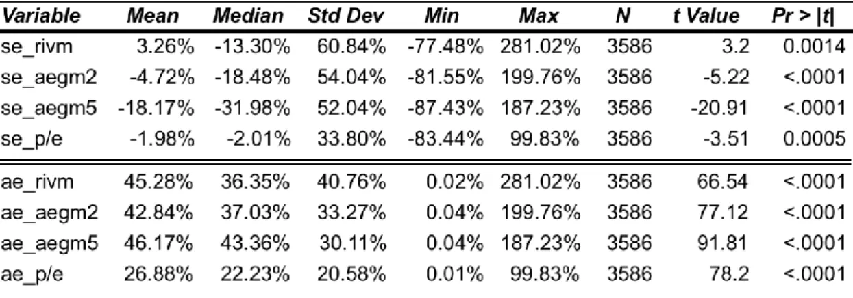
In terms of the entire sample the results are presented in table 3.5. The mean signed error is

negative for all the models, with the exception of RIVM, in which is slightly positive. The

results of RIVM, AEGM2 (AEGM with two-year forecast), AEGM5 (AEGM with five-year

forecast) and P/E are 3.26%, -4.72%, -18.17%,-1.98%, respectively. All the median values

are more negative than mean values. RIVM has -13%, AEGM2 -18%, AEGM5 -32% and P/E

-2%. These results might be a consequence of extreme positive values. Comparing the mean

with median results can be understood that P/E is the only model, which is not affected by

extreme values, since the value of the median is almost equal to mean value. In terms of

absolute errors the extreme values influence is perceptible with lower median values when

comparing to the mean. P/E model is clearly the most accurate model, with practically half of

the value of the other models, in mean and median terms.

These results are in line with the results obtained by Isidro et al. (2006), although the author

just calculates the valuation errors of RIVM and AEGM2. Moreover, a negative signed mean

means that models used underestimate share price, which is the conclusion reached by

Francis et al. (2000).

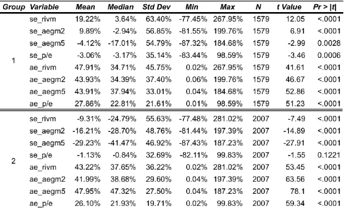
The table 3.6 explores the valuation errors, in signed and absolute terms, for the two groups.

In this table, the difference between mean signed values of each group, are clear. Group 1

shows unrelated figures, for example RIVM 19%, P/E -3%, while group 2 results are all

negative. Analyzing the median values, both groups show a clear negative trend, therefore

underestimating value estimates in relation to share price. In fact, underestimate values

29

model. For example, AEGM5 has a median of -17.01% in group1 and of -41.47% in group 2.

A very careful comparison should be done when comparing absolute mean valuation errors

between both groups. Analyzing separately these figures, one might conclude that valuation

models perform better in the presence of dirty surplus flows, since almost all the models

decrease. In order to confidently reach a conclusion these values should not be analyzed

alone.

I used the median values to cross check the thoughts derived in the previous analysis. In fact,

the median absolute valuation errors increase from group 1 to group 2 in almost all the

models. As stated previously, median valuation is not affected by the extreme values,

moreover, when cross checking the mean values with median values one can understand

that influence in the first measure. Consequently, the increase of median valuation error from

group 1 to group 2 leads to conclude that RIVM, AEGM2 and AEGM5 are affected by the

presence of dirty surplus flows. The valuation models perform worst in the presence of

high-level DSF. The exception is P/E model which decrease the errors from group 1 to group 2.

Furthermore, the median results of RIVM and AEGM2 in group 1 are almost equal, 34.71%

and 34.39% respectively. However, the same measure becomes slightly different in group 2,

37.65% for RIVM and 38.68% for AEGM2. This particular case deserves special attention.

Group 1 results show that in practice RIVM and AEGM 2 have equal values. This is a

consequence of an accounting forecast that respects the CSR, and which is consistent in

terms of growth rate of terminal values, as presented in chapter 2. Therefore one might think

that valuation errors may not be a consequence of dirty surplus flows.

In contrast, the median values of RIVM and AEGM2 are slightly different. In order to

guarantee that the difference is significant, both median of each model were compared for the

different groups, using a median signed paired test. The results are presented in the table

3.7, confirming the insight. While in group 1 the null hypothesis of different median is not

rejected, p-value of 0.9599, the p-value of group 2 is <.0001, rejecting the null hypothesis.

This means that the medians of RIVM and AEGM2 are different in group 2. The main

difference between the two groups is the high level of dirty surplus flows present in group 2.

The previous fact violates one of the assumptions that guarantees the equality between the

two models. So, the presence of dirty surplus flows might be the reason of an increase in

30

The median results of RIVM and AEGM2 are even more controversial. Since AEGM2 has a

slightly higher value than RIVM, 38.68% and 37.65% respectively, mainly due to the

difference of dirty surplus flow levels, it contradicts the previous literature. Academics argued

that AEGM might perform better than RIVM in the presence of DSF, Ohlson (2005) and

Skogsvik and Juettner-Nauroth (2009). The controversial result might be a consequence of

AEGM’s derivation. AEGM formula does not depend on balance sheet statement. Contrarily, RIVM takes in consideration the book value, a balance sheet figure. Although earnings might

be incorrectly forecasted, the balance sheet link might decrease the valuation error.

Another inference that can be done is related with the AEGM5 model. When comparing the

absolute valuation errors of AEGM2 and AEGM5, although their mean is equal in Group1, in

Group 2 the same values already show a considerable difference, 41.99% and 47.95%

respectively. This difference was checked as well. A paired sample t-test concludes that this

difference is not significant in group 1, but it is significant in group 2, as the table 3.8 shows.

More importantly, in terms of median values the difference between both models significantly

increases from Group1 to Group2. In terms of mean difference it was almost 6% while it

increases to almost 10% in terms of median values.

In conclusion, the valuation errors of AEGM model are bigger if the forecast window is bigger.

This effect is stronger in the presence of high level of dirty surplus flows.

Since forecasted earnings might be incorrect due to the presence of dirty surplus, when the

time horizon is extended, then the forecast errors will be bigger as well. Consequently, when

using incorrect earnings and a bigger forecast window, it is expected that valuation errors

become bigger.

P/E model’s results contrast significantly with previous results. This model shows a little improvement from Group1 to Group2 in terms of absolute median valuation errors. These

medians decrease on average from 22.81% to 21.93% and from 27.86% to 26.10%. Although

the results are slightly bigger than the results presented by Liu et al. (2003) they are in line

with them. The difference might be related with the difference of methodologies and with the

influence of the dirty surplus. Overall, the result of P/E model shows its independence from

the dirty’s surplus flows presence, since the change from group 1 to group 2 is insignificant in terms of valuation errors. The independence from dirty surplus flows by P/E model might be

31

I conclude that the P/E valuation model is the most appropriate accounting-based valuation

model to use in the presence of dirty surplus flows, as its accuracy is the best in comparison

to other models. Next comes RIVM, followed by AEGM2 and AEGM5.

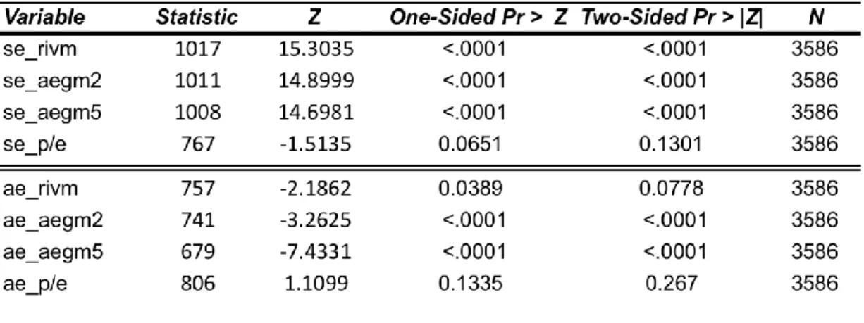
In order to significantly confirm these conclusions, sample t-test, median tests and regression

analysis were executed for each model. The results are shown in table 3.9, 3.10 and 3.11.

The t-test had the objective of confirming the significance of mean differences between the

same models in both groups. To confirm the significance of the median differences a median

two-sample test, summarized in the table 3.10, was used.17 As can be observed in the both

tables, all the models have significant tests in mean and median terms with the exception to

P/E valuation model, which is comprehensible due to P/E model calculation.

Finally, following Francis et al. (2000), a regression analysis was performed with to explain

the valuation estimates in relation with market price. This way individual regressions were

performed for each model, where the actual share price was the dependent variable and the

valuation estimates of each model the independent one. The results, presented in table 3.11,

which follows below, confirm the results obtained with the valuation errors.

Firstly, all regressions are significant, which indicates that the valuation estimates are good

approximations of share price. Secondly, RIVM and both AEGM have a decrease of

explanatory power from group 1 to group 2, for example AEGM2 decreases from an R2 of

57.45% in group1 to an R2 of 46.70% in group 2. This is a consequence of the higher level of

dirty surplus flows which consequently increases the valuation errors and made the value

estimates become less representative of share price. Once again, P/E is the exception,

increasing even the R2 in group 2, from 74.95% to 75.90%, confirming even more its

independence from dirty surplus flows.

VI. Robustness tests

The robustness tests were used to test the sensitivity of the results presented in the previous

section. Robustness tests are related with the main assumptions used to calculate the value

estimates of the accounting models, especially in relation to RIVM and AEGM models and the

17A Wilcoxon two-sample test was also performed for all the models in signed and absolute terms and the results were in line with the ones presented.

32

general conclusion of the results does not change with these tests. The explanation of each

test is detailed below.

Growth rate of Terminal Value

Instead of using the assumed 0.5% as growth rate of terminal value, I used 2.5%. This results

in a general increase of the evaluation errors, which is comprehensible due to its implication

in the value estimates formulas. Even so, the implications drawn from those results are not

significantly different from the ones reached previously.

Cost of Equity Capital

In relation to the cost of equity capital, some modifications were made to the model explained

in appendix 2. Instead of using the firm’s specific beta I used industry-specific ones and instead of using 5% of equity risk premium, 2% and 8% were used. Using the

industry-specific beta the cost of equity capital results are more homogenous with less extremes.

Although the results are more concentrate the inferences that can be made are very similar to

the ones obtained previously. In relation to the change in the equity risk premium, the results

were slightly different from the previous presented, however the extrapolations that can be

33

Table 3.1 – Summary of the Sample Selection Process of Large Sample Analysis

1

X

2

34

Table 3.2 – Summary statistics of primary variables of Large Sample

Table 3.3– Summary statistics of descriptive variables of Large Sample by Group

Table 3.4– Summary statistics of input variables of Large Sample

35

Table 3.6 – Signed and Absolute valuation errors by group

Table 3.7 – Median Signed paired test for RIVM and AEGM2

36

Table 3.9 – Mean sample t-test in signed and absolute terms for all the models

Table 3.10 – Median two-sample test in signed and absolute terms for all the models

Table 3.11 – Regression analysis of value estimates and share price for all the models by group

37

4. Small Sample Analysis - a practical insight on brokers’ reports

I. Introduction

This chapter presents a unique study in terms of dirty surplus flows. This analysis will focus

on the practical use of dirty surplus flows information. In the previous chapter I tested the

performance of different accounting-based valuation models in the presence of dirty surplus

flows. The results show that accounting-based valuations models perform worst in the

presence of high levels of dirty surplus flows, with exception of Multiples.

The previous analysis alerts for the problematic of dirty surplus flows in the valuation process,

however the link with practice is missing. Do brokers consider dirty surplus information in their

reports? If yes, how and where were they usually present? Moreover, which is the most used

valuation model by brokers that considers dirty surplus information?

The small sample analysis allows for a deeper study of this problem, reaching a better

understanding of brokers and how they use the information on dirty surplus. In fact, the

objective is to provide more practical insights into the valuation process of brokers and

complement the conclusions of the large sample.

However, the study of reports, which incorporate dirty surplus information, might shed new

light on the dirty surplus discussion.

With the advantage to study unique and infrequent events that might shed new light on the

dirty surplus problematic, the small sample analysis has as disadvantage the lack of

generalizability of its results.

The results confirm the hypothesis that DSF information is rarely presented in the broker’s reports. When some information about DSF is present in the reports, brokers include it mainly

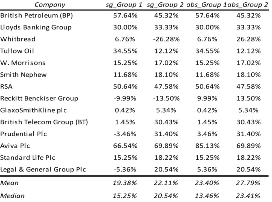
in the valuation model with no explanation or description about it. Moreover, sometimes in

order to understand it, it is necessary to cross check the valuation process with the annual

report of that company.

This chapter is divided in six sections. The first three sections are related with data collection,

period covered and sample selection respectively. The fourth section discusses in detail the

information found in the broker’s reports. Then, I studied the relevance of dirty surplus flows information in the broker’s reports. Finally, the last section presents a case study that deeply