Reversible Current Power Supply for Fast-Field Cycling Nuclear Magnetic Resonance Equipment

Reversible Current Power Supply for Fast-Field Cycling Nuclear Magnetic

Resonance Equipment

M. Lima

, D. M. Sousa

, A. Roque

, E. Margato

DEEC, Instituto Superior Técnico, Universidade de Lisboa

Av. Rovisco Pais, 1 – 1049-001 Lisboa, Portugal

DEEC AC-Energia and INESC-ID, Instituto Superior Técnico, Universidade de Lisboa

Av. Rovisco Pais, 1 – 1049-001 Lisboa, Portugal

,

Escola Superior de Tecnologia de Setúbal/Instituto Politécnico de Setúbal and INESC-ID

Campus do IPS, Estefanilha, 2914-508, Setúbal, Portugal



ADEEEA, ISEL-Instituo Superior de Engenharia de Lisboa, Instituto Politécnico de Lisboa,

and INESC-ID, Av. Rua Conselheiro Emídio Navarro 19059-007 Lisboa,. Portugal

Tel.: +351 – 21 841 74 29.

Fax: +351 – 21 841 71 67.

E-Mail:

[email protected],

[email protected],

[email protected],

[email protected],

URL: http://tecnico.ulisboa.pt, http://www.inesc-id.pt

Acknowledgements

This work was supported by national funds through Instituto Politécnico de Setúbal, for the support to the paper presentation, and FCT – Fundação para a Ciência e a Tecnologia, under project

UID/CEC/50021/2013.

Keywords

«Power Supply», «Fast Field Cycling NMR», «reversible current», «DC/DC converter».

Abstract

The Fast Field-Cycling Nuclear Magnetic Resonance (FFC-NMR) is a technique used to study the molecular dynamics of different types of materials. The main elements of this equipment are a magnet and its power supply. The magnet used as reference in this work is basically a ferromagnetic core with two sets of coils and an air-gap where the materials’ sample is placed. The power supply should supply the magnet being the magnet current controlled in order to perform cycles. One of the technical issues of this type of solution is the compensation of the non-linearities associated to the magnetic characteristic of the magnet and to parasitic magnetic fields. To overcome this problem, this paper describes and discusses a solution for the FFC-NMR power supply based on a four quadrant DC/DC converter.

Introduction

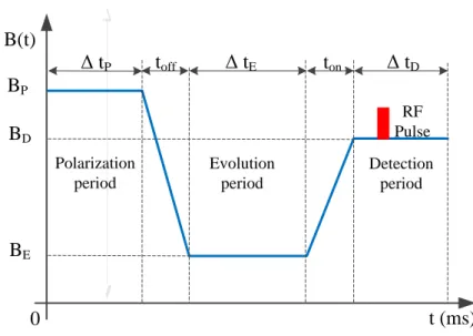
The FFC-NMR is a technique used to measure the spin-lattice relaxation times of different types of materials [1-4]. The FFC-NMR technique is usually implemented by devices having as main elements a magnet and a power supply (Fig. 1) [5-8]. During a FFC-NMR experiment several phases are observed (Fig. 2), during which the samples are submitted to magnetic flux density cycles of different intensity and duration. A regular cycle comprises three phases: the polarization phase, when a

magnetic flux density with high amplitude (BP) is applied in order to magnetize the particles and

arrange them in a certain way. Then, the second step is the evolution phase, where a very low field (BE) is applied during a certain interval, to let the samples rearrange to their equilibrium state, both

magnetically, as well as thermal equilibrium. Finally, there is the detection phase, in which a field of high flux density (BD) is applied preferably during a short period of time.

Sample excitation system (RF Pulse) Power Supply Magnet Software Signal Acquisition System

Probe head and Sample

Coil

Fig. 1: Main blocksof a FFC NMR experiment

B(t) BP BD BE toff ton Δ tP Δ tE Δ tD t (ms) Polarization period Evolution period Detection period RF Pulse 0

Fig. 2: Typical magnetic flux density cycle during a FFC NMR experiment

The main requirements of the power supply are: stability and accuracy values of the magnetic flux density, at each phase of the cycle and the speed on the transitions between the levels of the magnet current [9-11].

The main technical problem of the most recent FFC-NMR relaxometers is to set magnetic flux density levels below 10T. This difficulty is due to the magnetic characteristic of the magnet (hysteresis, saturation and parasitic currents) and due to parasitic magnetic fields, as for instance the components of the Earth magnetic field.

To overcome this technical issue, a new solution for the FFC-NMR power supply, which is new for this type of equipment, is described in this paper. This solution is based on a four quadrant DC/DC converter.

Current source

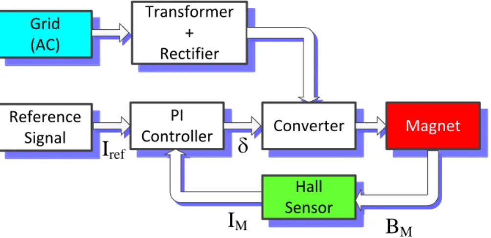
The power supply that drives the FFC magnet current is based on a four quadrant (4Q) DC/DC converter, being the control systems based on a PI controller having as inputs the magnet current

reference signal (Iref) and the actual current of the magnet (IM), which is measured by a Hall Effect

sensor (Fig. 3) [12-15].

Using the 4Q converter is handled the problem associated to non-linearities of the load (hysteresis, saturation and parasitic currents). With this solution, the magnet current range is within the range [-Iα, Imax] in order to set the magnetic flux density within the range [0, Bmax]. With this solution, it is

possible to eliminate the undesirable magnetic field components controlling the magnet current, i.e., magnetizing/demagnetizing the magnet.

Grid (AC) Transformer + Rectifier Reference Signal PI Controller Hall Sensor

I

I

B

d

Fig. 3: Main blocks of the FFC NMR power supply

The topology of the proposed solution is represented in Fig. 4. By setting the switches state it is possible to control the magnet current in order to perform the magnetic flux density cycles, as represented in Fig. 2. The proposed solution is composed by 3 voltage sources (V1, V2 and Vaux), 5

IGBTs (S1, S2, S1aux, S2aux and S3), 4 diodes (D1, D2, D1aux and D2aux), a RC filter (R1; C1) and a boosting

capacitor (Caux; Raux). The FFC magnet has a self-inductance Lm and resistance Rm.

+ -+ - C1 R1 Lm Rm D1 D2 V1 V2 S1 S2 D1aux D2aux S1aux S2aux Caux Raux + -Vaux S3

Fig. 4: Main circuit of the FFC NMR current source

To the proposed solution is possible to identify the following operation modes:

 Steady-state;

 “Up” transition”;

 “Down” transition.

These operation modes are directly related with the states of the semiconductors, and therefore, depend on the voltage source set [16-18]. Voltage sources V1 and V2 assure that the steady-state

currents are within the range [-Iα, Imax]. The voltage source Vaux (Vaux >> V1, V2) is used to speed up the

“Up” transitions.

To explain the power supply operation, it is useful to use the equivalent circuits for each operation mode. For that, the switches can be governed by a set of variables that define their binary state, called state variables, Γ = {γ1, γ2,…, γn}. Being, γi is associated with the state of the semiconductor Si, the

𝛾𝑖= {

0 , 𝑖𝑓 𝑆𝑖 𝑖𝑠 𝑂𝐹𝐹

1 , 𝑖𝑓 𝑆𝑖 𝑖𝑠 𝑂𝑁 ∀ 𝑖 ∈ {1, 2, 3, 1𝑎𝑢𝑥, 2𝑎𝑢𝑥}

(1)

A. Steady-state

The equivalent circuit representing the steady-state operation mode within the current range between 0 and Imax is represented in Fig. 5.

+ -C1 R1 Lm Rm D1 V1 S1 VM IM IC IS1 VC1

Fig. 5: Equivalent circuit for the steady-state operation mode for the range [0, Imax]

In this operation mode, S1 switch alternately, to maintain the magnet current at the desirable level, with

the help of the capacitor C1, which charges and discharges continuously (S3 ON), being the current IS1

provided by voltage source, V1. Being VC1 the voltage of the capacitor C1, the magnet current IM and

the magnet voltage VM are, respectively:

𝐼𝑀= 𝛾1𝐼𝑆1+ (1 − 𝛾1)𝐼𝑐

(2)

𝑉𝑀 ≈ {_𝑉𝑉1, 𝛾1= 1 𝐶1, 𝛾1= 0

(3) When the magnet current is within the range [-Iα, Iα] (low current values), the equivalent circuit is

represented in Fig. 6. + -C1 R1 Lm Rm D1 V1 S1 VM IM IC IS1 VC1 + -D2 V2 S2 IS2

Fig. 6: Equivalent circuit for the steady-state operation mode for the range [-Iα, Iα]

In steady-state, with the magnet current within the range [-Iα, Iα] both semiconductors of the main

converter (S1 and S2) switch alternately, to maintain the current level on the target magnet current.

Again, the capacitor C1 charges and discharges continuously, in order to force a low variation of the

target current value. The capacitor supplies current to the load when S1 is ON and collects current

when S2 is ON.

𝐼𝑀= 𝛾1𝐼𝑆1− 𝛾2𝐼𝑆2+ 𝐼𝑐 (4) 𝑉𝑀 = {_{−𝑈, 𝛾}𝑈, 𝛾1= 1, 𝛾2= 0 1= 0, 𝛾2= 1 (5) Being U=V1=V2. B. “Down” transition

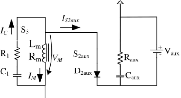
During the “Down” transitions (Fig. 7), S1 and S2 are OFF avoiding interferences with the process of

reducing the magnet current. S3 can be ON during the “down” transition in order to send current back

to the boosting capacitor Caux (S2aux ON). The boosting capacitor shall be bigger than needed, i.e.

should have a higher capacitance value than the value needed for the boost current, so it should be able to take the recharging current from both the magnet and the RC filter.

C1 R1 Lm Rm D2aux S2aux Caux Raux + -Vaux S3 VM IM IS2aux IC

Fig. 7: Equivalent circuit for the “down” transition operation mode The electrical equations for this mode are:

𝐼𝑀+ 𝐼𝑆2𝑎𝑢𝑥 = 𝐼𝑐

(6)

𝑉𝑀 ≈ 𝐼𝑀𝑅𝑚+ 𝐿𝑚𝑑𝐼_𝑑𝑡𝑀

(7) C. “Up” transition

For the “up” transition (Fig. 8), the behavior of the converter is very similar to the “down” transition, but, in this case, it is S1aux that is active. Also, S3 is now OFF, so that, the filter is detached to the rest of

the circuit and the boosting capacitor supply only the load and not the filter’s capacitor.

C1 R1 Lm Rm D1aux S1aux Caux Raux + -Vaux S3 IM

Fig. 8: Equivalent circuit for the “up” transition operation mode The electrical equation for the “up” operation mode is:

𝑉𝑎𝑢𝑥 ≈ 𝐼𝑀𝑅𝑚+ 𝐿𝑚𝑑𝐼_𝑑𝑡𝑀

(8)

Results

To validate the proposed solution, the dynamic behavior of the magnet current is the most important result. For other hand, the power losses constitute a relevant constraint.

A. Power losses

The power losses that need to be studied, for heat dissipation control purposes, are:

- the losses of the semiconductor (diodes and IGBTs): the different types of losses considered are the conduction losses or switching losses, and

- Joule losses.

These power losses depend on a variety of factors and variables such as: the work cycle of the current on the magnet; the duration of the cycle; the filter; the boosting capacitor, Caux; the specifications of

the semiconductors. To calculate the losses, it will be used a non-favorable case scenario, i.e. it will be used the kind of operation that leads to high losses on each of the semiconductors. Considering that the current cycles as the magnetic flux density (Fig. 2), the following values are considered:

 Polarization current: 10 A (0.4T);

 Evolution current: 0 A (0.0T);

 Detection current: 5 A (0.2T);

 I: 2A.

The time duration for each current level are:

 tP: 16 ms  tE: 38 ms  tD: 38 ms  toff: 4 ms  ton: 4 ms  T: 100 ms

For the IGBTs, switching and conduction losses are considered: Conduction losses: 𝑃𝑐_𝑖 = 𝑉_{𝐶𝐸𝑖𝑠𝑎𝑡}𝐼_{𝑆𝑖𝑎𝑣}

(9) Switching losses: 𝑃_𝑆𝑖 = 𝑉_{𝐶𝐸𝑖𝑚𝑎𝑥}𝐼_{𝑆𝑖𝑚𝑎𝑥}(𝑡𝑜𝑛+𝑡𝑜𝑓𝑓

2𝑇 )

(10) Being 𝑉_{𝐶𝐸𝑖𝑠𝑎𝑡} the collector-emitter saturation voltage, 𝐼_{𝑆𝑖𝑎𝑣} is the average IGBT i current, 𝑉_{𝐶𝐸𝑖𝑚𝑎𝑥} is the maximum collector-emitter voltage and 𝐼𝑆𝑖𝑚𝑎𝑥 is the maximum IGBT i current.

For the diodes, only conduction are considered: Conduction losses: 𝑃𝑐𝑖 = 𝑉𝐹𝑖𝐼𝐹𝑖𝑎𝑣

(11) Being 𝑉_𝐹𝑖 the diode i forward voltage and 𝐼_{𝐹𝑖𝑎𝑣} the average current of the diode i.

Besides the losses on the semiconductors it should be taken into account, for the total losses, the Joule losses on the magnet. As it will be observed, these actually represent the major part of the power losses, as there is current flowing in and out of the magnet during most of the period. The equation for the Joule losses is:

𝑃𝑀𝐽 = 𝑅𝑚𝐼𝑀𝑎𝑣

2 ₍₁₂₎

Being 𝐼_𝑀𝑎𝑣 the magnet average current.

For a magnet with Rm = 3Ω, the power losses and the distribution of the power losses are illustrated in

different situations. In fig. 9, are shown the conduction and Joule losses distribution during a typical current cycle.

Fig. 9: Conduction and Joule losses distribution during a current cycle

In Fig. 10 are shown the power losses distribution in the semiconductors for to each operation mode.

Fig. 10: Power losses distribution in the semiconductors according to each operation mode In Fig. 11 are shown the power losses distribution in the magnet for each operation mode.

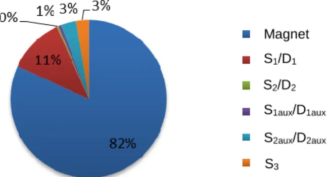
Fig. 11: Power losses distribution in the magnet according to each operation mode In Fig. 12 the total distribution of the power losses during a current cycle.

S1aux/D1aux S2aux/D2aux S3 S2/D2 S1/D1 Magnet “Up” transition Detection level Evolution level Polarization level “Down” transition “Up” transition Detection level Evolution level Polarization level “Down” transition

Fig. 12: Power losses distribution during a current cycle

As expected, the magnet has far superior power loss values, as there is current on it for almost the whole period of operation, unlike the semiconductors. The semiconductors are grouped in pairs Si/Di

because they both conduct at the same time, and both conduction losses are accounted. In the last graph, the losses accounted are in respect to the worst case for each of the semiconductors, and the magnet. It also includes the switching losses of the IGBT, although they represent a very insignificant part of the semiconductors losses, and even less in the total.

B. Magnet current

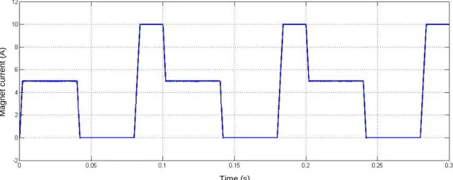
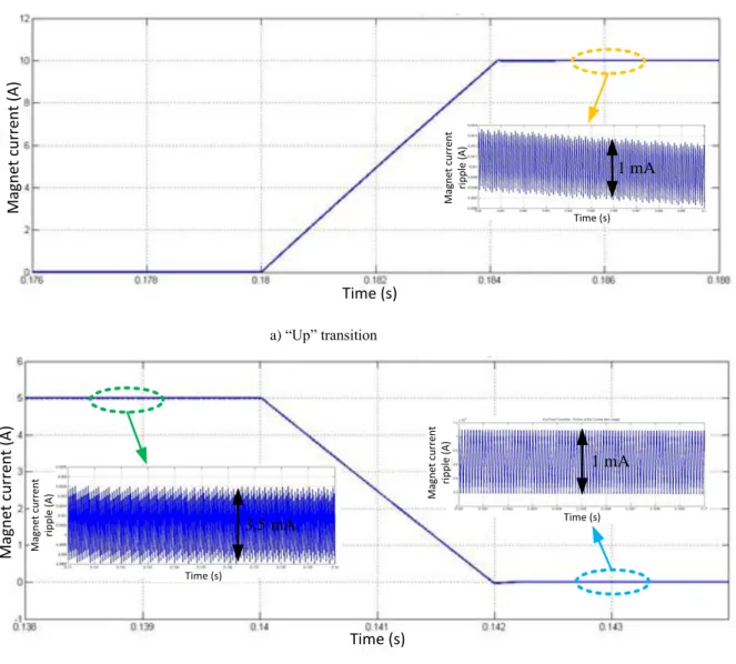
In order to exemplify the performance obtained with the proposed solution, in Fig. 13 is shown the magnet current cycle of a typical FFC-NMR experiment (Current repetitive cycles). In Fig. 14a) is shown the magnet current behavior during an “up” transition and in Fig. 14b), the magnet current behavior during a “down” transition.

It is interesting to observe the speed of the current transitions, i.e., the time required to change from a low current level to a high current level and vice-versa. As it can be seen, the transition rate is 2.5 A/ms, which fulfils the FFC-NMR technique requirements.

Fig. 13: Magnet current cycling

The “up” and “down” current transitions are identical to the other “down” transition, in terms of speed, and stabilization time. In addition, repetitive current cycles are observed, i.e., the magnet current accuracy is also a requirement that should be fulfilled by this solution.

Another important result is the current ripple. The current ripple amplitude and shape, in line with the implemented control method and the parameters set for the controller, can be somehow different according to the current level. For the three current levels used as reference, the maximum current ripple amplitude is about 3.5 mA (zoomed images inside Fig. 14), corresponding to a current variation (of about 0.35%) that does not prevent FFC experiments [19-20].

Joule losses Diodes IGBTs Time (s) M a g n e t c u rr e n t (A )

M ag n et c u rr en t (A ) Time (s) Time (s) M ag n et c u rr en t ri p p le ( A ) 1 mA a) “Up” transition M ag n et c u rr en t (A ) Time (s) Time (s) M ag n et c u rr en t ri p p le ( A ) Mag n et c u rr en t ri p p le ( A ) Time (s) 1 mA 3.5 mA b) “Down” transition

Fig. 14: Magnet current: a) “Up” transition; b) “Down” transition

Conclusion

This paper describes a solution running according the requirements of the FFC-NMR technique, which overcomes technical issues related with parasitic magnetic fields and non-linearities of the magnetic load, since three voltage sources are used in order to control and manage the load current. This paper presents the general aspects related with the operation modes of the proposed circuit and its control system.

About the proposed solution, it is important to point out that are other several aspects that could be discussed about the performance of the proposed solution taking into account the requirements of the FFC NMR technique.

One of the issues not discussed is the semiconductors voltage stress, but the maximum voltages across the semiconductors were taken into consideration, being designed snubbers according to the dynamics required by the application.

As final remark, it should be referred that the magnet was designed in line with the described power supply in order to get a solution fulfilling the FFC NMR requirements.

References

[1] F. Noack, “NMR Field-Cyclying Spectroscopy: Principles and Applications”, Prog. NMR Spectrosc., vol. 18, 1986, pp. 171-276

[2] R. Seitter, R. O. Kimmich, “Magnetic Resonance: Relaxometers”, Encyclopedia of Spectroscopy and Spectrometry, Academic Press, London, 1999, pp. 2000-2008

[3] E. Anoardo, G. Galli, G. Ferrante, “Fast-Field-Cycling NMR: Applications and Instrumentation”, Applied Magnetic

Resonance, vol. 20, 2001, pp. 365-404

[4] R. Kimmich and E. Anoardo, “Field-Cycling NMR relaxometry”, Progress in NMR Spectroscopy, 2004, 44, pp. 257-320 [5] J. Constantin, J. Zajicek, F. Brown, “Fast Field-Cycling Nuclear Magnetic Resonance Spectrometer”, Rev. Sci. Instrum., vol. 67, 1996, pp. 2113-2122

[6] D. M. Sousa, E. Rommel, J. Santana, J. Fernando Silva, P. J. Sebastião, A. C. Ribeiro: Power Supply for a Fast Field Cycling NMR Spectrometer Using IGBTs Operating in the Active Zone, 7th European Conference on Power Electronics and Applications (EPE1997) , Trondheim, Norway, 1997, pp. 2.285-2.290

[7] D. M. Sousa, P. A. L. Fernandes, G. D. Marques, A. C. Ribeiro, P. J. Sebastião: Novel Pulsed Switched Power Supply for a Fast Field Cycling NMR Spectrometer, Solid State Nuclear Magnetic Resonance, vol. 25, 2004, pp. 160-166

[8] D. M. Sousa, G. D. Marques, J. M. Cascais, P. J. Sebastião: Desktop Fast-Field Cycling Nuclear Magnetic Resonance Relaxometer, Solid State Nuclear Magnetic Resonance, vol. 38, 2010, pp. 36-43

[9] A. G. Redfield, W. Fite, H. E. Bleich, “Precision High Speed Current Regulators for Occasionally Switched Inductive Loads”, Review of Scientific Instruments, vol. 39, 1968, pp. 710-715

[10] A. Roque, S. F. Pinto, J. Santana, Duarte M. Sousa, E. Margato, J. Maia: Design of Current Power Sources for a FFC NMR Apparatus: A Comparison, Technological Innovation for Value Creation – DoCEIS 2012, Springer, 2012, pp. 299-308 [11] A.Roque, D. M. Sousa E. Margato, J. Maia: “Current source of a FFC NMR relaxometer linearly controlled”, EPE’13 – 15th European Conference on Power Electronics and Applications, Lille, France, September 2013

[12] Rong-Jong Wai, Yuan Ze, Bo-Han Chen, “High-Efficiency Dual-Input Interleaved DC–DC Converter for Reversible Power Sources”, IEEE Transactions on Power Electronics, 2014, pp. 2903 – 2921

[13] Scortaru, P., Nicolae, D.V. ; Cernat, M. ; Puklus, Z., “Reversible DC-to-DC converter for a dual voltage automotive system using zero voltage switching technique”, 11th International Conference on Optimization of Electrical and Electronic Equipment (OPTIM 2008), 2008, pp. 251 – 258

[14] Yue Wen ; Shao, L. ; Fernandes, R. ; Trescases, O., “Current-mode bi-directional single-inductor three-port DC-DC converter for portable systems with PV power harvesting”, 15th European Conference on Power Electronics and Applications (EPE), 2013

[15] Xuan-Dien Do, Seok-Kyun Han ; Sang-Gug Lee Low power consumption for detecting current zero of synchronous DC-DC buck converter, SoC Design Conference (ISOCC), 2012, pp. 487 – 490

[16] J. F. Silva, S. F. Pinto, Advanced Control of Switching Power Converters, Power Electronics Handbook, Elsevier, 3rd Edition, 2011

[17] J. J. D'Azzo and C. H. Houpis, “Linear Control System Analysis and Design: Conventional and Modern”, 4th Edition, McGraw-Hill, 1995

[18] K. Ogata, “Modern Control Engineering”, 5th Edition, Prentice-Hall, 2010

[19] A. Roque, S. F. Pinto, J. Santana, Duarte M. Sousa, E. Margato, J. Maia, “Dynamic Behavior of Two Power Supplies for FFC NMR Relaxometers”, IEEE International Conference on Industrial Technology – ICIT 2012, Athens - Greece, 2012 [20] D. M. Sousa, G. Marques and P. J. Sebastião: Reducing the size of Fast Field Cycling NMR Spectrometers based on the use of IGBTs, “IEEE ICIT 2009 - International Conference on Industrial Technology”, Churchill - Australia, February 2009