Portfolio rule‐based clustering at automobile insurance in Portugal

                                                           

Portfolio Rule‐based Clustering at Automobile 

Insurance in Portugal 

Octaviani Devi

Internship report presented as partial requirement for 

obtaining the Master’s degree in Statistics and Information 

Management Proposal 

 

 

NOVA Information Management School 

Instituto Superior de Estatística e Gestão de Informação

  Universidade Nova de Lisboa

 

 

PORTFOLIO RULE‐BASED CLUSTERING  

AT AUTOMOBILE INSURANCE IN PORTUGAL 

 

by 

Octaviani Devi 

         

Internship  report  presented  as  partial  requirement  for  obtaining  the  Master’s  degree  in  Advanced  Analytics Proposal.        Advisor / Co Advisor: Roberto Henriques         

 

June 2016 

 

ACKNOWLEDGEMENTS 

 

I wish to express my gratitude to my supervisor, Professor Roberto Henriques, for all his time,  effort, understanding, generous guidance and assistance that made it possible to work in this project.  Also, I would like to extend my gratitude to my supervisors, Paula Santos and Andre Rufino for their  vital comments, supports and valuable discussion. It is a pleasure working with them. I am pleased to  thank  Sjoerd  Smeets for the opportunity and Luis Cardoso who prepare this protocol. Also I would  like  to  thank  the  office  team,  Tiago  Cavaleiro,  Diana  Duarte  and  Filipe  Santos  for  their  help  and  support during the project.  

I  am  pleased  to  thank  Professor  Leonardo  Vanneschi  as  the  head  of  Master  Advanced  Analytics who also support me with his advice. His lectures are amazing. I am also thankful to friends  in Master Advanced Analytics, especially to Thies Bucker, Bruno António, Minang Suh Franklin and Ali  Godjali  for  their  support  and  help.  Also,  I  would  like  to  express  my  gratitude  to  all  my  teachers  in  Master Advanced Analytics.  

Finally,  I  am  thankful  to  my  beloved  friends,  Maria  Tjahjadi  and  Iput  Pudji  Astuti  for  their  endless love, help and care. Also, I dedicate this thesis to my beloved parents and families. 

 

ABSTRACT 

Defining  pricing  strategy  is  a  challenge  for  every  insurance  company.  Competition  makes  insurers  need  to  be  more  careful  to  adjust  the  premium  since  it  may  affect  the  reaction  of  the  existing customer or the new ones. Correspondingly, it may impact the relationship with customer,  also the profitability of the company. Moreover, the increment of number of policies will lead to the  diversity of policy’s risk profile and characteristics which becomes a challenge for insurer to manage  their  portfolio.  Therefore,  a  deep  understanding  of  portfolio  segmentation  is  important  for  the  company to fine tune the pricing strategy and gain more profit. The project aims to discover portfolio  clusters  by  using  k‐means  clustering  algorithm  and  extract  the  rules  of  each  cluster  by  developing  classification  model using  Decision Tree algorithm.  The result of the  model shows that the clusters  give  different  characteristics  and  behavior.  Complement  with  KPI  metrics,  the  company  is  able  to  monitor the  performance of each clusters. So that, the company may use the analyses to optimize  the strategy of growth and profitability. 

Keywords:  automobile  insurance,  rule‐based  clustering,  k‐means,  clustering,  classification,  decision  tree. 

.

CONTENTS 

1.

 

Introduction ... 1

 

1.1.

 

Background and Problem Identification ... 1

 

1.2.

 

Study Objectives ... 2

 

2.

 

Literature Review ... 3

 

2.1.

 

Introduction ... 3

 

2.2.

 

Clustering Based on Rules ... 4

 

2.3.

 

K‐means ... 5

 

2.4.

 

Decision Tree ... 6

 

2.5.

 

Basic Insurance Terms and Ratios ... 6

 

3.

 

Study Relevance and Importance ... 9

 

4.

 

Methodology ... 10

 

4.1.

 

Business Understanding ... 10

 

4.2.

 

Data Understanding and Preparation ... 11

 

4.3.

 

Clustering and Classification Modeling ... 11

 

4.4.

 

KPI Report and Analyses ... 12

 

5.

 

Data Understanding and Preparation Process ... 13

 

5.1.

 

Introduction ... 13

 

5.2.

 

Data Understanding Initialization... 13

 

5.2.1.

 

Variables and Data Sources Identification ... 13

 

5.2.2.

 

Data Dictionary Building ... 15

 

5.3.

 

Source Data Exploration ... 16

 

5.3.1.

 

Source Data Exploration ... 16

 

5.3.2.

 

Data Quality Verification ... 17

 

5.4.

 

Dataset Construction ... 18

 

5.4.1.

 

Dataset Construction ... 18

 

5.4.2.

 

Dataset Exploratory Analysis ... 19

 

5.5.

 

Dataset Preparation ... 20

 

5.5.1.

 

Input Variable Reduction ... 20

 

5.5.2.

 

Dataset Cleaning ... 20

 

5.5.3.

 

Dataset Transformation ... 23

 

6.

 

Modeling ... 24

 

6.1.

 

Modeling Framework ... 24

 

6.2.

 

Cluster Model ... 25

 

6.2.1.

 

Cluster Development Scenario ... 25

 

6.2.2.

 

Selected Meaningful Input Variables ... 26

 

6.2.3.

 

Cluster Model Parameters ... 28

 

6.2.4.

 

Final Cluster Model ... 30

 

6.3.

 

Rule Extraction Model ... 31

 

7.

 

Key Performance Indicator Reports ... 35

 

8.

 

Cluster Characteristic Analyses and Discussion ... 38

 

8.1.

 

Cluster Characteristic Analyses ... 38

 

8.2.

 

Further Characteristics Discussion ... 40

 

9.

 

Summary ... 44

 

9.1.

 

Conclusion ... 44

 

9.2.

 

Limitation and Further Work ... 45

 

10.

 

Bibliography ... 46

 

APPENDIX A. DATASET ... 48

 

APPENDIX B. CLUSTER MODEL ... 51

   

LIST OF FIGURES 

Figure 1: Project Methodologies ... 10

 

Figure 2: Data Understanding and Preparation Process ... 13

 

Figure 3: Model Framework ... 24

 

Figure 4: Cluster Development Scenario ... 25

 

Figure 5 Elbow Method ... 28

 

Figure 6: Proportion of First 12 Cluster Model ... 30

 

Figure 7 Claim Frequency of 12 First Cluster Model ... 31

 

Figure 8: Renewal vs New Business Average Premium ... 41

 

Figure 9: Claim Frequency vs Average Severity ... 41

 

Figure 10: Loss Ratio per Cluster ... 42

 

Figure 11: Loss Ratio vs Claim Frequency ... 42

 

Figure 12: Loss Ratio vs %Growth Policies ... 42

 

LIST OF TABLES 

Table 1: Possible Input Variables ... 15

 

Table 2: Data Source ... 15

 

Table 3: Example of Data Dictionary ... 16

 

Table 4: Data Error Handling ... 18

 

Table 5: Dataset Process Flow ... 18

 

Table 6: Exploratory Analysis ... 19

 

Table 7: Summary Statistics ... 19

 

Table 8: Input Variable Reduction ... 20

 

Table 9: Missing Value Handling Strategies ... 21

 

Table 10: Missing Value Handling ... 21

 

Table 11: Interval Outlier Handling Strategies ... 22

 

Table 12: Nominal Outlier Handling Strategies ... 22

 

Table 13: Interval Outlier Handling ... 23

 

Table 14: Nominal Outlier Handling ... 23

 

Table 15: Selected Input Variables ... 27

 

Table 16: Number of Cluster of Automatic Option ... 29

 

Table 17: First Stage Cluster Model Comparison ... 29

 

Table 18: Second Stage Cluster Model Comparison ... 30

 

Table 19: Final Cluster Model ... 31

 

Table 20: Decision Tree Comparison ... 32

 

Table 21: Interactive Rule Extraction Model ... 33

 

Table 22: Final Ruled‐based Cluster Model... 34

 

Table 23: Key Performance Indicator ... 40

 

LIST OF ABBREVIATIONS AND ACRONYMS 

CBR  Clustering Based on Rules  CCC  Cubic Clustering Criterion  CRISP‐DM  Cross‐Industry Standard Process for Data Mining  GWP  Gross Written Premiums  KPI  Key Performance Indicator  LOB  Line of Business  MAD  Median Absolute Deviation  SSE  Sum of Squared Error  TPL  Third Party Liability

1. INTRODUCTION 

1.1. B

ACKGROUND AND 

P

ROBLEM 

I

DENTIFICATION

 

Once a policy holder is signing the contract and or is renewing it, the insurer is exposed to  the risk. Insurer classifies each risk and calculates the applicable premium associated with that risk.  This  premium  is  the  price  that  a  policy  holder  has  to  pay  for  insurance  coverage.  It  can  vary  significantly  based  on  difference  characteristic  of  the  risk  (Werner  and  Modlin,  2010).  Insurance  premiums  need  to  cover  not  only  the  expected  claims  but  also  certain  level  of  profitability  of  the  company. Therefore, the challenge of pricing strategy is to set premium prices not too high so that  market  share  is  not  impacted  as  customers  have  right  to  exercise  the  price  and  to  choose  their  insurers (Yeo, et all, 2001b).  

Competition is forcing insurers to adjust rates to retain existing customers and to attract new  ones.  Insurance  companies  such  as  automobile  insurances  operate  in  a  more  competitive  environment.  A  policy  holder  easily  switches  from  one  insurer  to  another  because  of  the  price  sensitivity.  The  price  changes  do  not  need  to  be  the  same  across  all  customers.  For  instance,  the  increment by 5% will give different reaction to the policy holder (Guelman, et al, 2014a). Because of  this price change, some policy holders are likely to switch to an alternative insurer, while others will  remain  with  the  same  company.  Insurers  that  implement  pricing  strategy  may  take  benefit  from  customers’ preferences (Dolgui and Proth, 2010). Customers have different purchasing behavior over  time and their willingness to pay. They are attracted by different benefits offered by the same type  of products. For instance, the same car model may be proposed in different versions and may attract  a particular type of customer (Dolgui and Proth, 2010). 

  One of the automobile insurance in Portugal faces the same challenge in defining the pricing  strategy.  The  policy  holders  are  very  sensitive  to  price  changes  as  well  as  claim  management.  In  August 2015, the insurer’s loss ratio is in line with the market which the market’s is 66.8%. However,  this loss ratio is higher about 6.5 pp compare to one of the other insurance company in Portugal. In  addition,  it  is  important  to  the  company  to  manage  cancellation  rate  and  to  see  if  it  is  needed  to  adjust pricing strategy without damaging the relationship with policy holders and to stay competitive  in  the  market.  Customer‐oriented  pricing  can  make  a  significant  contribution  to  performance  enhancement and strengthening the customer relationship (Murdock and McGrail, 1994, cited from  Stomer,  2013).  Stomer  (2013).  It  presents  evidence  regarding  the  importance  of  adjusting  pricing  models by considering consumers’ perception. According to Stomer (2013), in automobile insurance,  vehicle  specific  attributes  are  also  taken  into  consideration  in  premium  calculation  as  well  as  customer  characteristics.  Therefore,  it  is  crucial  to  understand  the  customer  and  vehicle  characteristics. In this case, clustering is used to discover the characteristic similarity by grouping a  heterogeneous population into a number of more homogeneous clusters (Berry and Gordon, 2004).  Furthermore,  rule  extraction  will  be  explored  in  order  to  know  the  characteristics  of  each  cluster.  This project is aligned with the strategic initiative 2015 of the company which is “Capture the non‐life  stand‐alone opportunity in bancassurance” and “Foster Customer Centricity”, also strategic initiative  2020 which are Customer and Innovation. 

1.2. S

TUDY 

O

BJECTIVES

 

From the stated problems, the project aims to discover cluster model that has better split to the  existing  portfolio  in  homogeneous  groups.  The  cluster  model  is  extended  by  building  a  set  of  rules  that extracted from the defined clusters. So that, the rule‐based cluster model is defined and can be  used to assess the pricing strategy. The main objectives of rule‐based cluster model development are  as follow: 

a. Create  portfolio  segments  with  technical  characteristics  such  as  customer  characteristics,  vehicle characteristics or any important characteristics. 

b. Increase  knowledge  of  Motor  portfolios  on  the  technical  Key  Performance  Indicators  (KPIs)  such  as  Loss  Ratio,  Claim  Frequency,  Average  Claim  Cost,  Renewal  Rate  and  Customer  Growth. 

c. Able  to  be  used  to  fine‐tune  motor  pricing  strategy  to  achieve  an  optimized  portfolio  mix  based on discovered cluster model. 

Based on the objectives above, the scope of works of this project is defined. The portfolio data in  this project is limited to the personal portfolio as the majority of the data. Following is the scope of  works:  

a. Identify  variables  used  in  clustering  model  and  identify  parameters  such  as  number  of  clusters. 

b. Develop  portfolio  clusters  of  insurance  portfolios  based  on  their  characteristics  by  using  k‐ means clustering algorithm. Choose the best cluster based on meaningful interpretation and  mathematical decision. 

c. Extract  the  rules  within  the  clusters  by  developing  classification  model.  The  model  is  developed using Decision Tree Algorithm with the respect to the cluster id. 

d. Design and create Key Performance Indicator (KPI) dashboards to enable a better knowledge  of  the  cluster  characteristics.  Provide  analyses  to  understand  the  characteristics  for  each  cluster. 

     

2. LITERATURE REVIEW 

2.1. I

NTRODUCTION

 

Berry and Linoff (2014, p 11, 350) mention that clustering provides a way to learn about the  structure of complex data and break up into similar pieces. In clustering, there are no pre‐classified  classes  and  no  distinction  between  explanatory  and  response  variables.  The  algorithms  discover  similarities  and  group  the  data  into  clusters.  Clustering  methods  have  been  widely  used  in  many  domains,  including  marketing,  pattern  recognition,  biology  and  many  areas.  In  business,  clustering  help  marketer  to  characterize  customer  segmentation  (Brito  et  al,  2015)  and  then  target  the  marketing efforts to the most attractive segment. In biology, it can be used to categorize gene (Hasan  and Duan, 2015) and to derive plant and animal taxonomies (Han and Kamber, 2006). Clustering is  not only used as segmentation but can be used for outlier detection, such as credit card fraud (He,  Xu, Huang & Deng, 2004). However, according to Mirkin (2005), the implementation of clustering is  not  straightforward  because  of  two  factors.  First,  similarity  distance  measurement  and  clustering  techniques frequently give different results. Even though the same technique is implemented, it may  lead  to  different  cluster  solutions  dependent  on  the  choice  of  parameters  such  as  initial  setting  or  number  of  clusters.  Second,  the  interpretation  of  cluster  structures  is  not  straightforward.  In  this  case, the clusters to be found are not depending only to data but also the user’s goal and degree of  granulation.  That  is  why,  clustering  method  often  considered  as  art  rather  than  science.  Although,  Mirkin (2005) mentions that discovered clusters must be treated as an “ideal” representation of the  data that could be used for recovering the original data from aggregate clusters. 

After  in  depth  study  about  available  clustering  techniques  (Han  and  Kamber,  2006),  this  project will focus on partitioning methods. Partitioning methods, k ‐Means, determine the clusters in  such a way that objects within a cluster are “similar”, whereas the objects of different clusters are  “dissimilar”. The clusters have to satisfy the following requirements: (1) each group must contain at  least one object, and (2) each object must belong to exactly one group.  

According to Han and Kamber (2006), one of the most well‐known partitioning methods is k‐ means  algorithm.  The  k‐means  algorithm  takes  the  input  parameter,  k,  and  partitions  a  set  of  n  objects  into  k  clusters  so  that  the  resulting  intra  cluster  similarity  is  high  but  the  inter  cluster  similarity is low. Cluster similarity is measure in regard to the mean value of the objects in cluster.  The algorithm attempts to determine k partitions that minimize the square error function. It works  well  when  the  clusters  are  compact  cloud  separated  from  one  another.  Also,  Han  and  Kamber  say  that  the  method  is  relatively  scalable  and  efficient  in  processing  data  sets.  Correspondingly,  Madhulatha  (2012)  says  the  reason  behind  choosing  the  k‐means  algorithm  is  because  of  its  popularity for the following advantages: (1)  Time complexity of the algorithm is O(nkl), where n is  the  number  of  points,  k  is  the  number  of  cluster,  and  l  is  the  number  of  iterations  taken  by  the  algorithm  to  converge,  it  shows  that  the  k‐means  is  linear  to  number  of  points,  so  that  k‐means  is  scalable and efficient in processing large dataset (2) Space complexity is O(k+n), the space complexity  is  modest  because  only  depend  on  number  of  data  points  and  number  of  clusters  (3)  Order‐ independent,  for  a  given  initial  seed  set  of  clusters,  it  generates  the  same  partition  of  the  data  regardless the order of presented data to the algorithm. A k‐means algorithm often used as customer  segmentation technique among the other clustering techniques (Wang & Keogh, 2008; Liao, Chen &  Lin, 2011; Ghoreyshi, 2015).  

The  major  drawback  of  k‐means  that  mentioned  by  Hand  and  Kamber  is  that  it  often  terminates  at  a  local  optima  and  the  result  largely  depends  on  the  initial  clusters  centers.  Furthermore, the k‐means method can be applied only when the mean of a cluster is defined. This  may  not  be  the  case  in  some  applications,  such  as  when  the  data  have  categorical  attributes.  The  necessity for users to specify k in advance can be seen as a disadvantage. The k‐means method is not  suitable for covering clusters with non‐convex shapes of clusters of very different size. Moreover, it is  sensitive  to  noise  and  outlier  data  points  because  a  small  number  of  such  data  can  substantially  influence the mean value.  

 

2.2. C

LUSTERING 

B

ASED ON 

R

ULES

 

Describing the structure and obtaining the knowledge of a complex system are difficult tasks.  As  mentioned  by  Berry  and  Linoff  (2014),  the  clustering  is  a  way  to  understand  about  it,  however  according  to  Mirkin  (2005),  the  interpretation  of  clusters  is  not  straightforward.  Gibert,  Aluja  and  Cortes (1998) introduce Clustering Based on Rules (CBR) as a methodology that is developed to find  the  structure  of  complex  domains.  This  approach  performs  better  than  traditional  clustering  algorithms  or  knowledge  based  system  approaches.  Gibert,  et  al  explains  that  the  CBR  methods  combine clustering algorithm and inductive learning or supervised learning method that focus to the  problem  of  finding,  interpreting  special  patterns  and  extracting  useful  knowledge.  The  CBR  can  be  seen as a process of building knowledge model of a set of rules.  

Similar  approach  is  introduced  by  Williams  and  Huang  (1997)  which  combine  clustering  method and supervised learning method. The motivation of this approach is driven by the fact that  datasets  become  more  complex  and  extremely  large  nowadays.  The  key  knowledge  or  discoveries  may be lost in this wealth of knowledge clusters and difficult to be analyzed. Therefore, it is needed  to  adopt  a  strategy  to  better  focus  on  the  most  precious  nugget.  In  this  paper,  it  is  presented  hot  spots  methodology  by  adopting  multi  strategies  to  find  the  important  nugget.  Two  cases  are  demonstrated in this study, which are insurance premium setting and fraud detection. The hot spot  methodology has three steps as follows: (1) Develop unsupervised clustering; in this case, k‐means  clustering  algorithm  is  used.  (2)  Perform  supervised  learning  to  build  a  symbolic  description  of  the  clusters. In this project, decision tree is used to produce a rule set. The result of rule is called nugget  which each nugget corresponds to a subset of original dataset. (3) The final step is to evaluate each  nugget in the nugget set to find particular importance based on key variables. Statistical summaries  are  performed  to  evaluate  the  nuggets.  Lastly,  visualization  tools  are  used  to  provide  effective  presentations. 

Moreover,  Han  and  Kamber  (2006)  mention  that  classification  as  supervised  learning  is  an  effective means for distinguish groups or classes of objects. However, it requires labeling and costly  collection to model each group. It is often more desirable to proceed in the reverse direction. First,  separate  the  set  of  data  into  groups  based  on  similarity  by  clustering  and  assign  labels  to  the  relatively small number of groups. Berry and Linoff (2014, p11) also suggest to do clustering as the  first step in a market segmentation effort instead of trying to come up with a one‐size‐fits‐all rule.  Cluster  analysis  can  be  used  as  a  standalone  tool  to  gain  insight  into  the  distribution  of  data,  to  observe  the  characteristics  of  each  cluster,  and  to  focus  on  a  particular  set  of  clusters  for  further  analysis.  A  number  of  studies  have  introduced  clustering  model  as  a  first  step  before  doing 

classification or prediction model. For instance, study from Peng et al (2005) explored unsupervised  learning  method  for  credit  card  accounts  classification.  Jurek  and  Zakrzewska  (2008)  use  cluster  analysis to improve Naïve Bayes Models of Insurance Risk. Lastly, Yeo et al (2001a), use clustering to  classify  policy  holders  into  homogeneous  risk  groups.  Within  each  cluster,  a  prediction  model  is  developed to predict the effect of premium changes on motor insurance. 

Furthermore, data mining technique for application to insurance is introduced by Guo (2003).  Two  important  data  mining  techniques:  cluster  discovery  methods  and  decision  tree  analysis  are  presented  to  address  the  issues  and  techniques  for  casualty  actuaries.  Cluster  analysis  is  implemented  to  discover  groups  and  to  identify  interesting  distributions  and  patterns  in  the  underlying  data,  such  as  segmenting  existing  policy  holders  into  groups  and  associating  a  distinct  profile with each group. This analysis helps insurance company to make rate making strategies and to  select  accurately  which  policies  and  services  to  offer  to  which  customers.  The  example  that  is  showed by Guo is clustering automobile drivers based on geographic and demographic factors. These  segmented drivers will be used to estimate the claim frequency that allows actuaries to evaluate the  potential profit for specific segments. After clustering process, claim frequency model is created by  using combination of decision tree techniques and logistic regression. First, decision tree algorithm is  used  to  identify  the  factors  that  influence  claim  frequency.  After  the  factors  are  identified,  the  logistic  regression  technique  is  used  to  quantify  the  claim  frequency  and  the  effect  of  each  risk  factor.  

Rule‐based  cluster  model  will  be  proposed  in  this  project.  Firstly,  cluster  analysis  will  be  implemented  in  the  interest  of  discovering  the  knowledge  about  insurance  portfolios.  This  knowledge is important for the company to understand portfolio patterns in order to implement the  appropriate strategy for each cluster. A k‐means clustering is used to perform segmentation tasks in  this  study.  It  is  necessary  to  exercise  the  result  of  clustering  to  achieve  a  reliable  and  good  result.  Secondly,  after  getting  the  final  clusters,  further  analysis  of  the  characteristics  of  clusters  are  performed. An empirical tree represents a segmentation of the data is created by applying a series of  simple rules. Decision trees as part of the Induction class of data mining technique will be used in the  respect  of  cluster  id.  Statistical  analysis  and  reports  based  on  key  performance  indicator  will  be  created  to  understand  more  the  characteristics  of  the  clusters.  Finally,  the  analyses  of  the  clusters  will be created.   

2.3. K‐

MEANS

 

The k‐means is clustering algorithm that attempts to divide the entity set in K non‐overlapping  clusters. These clusters are represented by lists of entities and by their centroids. The cluster centroid  is the vectors of means characteristics across the clusters members as a result of iterative procedure.  Formally,  the  cluster  structure  is  represented  by    (subset)  I  and  M‐dimensional,  1, … , .  Subsets   form partition  , … ,   with a set of centroids     , … ,  . 

The clustering process of k‐means is as follows. First, K initial centroids are selected, where K is  pre‐specified  by  the  user  and  indicate  the  desired  number  of  clusters.  The  algorithm  then  selects  cluster centers and each of the observations in the data is assigned to a cluster based on the shortest  distance  of  the  data  point  from  the  cluster  centroid.  New  cluster  centers  are  created  by  averaging 

the  observations  assigned  to  a  cluster.  The  centroid  of  each  cluster  is  then  updated  based  on  the  points assigned to that cluster. This process is repeated until a convergence criterion is satisfied (Wu,  2012).  Suppose  , … ,   is  the  dataset.  The  k‐means  can  be  expressed  by  a  function  that  depends on the proximities of the data points to the cluster centroids as follows: 

min

,   ,  

Where    is  the  weight  of x,    is  the  number  of  data  objects  assigned  to  cluster  ,   ∑  is the centroid of cluster  , K is the number of clusters set by the user and the function  “ ”  computes  the  distance  between  object x  and  centroid  ,  1 .  The  selection  of  the  distance function is based on the squared Euclidean distance, i.e.  . 

 

2.4. D

ECISION 

T

REE

 

Decision tree models are exploratory models that produce a series of decision rules, which can  be expressed in English so they are easy to understand and to interpret by people (Berry and Linoff,  1997).  The  decision  tree  model  is  an  algorithm  that  uses  various  ways  to  split  large  of  data  into  smaller set of records that represents segments with the respect of the target. These segments are  called as node which originates with a root node at the top of the tree that consists of entire data.  The  set  of  rules  that  is  represented  as  a  branch  is  applied  until  the  tree  is  pruned  or  there  is  no  possible  split  and  become  a  leaf  node.  Each  leaf  node  of  the  decision  tree  has  a  group  of  observations as a result of unique rule that can be represented as IF‐THEN logic. The algorithms for  building decision trees uses a sample for the split search by computing the worth and by observing  the  splitting  criteria  such  as  number  of  splits,  level  of  the  tree,  input  variables  type,  and  target  variables  type  (Guo,  2003).  Decision  trees  have  two  techniques  of  splits  into  branches,  which  are  binary splits and multi splits.  

The decision trees are classified into two models based on the target variable type. The model is  called a classification tree, in the case that target variable type is categorical. In the other hand, if the  target  variable  is  continuous,  the  decision  tree  model  is  called  regression  tree.  The  decision  tree  algorithm decides which input variable makes the best split that can separate the records so that a  single class predominates in each group. The measure used to evaluate a potential split is purity. The  purity measures evaluate the splits using gini, entropy, information gain ratio or chi square test for  categorical target variables, while for continuous variable, the algorithm use reduction in variance or  F test. The ability to handle missing value in splitting data becomes one of the advantages of using  decision  tree.  The  effectiveness  of  a  decision  tree  is  determined  by  observing  the  percentage  classified correctly. Decision tree could be combined with the clustering algorithm to find rules and  pattern (Berry and Linoff, 1997). 

2.5. B

ASIC 

I

NSURANCE 

T

ERMS AND 

R

ATIOS

 

As part of the business understanding, it is important to know basic insurance terms and ratios.  Given  that  some  terms  and  ratios  will  be  used  in  this  project  for  example  in  the  input  variables,  analyses and reporting. This section provides some basic concepts of fundamental insurance terms 

and  ratios,  based  on  the  interview  with  Actuary  and  based  on  summary  of  basic  ratemaking  by  Werner  and  Modlin  (2010).  Basically,  insurance  has  two  fundamental  characteristics  according  to  Vaughn (2008), those are shifting risk from individual (called as insured) to another party (called as  insurers) and sharing losses on some equitable basis by substitutes the premium to the uncertainty  loss.  The  process  to  predict  future  losses  and  expenses  becomes  one  of  the  main  activities  in  insurance that is called as ratemaking or insurance pricing. This process will determine the price per  unit of insurance for each exposure unit.  Risk exposure is the basic unit of risk that underlies the insurance premium. The exposure level  is measured in years “insurance”. If the contract is valid for the whole year, then the exposure is 1‐ year insurance. If the insurance only has half year contract (canceled after 6 months or only have 6  months contract) that the insurance will exhibit 0.5 (half year insurance). While pure premium is a  measure of the average loss per exposure of cost per unit of time. This premium must be sufficient to  cover losses and expenses. To obtain the premium, the insurer must predict the claim cost. The pure  premium is calculated as: 

Pure Premium Frequency Severity   Pure Premium N .  C

N .    E     

T .    C

N .  C   

Pure Premium   Tot. cost of Claims Num. of Exposure⁄   

Pure premium shows industry trends in overall loss costs because of the changes in both frequency  and severity. Pure premium only covers cost of claims. The company has expenses for example cost  of  operation  and  maintenance,  cost  reinvestment,  profit  margin,  inflation  and  commissions.  These  expenses  will  be  added  into  pure  premium  and  it  is  called  commercial  premium.  The  difference  between them is usually big. 

  As  can  be  seen  above,  frequency  and  severity  of  loss  is  used  in  determining  the  premium.  Frequency  is  important  feature  of  an  insurance  portfolio.  The  frequency  is  not  the  number  of  accident that occur or number of a contract claim. It is a measure of claims ratio over risk exposure.  Below is the formula: 

Frequency    Num. of Claims Num. of Exposure⁄   

Intuitively, the frequency is zero if number of claims is zero and there is no maximum value of the  frequency. It is useful to compare between portfolios with different characteristics. For example, let  portfolio  A  has  2,000,000  exposures  and  100,000  numbers  of  claims  and  portfolio  B  has  1,000,000  exposures and 100,000 numbers of claims. 

The frequency of Portfolio A 100,000/2,000,000 5%   The frequency of Portfolio B 100,000/1,000,000 10%  

It can be seen that even though the number of claims are the same, the frequencies are different.  Based on example above, it can be said that portfolios B is more likely to have accidents. Analysis of  changes  in  claims  frequency  can  identify  general  industry  trends  associated  with  the  incidence  of  claims  or  the  utilization  of  the  insurance  coverage.  It  can  also  help  measure  the  effectiveness  of  specific underwriting actions. 

  Furthermore, severity or average claim cost is average value of the cost of claims. It is also  called as intensity or severity. For example, in highway, the frequency of accidents is very low but in  general the costs associated with accidents at high speeds are high. In this case, it can be categorized  as high intensity. Analyzing changes in severity provides information about loss trends and highlights  the impact of any changes in claims handling procedures. Below is the formula: 

Severity   Total amount of Claim Costs Num. of Claims⁄   

Claim  cost  itself  is  sum  of  all  costs  associated  with  the  claim  such  as  cost  of  investigation, 

compensation  and  repairs.  In  the  beginning,  claims  are  not  known  by  the  insurer  because  there  is  time lag between initiation of claim process and establishment of final cost. The date when the loss  happens  is  called  accident  date  or  date  of  loss.  Claims  not  currently  known  by  the  insurer  are  referred to as unreported claims or incurred but not reported (IBNR) claims. In this case, the insurer  estimates of the cost of the claim (called reserve) and will be adjusted later. The report date is the  date  when  the  claim  is  known  by  the  insurer  and  is  called  as  a  reported  claim.  Before  the  claim  is  settled,  the  reported  claim  is  considered  as  an  open  claim.  Once  the  claim  is  settled,  this  claim  is  categorized  as  a  closed  claim.  Loss  is  the  amount  of  compensation  paid  under  the  terms  of  the  insurance  policy.  The  difference  between  claim  and  loss  is  term  claim  to  refer  to  the  demand  of  compensation, while loss to refer to the amount of compensation. 

  Lastly, to assess the profitability of the business, the insurers uses loss ratio. Loss Ratio is the  portion of total losses that is paid by each premium dollar. It is calculated as: 

Loss ratio   Pure Premium Average Premium⁄    Loss ratio   Tot. cost of Claims Earned Premium⁄   

,  which  Earned  Premium  is  the  amount  of  the  premium  that  the  insurers  has  already  earned  in  relation  to  the  exposure.  It  can  be  expressed  as  Premium  *  Exposure.  Loss  ratio  is  used  also  to  determine the appropriate pricing and the creation of business strategies. 

3. STUDY RELEVANCE AND IMPORTANCE 

The  insurer  is  the  largest  bancassurance  operator  in  Portugal.  It  offers  a  wide  range  of  life  and  non‐life  insurance.  Currently,  Life  insurance  of  the  Insurer  is  in  the  third,  while  Non‐Life  insurance  is  in  the  sixth  position  in  the  market.  The  automobile  insurance  as  part  of  Non‐Life  insurance  is  in  the  eleventh  position  with  only  2%  of  market  share.  Since  2011,  a  set  of  company  strategies  for  2011  –  2015  has  been  formulated  not  only  to  expand  the  opportunity  and  to  do  penetration in the market but also to focus on maintaining the customers. As automobile insurance  is a very competitive sector in the market, several actions for automobile insurance have been done  to execute the strategies such as creating new product. Additionally, this project becomes the most  recent of strategy execution. 

Several  analyses  have  been  done  using  data  of  August  2015  regarding  to  the  automobile  performances to give insight about the current condition.  The  analyses are done based  on year on  year basis. Total amount  of Gross Written Premiums (GWP) in increases about 13.4% compared to  August 2014 or 1.4% compared to the market growth. This increment expands the market share from  1.8% to 2%. However, total GWP is still below to the company ambition. Also, the cancellation rate  can  be  improved  by  understanding  the  portfolio  characteristics.  Number  of  new  policies  also  increases  about  26.6%  and  number  of  renewal  policies  increases  about  9.3%  compared  to  same  month of the last year. However, the increment of number of polices is followed by the increment of  gross claim for about 25% year on year. Moreover, the gross loss ratio which is proportion of claim  cost  and  premium  is  also  very  high  with  range  between  65%  and  72%  in  2015.  Those  analyses  become the importance of this study. 

Looking at the current condition of automobile figures, one of the initiatives in accord with  company strategic is to understand the portfolio characteristics. For instance, the increment of gross  claims  will  impact  to  the  pricing  strategies  (Werner  &  Modlin,  2010).    While  adjusting  the  pricing  should  be  done  carefully  since  the  reaction  of  each  customer  can  be  different  (Guelman,  et  al,  2014a). A rate increase has a direct impact on the premium customer payment, but there is also an  indirect  impact  as  a  result  of  the  “causal”  effect  of  the  rate  change  on  the  customer’s  decision  to  renew the policy term (Guelman and Guillen, 2014b). As a result, understanding the nature of price  sensitivities at the insurance policy level is valuable for insurers. Moreover, the increment of number  of  policies  will  lead  to  the  diversity  of  policy’s  risk  profile  and  characteristics  which  becomes  a  challenge  for  insurer  to  manage  their  portfolios.  Therefore,  a  deep  understanding  of  portfolio  segmentation is important for the company to maintain the relationships and gain more profit.  

For  this  reason,  in  this  study,  portfolio  data  will  be  explored  by  using  clustering  technique.  The  clustering  algorithm,  k‐means,  will  be  demonstrated  to  get  the  best  clustering  result.  Hence,  insurers can gain insights from the discovered clusters and natural patterns can be revealed (Wang &  Keogh  2008).  For  further  analysis,  will  be  developed  classification  model  using  Decision  Tree  algorithm  in  order  to  build  a  set  of  rules  to  extract  the  knowledge  regarding  to  the  cluster.  KPI  reports will be created to explore further the behavior of the portfolio inside the clusters. 

4. METHODOLOGY 

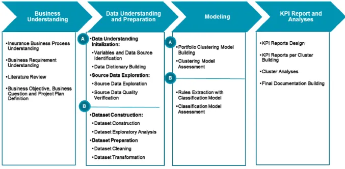
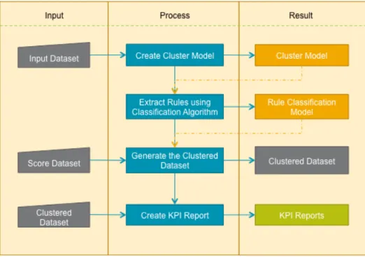
Several  methodologies  are  available  in  data  mining  field.  Azeved  and  Santos  (2008)  do  parallel  comparison between KDD, SEMMA and CRISP‐DM. Based on the study, it is  mentioned that CRISP‐ DM  is  more  complete  methodologies  compared  to  others.  In  CRISP‐DM  methodology,  it  includes  business  understanding  phase  which  is  an  important  phase  in  data  mining  project  while  others  do  not  include  it.  By  understanding  the  problems,  goals  and  resources  in  the  business  understanding  phase, it can minimize the project risk (IBM SPSS Modeler CRISP‐DM Guide, Chapman, 2000).  Some  adjustments are made in the methodology in order to adapt to the project. There are four phases in  the project: (1) Business Understanding, (2) Data Understanding and Data Preparation, (3) Modeling,  and  (4)  KPI  Reports  and  Analyses.  Below  is  the  brief  description  of  the  phases  based  on  IBM  SPSS  Modeler CRISP‐DM Guide and Chapman (2000) with some adaption to the project.  

  Figure 1: Project Methodologies 

4.1. B

USINESS 

U

NDERSTANDING

 

According  to  CRISP‐DM  Guide,  it  is  important  to  explore  what  the  organization  expects  to  accomplish  from  the  data  mining  project.  Therefore,  in  the  initial  phase,  the  first  task  is  to  gain  as  much  insight  as  possible  to  understand  business  objectives  by  clarifying  problems  and  goals  and  discussing with as many key people. However, in order to understand the business requirement, it is  important to know insurance business concept such as business process, insurance terms and ratios.  It  is  useful  not  only  to  understand  the  context  of  the  problem  but  also  to  work  on  data  mining  process.  According  to  Ahlemeyer  and  Coleman  (2014),  the  domain  knowledge  is  a  major  part  of  successful data mining, because taking advantage of the knowledge in data mining decision is done  most of the time, for example in data preparation on how to treat zero and missing values. The next  step  is  assessing  the  situation  regarding  the  available  resources  to  the  project  such  as  business  expert,  data  experts,  dataset  and  software  tools.  Lastly,  converts  the  knowledge  of  business  objectives into data mining goals and preliminary plan designed to achieve the objectives. 

4.2. 0D

ATA 

U

NDERSTANDING AND 

P

REPARATION

 

The  data  understanding  phase  starts  with  data  acquisition  by  performing  any  analysis  and  discussion with business experts. These activities give benefit because specific information regarding  data problem can be provided, so unnecessary process can be avoided (Wang & Keogh, 2008). In this  step, the possible input variables and data sources are identified and collected. Also, data is selected  according  to  the  relevancy  of  data  mining  goal.  The  next  process  is  describing  the  data  including  format,  quantity  and  sampling  of  the  records  by  building  data  dictionary.  In  this  step,  simple  statistical analysis and some graphs or plots are made in order to find some interesting data that may  feed  into  the  transformation  phase.  The  last  step  is  verifying  data  quality  to  discover  of  data  completeness, errors and missing data. 

The  data  preparation  phase  covers  all  activities  to  produce  the  final  dataset  (data  that  will  be  used by modeling). This process normally takes a lot of time and effort in the project. Basic tasks in  data preparation phase are as follows:  

• Data Construction and Integration 

This  task  is  creating  new  data  which  operations  such  as  creating  derived  attributes,  generating records, discretization of data by reducing the number of levels of attribute and  any transforming data activities. There are two basic methods of integrating data which are  merging data set and appending data. Merging data refers to joining together two or more  datasets  that  have  different  information  but  have  the  same  object  information.  In  the  opposite, appending data refers to joining two or more datasets that have same information  but  have  different  object  information.  Deriving  variable  building  and  simplification  of  the  data  such  as  by  aggregating  are  done  in  this  step.  The  result  of  these  processes  is  dataset  that is used by the project. 

• Data Cleaning and Data Transformation 

Data cleaning involves several techniques to solve the data problem such as filling in missing  values,  smoothing  out  noise,  handling  outliers,  detecting  and  removing  redundant  data.  In  this  step,  it  is  possible  to  drop  some  variables.  Last  step  is  data  formatting  which  refer  to  data  transformation.  Sometimes,  certain  modeling  technique  requires  particular  format  or  order to the data.

 

 

 

4.3. C

LUSTERING AND 

C

LASSIFICATION 

M

ODELING

 

In this phase, various modeling techniques are selected and applied. It is possible that this step  has been done in business understanding which refers to the specific modeling technique. Modeling  is usually conducted in multiple iterations because of the needs to fine‐tune the parameters or revert  to  the  data  preparation  phase  for  manipulation  required  by  the  model.  Some  experiment  will  be  done  before  making  final  conclusions.  In  order  to  track  the  progress  with  a  variety  model,  it  is  necessary to keep notes of the parameter setting and data used for each model and description of  model  result.  This  phase  will  be  divided  into  two  which  are  portfolio  clustering  modeling  and  classification modeling based on cluster data. 

4.4. KPI

 

R

EPORT AND 

A

NALYSES

 

At this stage in the project, the data mining models have been built. To understand the result of  clustering  model  in  more  detail,  KPI  reports  will  be  developed.  Further  analyses  per  cluster  will  be  done.  Before  proceeding  to  final  step,  it  is  important  to  more  thoroughly  evaluate  the  model  and  review  the  steps  executed  to  construct  the  model  to  be  certain  it  properly  achieves  the  business  objectives.  A  key  objective  is  to  determine  if  there  is  some  important  business  issue  that  has  not  been  sufficiently  considered.  Final  documentation  is  created  to  record  all  the  activities  and  results  from this project. 

5. DATA UNDERSTANDING AND PREPARATION PROCESS 

5.1. I

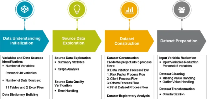
NTRODUCTION

 

Real world data are generally noisy, incomplete and inconsistent that may impact the result of  data mining (Han and Kamber, 2006). Analyzing data that has such problems can produce misleading  or wrong results. Thus, the representation and quality of data is first and foremost before running an  analysis. Data understanding and preparation process will be divided into four groups which are Data  Understanding  Initialization,  Source  Data  Exploration,  Dataset  Construction  and,  lastly,  Dataset  Preparation. The detail of the process is follow: 

  Figure 2: Data Understanding and Preparation Process 

 

5.2. D

ATA 

U

NDERSTANDING 

I

NITIALIZATION

 

The  data  understanding  initialization  is  started  with  the  identification  of  variables  and  data  sources based on Business Understanding phase and Interview with data expert. After the variables  and  data  sources  are  defined,  the  next  step  is  building  data  dictionary  to  document  the  metadata  and to understand the characteristics of the data.  

5.2.1. Variables and Data Sources Identification 

The  main  objective  of  creating  clusters  is  to  determine  pricing  strategies  based  on  the  characteristics of the clusters.  The pricing itself is a function of some observable variables describing  the  risk.  In  motor  vehicle  insurance,  the  pricing  can  be  determined  as  a  function  of  vehicle  characteristics such as power, weight and capacity and customer’s characteristics such as age of the  policy  holder  (

Pelessoni  and  Picech,  1998)

.    Therefore,  the  input  variables  that  are  defined  will  consider risk of portfolio that is used in pricing. The interview with an actuary has been conducted to  decide which variables that possible to be used to create the clustering model.  

There  are  two  types  of  customer  who  buy  insurance  portfolio  which  are  Individual  and  Commercial  Line.  These  customer  types  have  different  data  characteristics.  Thus,  it  is  necessary  to 

split the data into two. The individual data has the majority of the data, in this case, the project only  focus on individual data and filter out the company data. 

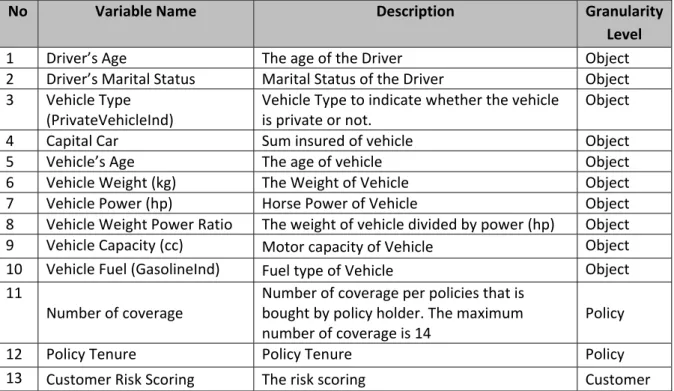
For  the  initial  step,  there  are  39  possible  input  variables  that  has  been  defined  which  are  grouped into five business perspectives. The business perspectives are driver characteristics, vehicle  characteristics,  policy  characteristics,  insurance  customer  characteristics  and  demographic  characteristics. More detail variables are listed below: 

No  Variable Name  Granularity Level 

Driver Characteristics

1  Driver’s Age  Object 

2  Number of Years of Driving License  Object 

3  Driver’s Gender  Object 

4  Driver’s Marital Status  Object 

Vehicle Characteristics

5  Vehicle Type  Object 

6  Capital Car (The current price of the vehicles or sum of insured) Object

7  Vehicle’s Age  Object 

8  Vehicle Weight  Object 

9  Vehicle Power (hp)  Object 

10  Vehicle Weight Power Ratio  Object 

11  Vehicle Capacity (cc)  Object 

12  Vehicle Fuel  Object 

13  Vehicle Brand  Object 

14  Vehicle Number of Seats  Object 

15  Vehicle Number of Doors  Object 

Policy Characteristics

16  Policy Tenure  Policy 

17  Payment Type  Policy 

18  Claim Frequency  Policy 

19  Claim Frequency based on profile  Policy 

20  Average Claim Cost of Contract  Policy 

21  Average Percentage Premium changes at renewal Policy  22  Number of average changes of data  Policy 

23  Number of Coverage  Policy 

24  Collision Coverage Indicator (with or without collision) Policy 

25  Discount per contract  Policy 

Insurance Customer Characteristics

26  Customer Tenure  Customer 

27  Number of Active LOB product Customer 

28  Number of Active Non-Life Ex. Health LOB product of clients Customer 

29  Number of Active Motor policies Customer 

30  Number of Active Life policies Customer 

31  Number of Active Health policies Customer 

32  Number of Active Accident policies Customer  33  Number of Active Multi Risk policies Customer 

34  Customer Risk Scoring  Customer 

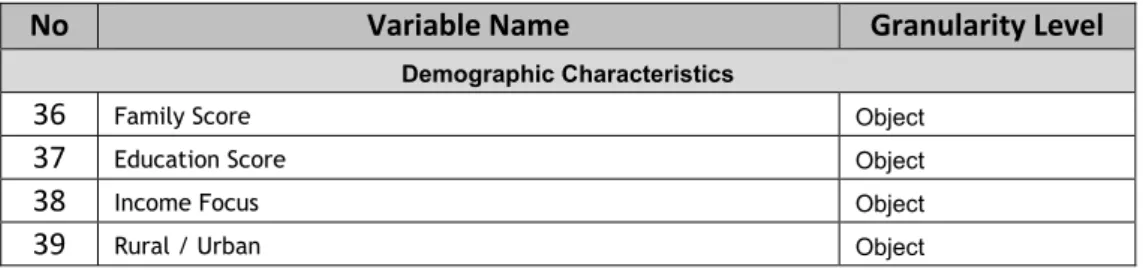
No  Variable Name  Granularity Level 

Demographic Characteristics

36  Family Score  Object 

37  Education Score  Object 

38  Income Focus  Object 

39  Rural / Urban  Object 

Table 1: Possible Input Variables   

After, the possible input variables are identified, the next step is to do the mapping between  input  variables  and  data  source.    The  mapping  document  is  called  as  codebook,  but  it  cannot  be  presented here because of the  confidentiality. In summary, there are 10 tables and 2 excel files of  data sources that will be used in this project, they are:  

No  Source Name  Description 

1  Non‐life Policy Table  This table provides information of all non‐life policies. In this project  this table is used to get the status of policies. 

2  Underwriting Table 

This  table  is  snapshot  values  per  month  based  on  underwriting  point  of  view.  Underwriting  View  shows  the  accumulation  value  annuity.  In  this  view,  the  claim  cost  will  be  reported  on  the  transaction date. This table only contains Motor Policies. 

3  Coverage Table 

This table is information about portfolio per underwriting period. In  this  table,  information  about  coverages  is  used.  This  table  only  contains Motor Policies. 

4  Transaction Table  This is table transaction. This table is used to get number of changes  per policies. 

5  Policy Table  This  is  table  from  Marketing  Data  Mart  that  provides  information  for all policies in the company. 

6  Discount Table  This is table for discount of Motor Policies  7  Risk Score Table  This is table for Risk Score Information 

8  Customer Table  This  is  table  from  Marketing  Data  Mart  that  provides  information  about clients in the company.

9  Demographic Table  This  is  table  from  Marketing  Data  Mart  that  provides  information  about demographics data.  10  Object Table  This is table that contains detail information of objects.  11  Excluded Policies Excel  This is an excel file that contains information of policies that belong  to the company. These policies need to be excluded.  12  Urban Rural Excel  This is an excel file that contains mapping between postal code and  information of Urban, Rural or Mix.  Table 2: Data Source  5.2.2. Data Dictionary Building 

One  of  the  most  valuable  tools  before  performing  data  understanding  is  building  data  dictionary. Data dictionary can give idea about what the data contains. The data dictionary includes  information about data definitions, as follows: 

1. Location of source table  2. The description of the source table  3. Key column(s) of source table  4. Variable Names, Types, Length, English description, example data and some notes.  The full data dictionary document cannot be presented because of the confidentiality. Below is the  example of data dictionary which column ‘Example Data’ uses dummy values:  SAS Folder:  Seguros/Seguros User Data/Marketing/Tabelas  Description:  Table from Marketing Data Mart about all policies Key Column:  Id_Apolice,  ValidoDe 

Name  Type  Label  Description  Example Data 

Cod_Nif  Character  Id Customer     123456789  Id_Apolice  Character  Policy Number     AU12345678  Cod_RamoSimples  Character  LOB 

Line  of  Business  such  as  health, life, and motor. 

AUX‐Protecção  Automóvel  Cod_RamoAgregado  Character  LOB Group     AU‐Automóvel  Dt_EmissaoApolice  Date  Create Date     1/16/13  Dt_InicioApolice  Date  Active Date     1/16/13  Dt_EfeitoAnulacaoApolice  Date  Cancel Date     6/16/15  Nif_EntPagadora  Character  Payer Insurance  Id Customer  Life insurance use this  customer id  123456789  Nif_EntTomadora  Character  Insured Id  Customer  Non‐Life insurance use  this customer id  123456789  ValidoDe  Date  Start Valid Date     8/31/15  ValidoAte  Date  End Valid Date     12/31/99 

Table 3: Example of Data Dictionary 

5.3.

 

S

OURCE 

D

ATA 

E

XPLORATION

 

5.3.1. Source Data Exploration  The second step after data understanding initialization is starting to explore the source data  to get some insights of the data. Following actions are done to analyze the source data:  1. Checking the data integrity  2. Checking key column uniqueness for each table  3. Creating basic information including total records, number of non‐missing value (N), Number  of missing value, Distinct Value  4. Doing univariate analysis, which are divided into two based on the type of variables: 

-

_{Continuous Variables: Summary Statistics / Histogram Chart / Box Plot} 

-

Categorical Variables: One‐way Frequency / Bar Chart / Pie Chart (see the distribution)  The detail data understanding result cannot be presented because of confidentiality. 

5.3.2. Data Quality Verification 

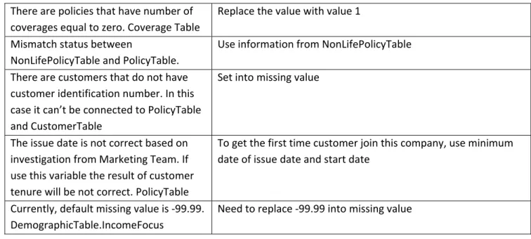
While  doing  exploration  of  source  data,  the  verification  of  data  quality  is  analyzed.  Several  problems such as data error and inconsistencies are found during understanding data process. The  summary of error data handling is follows:  Problem  Explanation and Solution  There are individual ages that higher  than 100.  UnderwritingTable:  - IDD_COND_VALOR  - ANO_CARTA  - CONDSEXO  - CONDESTC     This data means that there is more than 1 driver, so in this case  the ages of the drivers are unknown.  There are rules to change  the  value  into  missing.  This  rule  will  be  applied  for  below  variables for all data:  -  Age  -  Marital Status  -  Gender  - Number of years driving license    The solution is setting variables to missing for all objects that fit  certain rule condition.  There are values of E and T at Marital  Status.  UnderwritingTable.CONDESTC  This is error data. Need to be changed into missing value.  There are values of E and A at Gender.  UnderwritingTable.CONDSEXO  This is error data. Need to be changed into missing value.  There are negative values of total claim  cost. UnderwritingTable (I_FECHADO +  I_CURSO ‐I_IDS_credor)  One of the reasons is because of the rejected claim.  Set to zero for claim cost below than 0  There are zero weight.  UnderwritingTable   ‐ PESOBRUT  In reality, it doesn’t make sense to have zero weight.   In this case, the zero weight values are replaced with the median  weight (exclude zero values) based on cross join between  TP_VIAT (Vehicle Type) and group of VMARCA (Vehicle Brand). It  is applied also for variable WeightPowerRatio.  Zero power of vehicles.  UnderwritingTable   ‐ POTENCIA  Normally zero power is for trailer which is only available at  OTHERS vehicle type. In this case, zero power values are replaced  with median of power based on cross join between TP_VIAT  (Vehicle Type) and group of VMARCA (Vehicle Brand). It is  applied also for variable WeightPowerRatio.  There are differences of Client Type in  same policy but different object.  UnderwritingTable.CLIENT_T  Use the latest CLIENT_T at policy level and use max CLIENT_T at  customer level.  There is difference payment type  between UnderwritingTable. tipfracc and  NonLifePolicyTable. tipfracc  Based on sample policies, the payment type from  UnderwritingTable are correct.  Use information from NonLifePolicyTable  Discrepancy status between  NonLifePolicyTable.sitapol and  UnderwritingTable.  I_CANCELATION_POLICE.  Use information from NonLifePolicyTable. 

There are policies that have number of  coverages equal to zero. Coverage Table  Replace the value with value 1  Mismatch status between  NonLifePolicyTable and PolicyTable.  Use information from NonLifePolicyTable  There are customers that do not have  customer identification number. In this  case it can’t be connected to PolicyTable  and CustomerTable  Set into missing value  The issue date is not correct based on  investigation from Marketing Team. If  use this variable the result of customer  tenure will be not correct. PolicyTable  To get the first time customer join this company, use minimum  date of issue date and start date  Currently, default missing value is ‐99.99.  DemographicTable.IncomeFocus  Need to replace ‐99.99 into missing value    Table 4: Data Error Handling   

5.4. D

ATASET 

C

ONSTRUCTION

 

5.4.1. Dataset Construction 

After  process  of  data  source  exploration  and  data  quality  verification,  the  next  step  is  building  dataset.  In  this  process,  the  cleaner  dataset  can  be  created.  The  dataset  is  built  using  SAS  Enterprise Guide. Based on analysis in the previous step, the project was designed into five process  flows, as follows:   

No  Project Name  Project Description Table Output

0.  Data Initiation  This is used to create active or in‐force policies  that become base dataset for the other process  flows.  CLS_ACTIVE_OBJECTS CLS_ACTIVE_POLICIES  1.  Risk Factor Process Flow  This is used to create variables related to risk  factor  CLS_RISK_FACTOR 

2.  Customer Process Flow  This is used to create variables at customer level CLS_CUSTOMER  3.  Others Process Flow This is used to create other variables  CLS_OTHER  4.  Final Dataset Process  Flow  This is used to create final dataset for individual  after filtering Company Policies  CLS_PERSONAL_DATASET Table 5: Dataset Process Flow 

Table  CLS_PERSONAL_DATASET  is  the  final  dataset  that  is  used  for  modeling.  The  dataset  uses  inforce  policies  of  November  2015  and  consists  about  120,000  records  after  excluding  commercial line data. There are 39 variables that have been developed based on data understanding  initialization  phase.  The  business  rules  and  error  handling  are  also  applied  in  this  dataset.  Detail  process flow diagram from source data into final datasets can be seen at Appendix A.1. 

5.4.2. Dataset Exploratory Analysis 

Dataset  exploratory  analysis  is  also  called  as  descriptive  statistics  normally  based  on  fundamental  statistical  analysis.  The  dataset  is  examined  to  get  prior  information  on  variables  and  their  correlation  before  they  are  selected  as  input  variables  in  the  modeling  process.  The  dataset  exploratory analyses are very useful not only for understanding the variables’ characteristics but also  for giving fundamental statistics information before they are selected for further steps in clustering  analysis. In this project, three analyses have been conducted including univariate analysis, summary  statistics and variable correlations. The analysis is done using SAS Enterprise Guide.  SAS Guide Tools  Description  Characterize Data  To analyze the data including frequency and univariate analysis  Summary Statistics  To analyze the data including basic statistics and percentiles  Correlation  To analyze the correlation between Interval Variables  Table 6: Exploratory Analysis 

  Characterize  data  feature  in  SAS  is  a  simple  approach  to  quickly  getting  a  summary  information of all variables in dataset. In summary, the result of characterize data shows: 

a. Frequency  table  of  categorical  variables.  This  summary  displays  10  most  frequent  distinct  values per variable, frequent count and percent of total frequency. 

b. Descriptive  statistics  of  interval  variables.  This  summary  displays  basic  statistics  such  as  N  (Number  of  non‐missing  values),  NMiss  (Number  of  missing  values),  Total,  Min,  Mean,  Median, Max and StdMean. 

c. Frequency Chart of categorical variables. This chart displays frequent count of each value per  variables in bar chart. 

d. Histogram  Graph  of  interval  variables.  This  graph  displays  frequent  count  of  binning  value  per variables. 

For Summary Statistics, there are 3 categories statistics has been analyzed, those are central  tendency,  dispersion  and  shape  of  distribution.  These  summary  statistics  are  complement  from  previous analysis, which includes shape of distribution such as percentile and skewness.   Category  Common Measures  Central Tendency  Mean and Median  Dispersion  Standard Deviation and Range  Shape of Distribution  Maximum, Minimum, P1, P5, P25, P50, P75, P95, P99, and skewness  Table 7: Summary Statistics 

Correlation  analysis  is  used  to  detect  input  variable  redundancy  in  the  dataset  (Han  and  Kamber,  2004).  The  analysis  uses  correlation  coefficient  (also  known  as  Pearson’s  coefficient)  to  measure  how  strongly  one  attribute  implies  the  other.  However,  the  correlation  does  not  imply  causality. Below are the input variables that are correlated (more than 80%), those are: 

a. Customer Tenure and Policy Tenure have a correlation of 92.3%  b. Driver Age and Years Driving License have a correlation of 83%