Multi-criteria assessment to evaluate potential risk due to exposure to agrochemical products in natura 2000 sites of community importance in Italy

(1)

i

MULTI-CRITERIA ASSESSMENT TO

EVALUATE POTENTIAL RISK DUE TO

EXPOSURE TO AGROCHEMICAL

PRODUCTS IN NATURA 2000 SITES OF

COMMUNITY IMPORTANCE IN ITALY

(2)

ii

NATURA 2000 SITES OF COMMUNITY IMPORTANCE IN ITALY

Dissertation supervised by PhD Pedro da Costa Brito Cabral

Co-supervised by PhD Carlos Granell Canut

PhD Judith Verstegen

(3)

iii

MULTI-CRITERIA ASSESSMENT TO

EVALUATE POTENTIAL RISK DUE TO

EXPOSURE TO AGROCHEMICAL

PRODUCTS IN NATURA 2000 SITES OF

COMMUNITY IMPORTANCE IN ITALY

(4)

iv

NATURA 2000 SITES OF COMMUNITY IMPORTANCE IN ITALY

Dissertation supervised by PhD Pedro da Costa Brito Cabral

Co-supervised by PhD Carlos Granell Canut

PhD Judith Verstegen

(5)

v To Erasmus Mundus program and the European Commission for the sponsorship, making this education possible for me and many other students from all over the world, it was a great honor to be part of this excellent program.

To Professors Marco Painho and Christoph Brox for the coordination of the Master program, to Professor Pedro Cabral for supervising this work, to Professors Judith Verstegen and Carlos Granell Canut for the co-supervision, to Carlo Ciproloni, from ISPRA, for providing the data and for all the clarifications throughout the entire process, to wholly body of teachers and staff from NOVA-IMS, ifgi-WWU and Universitat Jaume I, who have done an excellent job in my academic formation, always with dedication and attention.

To all fellow students who I had the pleasure to share the classroom with. Whether in Portugal, Spain or Germany, you were always whiling to help one another and to exchange a little bit of incredible personal experiences. It was a great opportunity to share different cultures and to make new friendships.

To my wife Priscila for accepting this challenge with me and for the companionship along all this period, to my parents Rita e Fábio, my brother Danilo and his wife Jojô, and all the family who always kept me close even in distant countries.

In memory of Hélio da Rocha Tentilhão.

(6)

vi

MULTI-CRITERIA

ASSESSMENT

TO

EVALUATE

POTENTIAL

RISK

DUE

TO

EXPOSURE

TO

AGROCHEMICAL PRODUCTS IN NATURA 2000 SITES OF

COMMUNITY IMPORTANCE IN ITALY

ABSTRACT

Natura 2000 network is the largest interconnected area of protected sites in the world and covers almost 20% of European Union territory. It entails more than 25.000 sites all over the 27 Member States (Sundseth, 2008). However, many protected areas consist of private lands where agricultural activities have impacts on the conservation of biodiversity and habitats. The spread of large amounts of synthetic agrochemical products, and the consequent contamination of ecosystems, can reduce the biodiversity, triggering selection processes and creating resistant strains to those substances (ISPRA, 2015).

The present work is based on an embraced methodology to evaluate the potential risk from the use of agrochemical products in Natura 2000 Sites of Community Importance (SCI) in Italy. The methodology is founded on a multi-criteria assessment of several variables, combined to generate a simulated risk index. The aim of the project is to develop a replicable geoprocessing workflow to generate the potential Risk Index for SCI in Italy. The use of GIS analysis is addressed to perform an integrated multi-criteria calculation of potential risk, based on the Preliminary Risk Assessment Model for the identification and assessment of problem areas for Soil contamination in Europe (PRA.MS methodology).

The potential Risk Index is an instrument based on a qualitative methodology, constructed from the expert judgment on certain variables. Despite being a qualitative method, the potential Risk Index is an indicator pointing to sites that are potentially in greater danger due to exposure to agrochemicals. Even though there is no “ground-truth” to validate the results, they may serve as a suggestion for further quantitative studies to be carried out in the areas of greatest risk.

(7)

vii

KEYWORDS

Natura 2000

Agrochemical Products Risk Index

Sites of Community Importance Geoprocessing Workflow GIS

(8)

viii

ACRONYMS

CSV – Comma Separated Values EEA – European Environment Agency GI – Geographic Information

GIS – Geographic Information System

ISPRA – Istituto Superiore per la Protezione e la Ricerca Ambientale (Higher Institute

for Protection and Environmental Research)

PRA.MS – Preliminary Risk Assessment Model for the identification, and assessment,

of problem areas for Soil contamination in Europe

SCI – Sites of Community Importance SPA – Special Protection Areas WFS – Web Feature Service

(9)

ix

INDEX OF THE TEXT

Page ACKNOWLEDGMENTS………..v ABSTRACT………..vi KEYWORDS………...vii ACRONYMS………..viii INDEX OF TABLES………..x INDEX OF FIGURES………...xi 1 INTRODUCTION ...1 1.1 Theoretical Framework ………..1

1.2 Aim and Specific Objectives ……..………4

1.3 Assumptions………...6

1.4 General Methodology……….6

1.5 Dissertation Organization………...7

2 PROCEDURES TO CALCULATE THE RISK INDEX………...7

2.1 Chapter objectives ………..7

2.2 Conceptual Model………...7

2.3 Hardware and Software Environment………...10

2.4 Input Dataset………...10

2.5 Geoprocessing Workflow…...13

3 RESULTS………..32

3.1 Risk Map……….…..32

3.2 Histogram and Descriptive Statistics...……….33

3.3 Alternative Classification for Risk Map Visualization…………....………….35

3.4 Scatter Plots……….……….36

3.5 Percentage of Agricultural Land Use in Sites of Community Importance…….37

3.6 Zonal Statistics – Mean Risk Index per Region……….39

4 DISCUSSION AND CONCLUSIONS……….40

BIBLIOGRAPHIC REFERENCES…... 42

APPENDIX...…...44

(10)

x

INDEX OF TABLES

Table 1. Scoring system for percentage of agricultural land use in Sites of Community Importance. Adapted from (ISPRA, 2015)...………... ….…..………… 13

(11)

xi

INDEX OF FIGURES

Figure 1. Overview of Natura 2000 network in Europe ... 1

Figure 2. Natura 2000 Sites of Community Importance and Special Protection Areas in Italy ... 4

Figure 3. Conceptual model for the calculation of potential Risk Index (Adapted from ISPRA, 2015) ... 9

Figure 4. Geoprocessing workflow to calculate the percentage of agricultural land use in Natura 2000 SCI and it respective score (S). ... 14

Figure 5. Geoprocessing workflow to calculate the component Pathway (P) and the respective score for each environmental compartment. ... 19

Figure 6. Geoprocessing workflow to calculate the component Receptor (R) and the respective score for each environmental compartment ... 24

Figure 7. Geoprocessing workflow to calculate the potential Risk Index (RI) for each environmental compartment and the overall final value. ... 28

Figure 8. Risk Index map ... 32

Figure 9. Risk Index histogram and thresholds for risk classes ... 33

Figure 10. Risk Map classified with Natural Breaks (Jenks) ... 35

Figure 11. SCI AREA X RISK INDEX (Quantile classification) ... 36

Figure 12. SCI AREA X RISK INDEX (Natural Breaks classification) ... 36

Figure 13. Percentage of agricultural land use in Natura 2000 SCI in Italy ... 37

Figure 14. Histogram of variable Percentage of Agriculture in SCI. ... 38

(12)

1

1. INTRODUCTION

1.1 Theoretical Framework

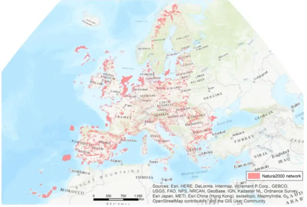
Natura 2000 network is the largest interconnected area of protected sites in the world and covers almost 20% of European Union territory. It entails more than 25.000 sites all over the 27 Member States (Sundseth, 2008). Figure 1 gives an overview of the dimension of Natura 2000 network in Europe.

Figure 1 - overview of Natura 2000 network in Europe. Data source: Natura 2000 (EEA, 2017a)

However, many protected areas consist of private lands where agricultural activities have impacts on the conservation of biodiversity and habitats. The spread of large amounts of synthetic agrochemical products, and the consequent contamination of ecosystems, can reduce the biodiversity, triggering selection processes and creating resistant strains to those substances (ISPRA, 2015).

According to Natura 2000 approach, the protected sites are not “strict nature reserves” and human activities are encouraged to be managed in a sustainable manner, both

(13)

2 ecologically and economically (European Commission, 2017). Nevertheless, the progression towards more intensive land uses and the increasing demand of production leads to agricultural practices that raises concerns about the ecological impacts they can cause. Monocultures that requires heavy application of agrochemicals is the most significant example these agricultural practices.

Concerning this topic, the Directive 2009/128/EC of the European Parliament and the Council of the European Union determines that Member States should implement measures to reduce risks and impacts from the use of pesticides on human health, the environment and biodiversity, in particular on protected areas (Directive 2009/128/EC). This Directive, in Article 12, states the reduction of pesticides and their risks at specific sites: “Member States shall, having due regard for the necessary hygiene and public health requirements and biodiversity, or the results of relevant risk assessments, ensure that the use of pesticides is minimised or prohibited in certain specific areas” (Directive 2009/128/EC).

Nevertheless, when it comes to the use of agrochemicals, it is a complex task to define the source of stressors, how they are dispersed in the environment, which are the exposure pathways, and what are the final receptors or endpoints. Generally, it is not a punctual source of contamination, since the application of agrochemicals is often done by spraying on large parcels of land. Its dispersion in the environment also occurs in different ways in aquatic, terrestrial, or aerial environments. And the final receptors of the contamination chain are essentially dependent on the habitats and species existing over a variety of ecosystems. For that reason, when dealing with the potential risk caused by the exposure of agrochemical substances in the environment, the challenge is the usage of an analysis method capable of covering the multiplicity of sources, exposure pathways and impacted receptors,.

In this sense, literature identifies different approaches for environmental risk assessment depending on the spatial dimension of the problem, two diverse approaches are: site-specific spatial risk assessment and regional risk assessment (Pizzol, 2009). Pizzol discusses the differences between these two approaches and it significances. A site-specific approach is directed to be performed at local scale, where it is possible to spatially identify the source of pollutant (stressor), and often making use of interpolation methods from punctual input data, assisting the allocation of remediation

(14)

3 intervention. Whereas a regional risk assessment deals with larger geographic areas, multiple sources of contamination and stressors, different ecosystems, habitats and diverse spatial relationships between stressors, pathways and receptors. According to Pizzol, the objective of the regional approach is “the prioritization of the risks and the development of a ranking of potentially contaminated sites, in order to identify (…) where preliminary site investigations are required first” (Pizzol, 2009).

To obtain a knowledge base with a regional approach to evaluate how the use of agrochemical products may be affecting Natura 2000 sites in Italy, the Italian Environment Agency (Istituto Superiore per la Protezione e la Ricerca Ambientale - ISPRA - Higher Institute for Protection and Environmental Research) developed a methodology to calculate a potential Risk Index. This method is based on a multi-criteria assessment of several variables, combined to generate a simulated index used to evaluate the potential risk due to the exposure of agrochemical products on protected sites. The term agrochemical products is used here to refer to all types of pesticides, plant protection products, chemical fertilizers or any other phytosanitary product/substance listed on the scope of the project.

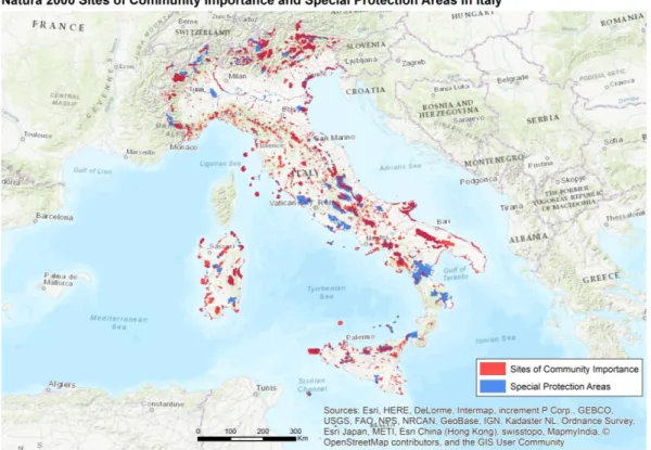
The present project focuses its analysis on the methodology developed to calculate the potential risk index for Sites of Community Importance (SCI), a category of protection in Natura 2000 network. This category of environmental protection is defined on the Habitats Directive of the European Commission. SCI are designated by Members States according to scientific standards and then analyzed by the European Commission before becoming fully part of Natura 2000 network. For more details on the SCI definition criteria, see Habitats Directive (Council Directive 92/43/EEC). Notwithstanding, in some cases there are overlapping areas delimited simultaneously as SCI and Special Protection Areas (SPA) as can be observed in figure 2.

(15)

4

Figure 2 - Natura 2000 Sites of Community Importance and Special Protection Areas in Italy. Data source: Natura 2000 (EEA, 2017b)

The methodology developed by ISPRA provides a different conceptual model and calculation method for the potential risk index on Special Protection Areas (SPA), which is a different category of protection on Natura 2000 network. SPA are defined by the Birds Directive, and it is not part of the scope of the current work. For more details on SPA definition Birds Directive (Directive 2009/147/EC).

1.2 Aim and Specific Objectives

The present work is part of GICases, an initiative co-founded by the Erasmus+ Programme of the European Union, which aims to strengthen relations between the Geographic Information academic field and the industry or public bodies, facilitating collaborative creation, management and sharing of information (GICases, 2017). Consequently, the idea is to bring a real case handled by a governmental agency to the academic field and collaborate with the co-creation and definition of processes, tools and methodologies to enable the sharing of knowledge on a case-based learning practice.

(16)

5 In this context, one of the purposes of this work is to make reproducible the methodology developed by a public agency (ISPRA), bringing it to the academic field in order to exploit it as a form of exercise and interaction between GI studies and problems faced by governments when it comes to planning and managing environmental liabilities.

The aim of this project is to develop a replicable geoprocessing workflow to assess the potential risk due to the exposure to agrochemicals products in Natura 2000 Sites of Community Importance (SCI) in Italy. The use of GIS analysis is addressed to perform an integrated multi-criteria calculation of the potential Risk Index, based on the Preliminary Risk Assessment Model for the identification and assessment of problem areas for Soil contamination in Europe (PRA.MS).

The specifics objectives are:

 to build a model capable of calculate the potential risk index;  represent this spatial information in the format of maps;

 examine the results by the use descriptive statistics and regional analysis.

The purpose of the potential Risk Index to serve as orientation on the definition of measures to reduce the risk related to the use of agrochemicals in areas of environmental protection. From generated results, it is possible identify the sites which are under greater risk and thus establish priority measures of action and control.

The following steps were performed to achieve the specific objectives:  Data acquisition / exploration / format conversion

 Design geoprocessing workflow and Script writing  Production of risk maps

(17)

6

1.3 Assumptions

In the scope of the project it is assumed that the potential Risk Index can be used as an awareness indicative to point the protected sites where the use of agrochemicals has a higher environmental possible damage. Although the index is calculated for discrete surfaces with defined limits, furthermore it assumed that it is possible to make regional analyses with the use of GIS tools, averaging the Risk Index by region with the use of

Zonal Statistics tool.

1.4 General Methodology

The methodology adopted to calculate the potential Risk Index is based on a pre-existing conceptual model developed by the Italian Environmental Agency - ISPRA. The model is established on the methodology PRA.MS, which stands for Preliminary Risk Assessment Model for the identification and assessment of problem areas for Soil contamination in Europe. PRA.MS is one of the results of the project ‘Towards an EEA Europe-wide assessment of areas under risk for soil contamination’. More details about the PRA.MS method can be found on the report published by European Environment Agency (EEA, 2005).

The methodology assumes the paradigm Source-Pathway-Receptor (S-P-R) for the design of the conceptual model. Each one of these components (S-P-R) obtains a score calculated from multiple variables. “PRA.MS adopts a mixed additive and multiplicative algorithm for the calculation of the overall risk index” (ISPRA, 2015). The calculation criteria such as scoring system, weighting factors and the overall risk algorithm are determined based on the judgment of experts about the analysed variables. According to ISPRA, “the lack of established knowledge of the effects of agrochemicals on habitats and species (…) has made it necessary to develop a system based on the knowledge acquired from the scientific literature and on a rational and reproducible approach for the definition of an "expert judgment" (ISPRA, 2015). In this sense, it is a qualitative model where scores are assigned to different variables, based on the judgment of researchers within each specific scientific field.

(18)

7

1.5 Dissertation Organization

The present dissertation is composed of four chapters. The first one is dedicated to the introduction, theoretical framework, aim and objectives, assumptions, and general methodology. The second presents a step-by-step description about the methodology on how to calculate the potential Risk Index. The third chapter is dedicated to the interpretation of results through map visualization and by the use of descriptive statistics. Finally, the fourth and last chapter discusses limitations, considerations and final conclusions.

2. PROCEDURES TO CALCULATE THE RISK INDEX

2.1 Chapter objective

The objective of this chapter is to give a full step-by-step description on how to calculate the potential Risk Index due to exposure to agrochemicals, an explanation about the conceptual model employed in the methodology, followed by hardware and software environment, a description about the input data and how to do the calculations for each part of the model.

2.2 Conceptual Model

As stated previously, the design of the conceptual model is based on the paradigm Source-Pathway-Receptor (S-P-R), where a score is calculated for each one of these components (S-P-R). The scores comes from the results of calculations of multiple variables, depending on the component. In the conceptual model, the characterization for these three components are:

(19)

8  Source (S): represented by the percentage of agricultural land use in Natura

2000 Site of Community Importance;

 Pathway (P): represented by the environmental compartments (surface water, groundwater, soil, air, and food chain), their respective exposure routes (runoff, percolation, volatilization, direct contact) and the chemical-physical properties of pollutant substances. The model make use of solubility, octanol-water

partition coefficient (Kow), persistence or half-life (DT50), steam pressure

(Pv), and aero-dispersion (spray) as chemical-physical variables; and organic

carbon content of the soil (POC), maximum monthly precipitation (Pmax), effective annual mean precipitation (PPeff), aero-dispersion (Spray) as

environmental variables. These properties have been used specifically according to their influence in the prevalent diffusion processes in each environmental sector;

 Receptor (R): represented by the environmental compartments (surface water, groundwater, soil, air, and food chain), eco-toxicological variables corresponding to the target organisms in each compartment (fish, invertebrates,

mammals, birds, bees) and the number of habitats and species in each SCI.

The revision of conceptual model developed by ISPRA is illustrated on Figure 3. It is possible to identify the allocation of variables in relation to the components Source (S), Pathway (P) and Receptor (R) and to the environmental compartments Soil, Water (compartment water is subdivided into groundwater and surface water in component Pathway (P)), Air, and Food Chain.

(20)

9

Figure 3 - Conceptual model for the calculation of potential Risk Index (Adapted from ISPRA, 2015).

For each environmental compartment (soil; water – as a weighted sum between surface and groudwater – air; and food chain) a potential Risk Index (RI) is calculated as the product of the scores of the three components: Source (S), Pathway (P), Receptor (R) and then normalized to 100. For example, the compartment soil is calculated with the following formula:

RI

(soil)

=

(𝑆 ∗

P

(soil)

∗ 𝑅

(soil)

)

10

4

Finally, the overall potential Risk Index (RI) is calculated as the quadratic average of the individual compartments. The final number is expressed in the range 0-100.

RI

=

√

(

RI

(soil)

+RI

(water)+

RI

(air)

+RI

(food-chain)

(21)

10

2.3 Hardware and Software Environment

All the computational procedures were performed in a personal laptop Dell Inspiron 15, processor Intel Core i7, 8GB RAM, 64-bit operating system with Windows 10. Two desktop software were used respectively for calculations and spatial analysis, Microsoft Excel and ArcGIS 10.5.1. The results are published as a Story Map on ArcGIS online and can be view on the following link:



https://risk-index-n2k.maps.arcgis.com/apps/MapSeries/index.html?appid=62913a792b1249a58 7c81bf847e5b931

It was created a personal geodatabase file (extension .mdb) to organize the spatial dataset and the alphanumerical tables, originally obtained from Microsoft Excel files or CSV format. The personal geodatabase file also serves as a workspace, safeguarding the integrity of spatial reference system of the outputs. The Coordinate Reference System utilized for all cartographic layers is WGS 1984 UTM Zone 32N projection Transverse Mercator. Moreover, the personal geodatabase file is also useful to store the ModelBuilder file, which requires an ArcToolBox format to be properly saved. More details about personal geodatabase file can be found at ArcGIS 10.5.1 Help Library (ESRI, 2017).

2.4 Input Dataset

The data used to create and run the model was obtained through different sources. All spatial layers are available online for download in vector format (shapefile). However, there were some difficulties to obtain part of the required data, which was not available online, especially regarding environmental indicators and updated data about the agrochemical substances.

Nevertheless, it was possible to construct a template model combining spatial data obtained through official sources (i.e. EEA and ISPRA online repositories) and data provided by e-mail directly from ISPRA researchers involved in the creation of the model.

(22)

11 The spatial datasets necessary to perform the geoprocessing operations are:

 Natura 2000 Sites of Community Importance: the Italian updated dataset is available for download in shapefile format at EEA repository (EEA, 2017).  Corine Land Cover 2012 level 3: the updated dataset for Italy is available for

download in shapefile format at ISPRA repository (ISPRA, 2017).

 Administrative limits – Italian Provinces: available for download in shapefile format as an INSPIRE dataset in Atom service (GISPORTAL, 2017)

The alphanumeric datasets (originally from Excel files or CSV tables), were obtained separately from the spatial data. This implies on the fact that the tables had to be joined with a spatial layer in order to gather all the data required to calculate the index.

The alphanumeric data provided directly from ISPRA researches are:

 Agrochemical Products Properties: list of the top ten best-selling active substances per Province. It was employed the data regarding the year 2011, as provided on ISPRA report (ISPRA, 2015 – Table 51, Appendix 3). In addition to this list, an excel file containing data for each of the listed substances was provided with respect to the following variables: solubility (S), octanol-water

partition coefficient (Kow), half-life or persistence (DT50), steam pressure (Pv), aero-dispersion (spray). As well as the following eco-toxicological

variables: fish, aquatic invertebrates, algae, mammals, earthworms, birds,

bees, bio-concentration factor (BCF).

 Climatologic data: It was provided as CSV table containing the absolute values for the variables with it respective score already calculated (variables:

maximum monthly precipitation - PPmax, effective annual mean precipitation - PPeff). This table was joined to SCI layer using the site code as primary key.

 Organic carbon content of the soil: It was provided a CSV table containing the SCI code and the score for this variable already calculated for each SCI. This table was joined to SCI layer using the site code as primary key);

(23)

12  Number of habitats and number of species: It was provided an Excel file containing the number of habitats and species for each SIC code. This table was joined to SCI layer using the site code as primary key. The score was calculated afterwards in ArcGIS.

About Agrochemical Products Properties Dataset

For the potential Risk Index calculation, it is considered the ten most sold substances in each province per year. The present project utilizes data regarding the year 2011. It should be noted that there are no data on the sale of agrochemical substances for fifteen Italian provinces: Cagliari, Carbonia-Iglesias, Fermo, Isernia, Matera, Medio Campidano, Monza and della Brianza, Nuoro, Ogliastra, Olbia- Potenza, Rieti, Sassari, Vibo Valentia.

It is assumed that the ten best-selling substances in one province are also the most utilized substances in this same province. Therefore, the scores for each substance is calculated individually according to parameters values. The scores are calculate by macros in Excel worksheet through the creation of conditional clauses (IF ELSE statements).

Afterward, the arithmetic average of the ten substances’ scores is calculated for each province. Therefore the province will have only one row of average scores, instead of ten rows (one per substance). This information is then joined to the province spatial layer, using the Province Code as a primary key.

It is assumed that if one SCI is completely within one province, then this SCI undertakes the scores of that province. Nevertheless, if one SCI is divided into two or more provinces, the weighted average of the scores is calculated according to the percentage of area falling in each province.

It is important to emphasize, in terms of calculation procedures, that the model assumes that every null data, empty row, errors, information not available, etc., gets a value of 0 (zero). It is an arbitrary decision that can affect directly the results. Although this aspect was observed during the elaboration of the present work, the decision was to follow this assumption as recommended by ISPRA researches.

(24)

13

2.5 Geoprocessing Workflow

The geoprocessing workflow was created using ArcGIS ModelBuilder application. More details about the functioning of the ModelBuilder application can be found at ArcGIS Help Library (ESRI, 2017). The process is based on the application of spatial operations between vector layers, spatial join of tables and the calculation of fields based on the formulas presented below. The following sections explain the input data and the steps to calculate each component of the model.

Calculating the score for component SOURCE (S)

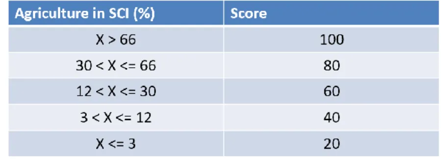
As stated in ISPRA methodology, the score for source of contamination is calculated from percentage of agricultural land use in each SCI. The scores are in the range 0-100 and are established on table 1 (ISPRA, 2015).

Table 1. Scoring system for percentage of agricultural land use in Sites of Community Importance. Adapted from (ISPRA, 2015)

The necessary spatial datasets to perform the calculation are:

 Natura 2000 Sites of Community Importance  Corine Land Cover 2012 – level 3:

(25)

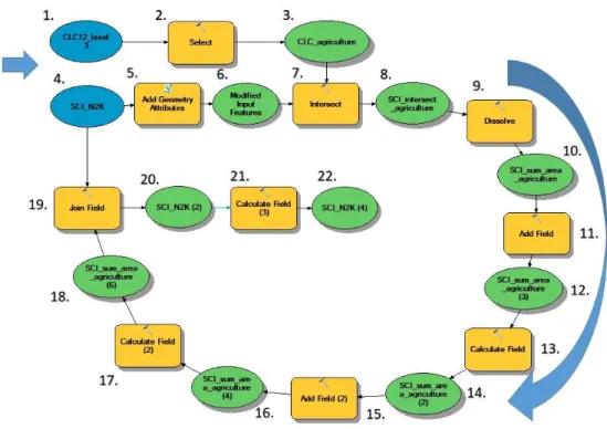
14 The workflow to perform this operation is illustrated on figure 4.

Figure 4 - Geoprocessing workflow to calculate the percentage of agricultural land use in Natura 2000 SCI and it respective score. Blue colour represents input data; yellow colour represents geoprocessing tools; green colour represents the output of each operation.

The input data, geoprocessing tools and outputs are described below. More detailed information regarding the code and logical statements to perform the operations can be found on the Appendix (ArcGIS ModelBuilder Python Script).

1. Input data: spatial layer - Corine Land Cover 2012 level 3 – CLC12_level3 2. Geoprocessing tool: SELECT – It is used to select the classes associated to

agricultural land uses.

3. Output: spatial layer – CLC_agriculture. Selected polygons of agricultural land use.

4. Input data: spatial layer – Natura 2000 Sites of Community Importance -

(26)

15 5. Geoprocessing tool: ADD GEOMETRY ATRIBUTTES – It is used to create a new field on the attribute table and calculate the total area in square meters for each polygon of Natura 2000 SCI.

6. Output: spatial layer – Natura 2000 SCI with an extra field “POLY_AREA” containing the total area of each polygon in square meters.

7. Geoprocessing tool: INTERSECT – It is used to perform the spatial intersection between the layers SCI_N2K and CLC_agriculture.

8. Output: spatial layer – SCI_Intersect_agriculture. It is a layer containing the resultant polygons from the intersection between SCI and agricultural land use. 9. Geoprocessing tool: DISSOLVE – It is used to aggregate the many agricultural

polygons of each individual SCI and sum their area. In this operation, the polygons are merged according to the SCI code and their area is summed. The result is the absolute amount, in square meters, of agricultural land use on each SCI.

10. Output: spatial layer – SCI_sum_area_agriculture. It is a layer containing the absolute amount of agricultural land use in each SCI. The value is expressed in square meters and it is the sum of the area of agricultural polygons belonging to the same SCI.

11. Geoprocessing tool: ADD FIELD – It is utilized to create a new field on the attribute table of the layer SCI_sum_area_agriculture, named

PERCENT_AGRIC. This field is designated to the calculation of the percentage

of agricultural land use in relation to the total area of each SIC.

12. Output: spatial layer – SCI_sum_area_agriculture (3). Attribute table with a new field PERCENT_AGRIC, still with non-calculated values.

13. Geoprocessing tool: CALCULATE FIELD – It is used to calculate the field

PERCENT_AGRIC.

14. Output: spatial layer – SCI_sum_area_agriculture (2). Calculation results for the field PERCENT_AGRIC.

15. Geoprocessing tool: ADD FIELD (2) - It is utilized to create a new field on the attribute table of layer SCI_sum_area_agriculture (2), named SCORE_S. This

(27)

16 field will receive the final values for the score of component Source (S) after calculations.

16. Output: spatial layer – SCI_sum_area_agriculture (4). Attribute table with a new field SCORE_S, still with non-calculated values.

17. Geoprocessing tool: CALCULATE FIELD (2) – It is used to calculate the field

SCORE_S.

18. Output: spatial layer – calculation results for field SCORE_S.

19. Geoprocessing tool: JOIN FIELD – It is employed to join the result fields (PERCENT_AGRIC and SCORE_S) to the attribute table of layer SCI_N2K. 20. Output: spatial layer – SCI_N2K (2). It is equal the original input, plus two new

fields containing the results of the calculation (PERCENT_AGRIC and

SCORE_S).

21. Geoprocessing tool: CALCULATE FIELD (3) – It is applied to calculate the score for the remaining NULL values of the field SCORE_S. The NULL values are due to the fact that are SCIs in which the territory does not intersect with any polygon of agricultural land use. Therefore, there are some SCIs with zero percent of agricultural land within their boundaries. Nevertheless, they receive the minimum score because they present less than 3% of their territory with agricultural land use – as determined on table 1.

22. Output: spatial layer – SCI_N2K (4). It is the final output of this geoprocessing workflow. The result is the SCI layer containing two additional fields on its attribute table. One field “PERCENT_AGRIC” with the percentage of agricultural land use in each SCI; and another “SCORE_S” with the score for the component SOURCE (S) of the potential Risk Index.

Calculating score for component Pathway (P)

The model assumes that the pathways on which agrochemical substances are dispersed in the environment are distributed into environmental compartments. Thus, the pathways are calculated separately, making use of different variables depending on the environmental compartment. The compartments are: a) water (surface/groundwater); b)

(28)

17 soil; c) air; d) food chain. The final score for each compartment ranges between 0-100 and is described as follows:

a.1) Surface water: the calculation is done from the sum of the scores of the variables solubility (wPS), octanol-water partition coefficient (wPKow), half-life (wPDT50), and maximum monthly precipitation (PPmax), related to the evaluation of run-off phenomena, prevalent process associated with surface water (ISPRA, 2015).

Psurface-water = wPs + wPKow + wPDT50 + PPmax

a.2) Groundwater: the calculation is done from the sum of the scores of the same variables, but regarding the climate data it is applied a different variable, effective

annual mean precipitation (PPeff), used in the valuation of infiltration phenomena,

the prevalent process associated with groundwater (ISPRA, 2015).

Pgroundwater = gwPS + gwPKow + gwPDT50 + PPeff

As mentioned before, the final score for component Pathway in water (Pwater) is a weighted sum where surface water represents 80% and groundwater represents 20% of the total value. This decision is based on the assumption that in groundwater the diffusion phenomena is attenuated by the interaction with surface water (ISPRA, 2015).

Pwater = 0,80 * ( Psurface-water) + 0,20 * (Pgroundwater)

b) Soil: the calculation is done from the sum of the scores of the variables

octanol-water partition coefficient (sPKow), half-life (sPDT50) and organic carbon content of the soil (sPOC). Regarding the environmental characteristics, the most significant

variable has been identified as the organic carbon content of the soil, since it is able to increase the natural ability to retain the agrochemical active substance from the soil (ISPRA, 2015).

(29)

18 c) Air: the calculation is done from the sum of the scores of the variables steam

pressure (aPv), and aero-dispersion (aPspray). Agrochemical products reach the air

because they are volatile or as a result of the use in the forma of spray. (ISPRA, 2015).

Pair = aPPv + aPspray

d) Food Chain: the calculation is done from the sum of the scores of the variables

solubility (fcPS), octanol-water partition coefficient (fcPKow), and half-life

(fcPDT50). Agrochemical products reach the "food chain" through accumulation in plants and direct contact with air and soil. These variables determine the persistence in the environment and the bioaccumulation capacity through the food chain. (ISPRA, 2015).

Pfood chain = fcPS + fcPKow + fcPDT50

The necessary spatial datasets to perform the calculation are:

 Natura 2000 Sites of Community Importance – SCI_N2K  Administrative Provinces limits, Italy – Prov2014_WGS84

The required alphanumeric datasets are:

 Agrochemical Products Properties – TOP10_AVERAGE: dataset containing the required chemical-physical variables: solubility (S), octanol-water partition

coefficient (Kow), half-life or persistence (DT50), steam pressure (Pv), aero-dispersion (spray).

 Climatologic information – Rainfall_SIC: dataset containing the following environmental variables: maximum monthly precipitation (PPmax), effective

annual mean precipitation (PPeff) and it respective score already calculated.

 Organic carbon content of the soil – OrganicMatterSIC: dataset containing the SCI code and the score already calculated.

(30)

Figure 5 - Geoprocessing workflow to calculate the component Pathway (P) and the respective score for each environmental compartment. The blue colour represents the input data; yellow colour represents the geoprocessing tools; the green colour represent the output of each operation.

1. Input data: spatial layer – SCI_N2K.

2. Input data: alphanumeric table – Rainfall_SIC. Table containing the climatologic variables (maximum monthly precipitation and efficient

precipitation) and it respective score.

3. Geoprocessing tool: JOIN FIELD (3) – It is employed to join the climatologic variables and it scores to the attribute table of SCI_N2K layer.

4. Output: spatial layer – SCI_N2K (3). Four fields joined to the attribute table (Prec_Max; Sc_PR_Max; Prec_eff; SC_PR_eff).

5. Geoprocessing tool: CALCULATE FIELD (4) – It is applied to calculate the score for NULL values of the field Sc_PR_Max. NULL values are resultant of missing information about the variable maximum monthly precipitation.

(31)

20 Therefore this variable gets value zero (0) for the empty rows and the score is calculated based on this value.

6. Output: spatial layer – SCI_N2K (9). Calculations result for the field

Sc_PR_Max. Eradication of NULL values.

7. Geoprocessing tool: CALCULATE FIELD (5) – It is applied to calculate the score for NULL values of the field Sc_PR_eff. NULL values are resultant of missing information about the variable efficient precipitation. Therefore this variable gets value zero (0) for the empty rows and the score is calculated based on this value.

8. Output: spatial layer – SCI_N2K (5). Calculations result for the field Sc_PR_eff. Eradication of NULL values.

9. Input data: alphanumeric table – OrganicMatterSIC. Table containing the SCI code and it respective score for the variable organic carbon content of the soil. 10. Geoprocessing tool: JOIN FIELD (4) – It is employed to join the field Sc_ORG

to the attribute table of SCI_N2K layer.

11. Output: spatial layer – SCI_N2K (6). Joined field Sc_ORG to the attribute table. 12. Geoprocessing tool: CALCULATE FIELD (6) – It is applied to calculate the

score for NULL values of the field Sc_ORG. NULL values are resultant of missing information about the variable organic carbon content of the soil. Therefore this variable gets value zero (0) for the empty rows and the score is calculated based on this value.

13. Output: spatial layer – SCI_N2K (7). Calculations result for the field Sc_ORG. Eradication of NULL values.

14. Input data: spatial layer – Prov2014_WGS84.

15. Input data: alphanumeric table – TOP10_AVERAGE. Table containing the average scores of the top ten best-selling substances per Province.

16. Geoprocessing tool: JOIN FIELD (5) – It is employed to join the physical-chemical variables average scores to the attribute table of Prov2014_WGS84 layer.

(32)

21 17. Output: spatial layer – Prov2014_WGS84 (3). Physical-chemical score fields

joined to the attribute table.

18. Geoprocessing tool: IDENTITY – It is applied to compute the geometric intersection between the input layer SCI_N2K and the identity layer

Prov2014_WGS84. Therefore, if one SCI is divided into two or more Provinces,

it polygon will be splitted in parts and each part will get the scores corresponding to the Province it belongs to.

19. Output: spatial layer – SCI_identity_Province. It is the resultant layer of IDENTITY operation. The result presents a greater number of polygons than the original SCI_N2K layer because one SCI may be divided into more than one part, according to the number of Provinces it intersects with.

20. Geoprocessing tool: ADD FIELD (5) – It is utilized to create a new field on the attribute table of SCI_identity_Province layer, named P_water. This field will receive the calculation of component Pathway (P) in water.

21. Output: spatial layer – SCI_identity_Province (2). New field P_water added to the attribute table, still with non-calculated values.

P_water.

23. Output: spatial layer – SCI_identity_Province (3). Calculations result for the field P_water.

24. Geoprocessing tool: ADD FIELD (6) – It is utilized to create a new field on the attribute table of SCI_identity_Province layer, named P_soil. This field will receive the calculation of component Pathway (P) in soil.

25. Output: spatial layer – SCI_identity_Province (4). New field P_soil added to the attribute table, still with non-calculated values.

P_soil.

27. Output: spatial layer – SCI_identity_Province (6). Calculations result for the field P_soil.

(33)

22 28. Geoprocessing tool: ADD FIELD (7) – It is utilized to create a new field on the attribute table of SCI_identity_Province layer, named P_air. This field will receive the calculation of component Pathway (P) in air.

29. Output: spatial layer – SCI_identity_Province (5). New field P_air on the attribute table, still with null values.

P_air.

31. Output: spatial layer – SCI_identity_Province (8). Calculations result for the field P_air.

32. Geoprocessing tool: ADD FIELD (8) – It is utilized to create a new field on the attribute table of SCI_identity_Province layer, named P_foodchain. This field will receive the calculation of component Pathway (P) in food chain.

33. Output: spatial layer – SCI_identity_Province (7). New field P_foodchain added to the attribute table, still with non-calculated values.

P_foodchain.

35. Output: spatial layer – SCI_identity_Province (10). Calculations result for the field P_foodchain.

Calculating score for component Receptor (R)

Similarly to the component Pathway (P), the division of the component Receptor (R) into the environmental compartments (water, soil, air, food chain) is required because the scores are associated to different variables, depending on the deliberated target organisms for each environmental compartment. The decision on the variables and species evaluated in the model comes from the judgment of specialists in the specific areas. Further details on the criteria for choosing variables and species can be found in the ISPRA report (ISPRA, 2015). The receptors are considered the endpoint of the contamination chain and in the model they are calculated by sum of the scores from eco-toxicological variables and the number of habitats and species in each SIC.

(34)

23 The final score for each environmental compartment ranges between 0-100 and is described as follows.

 Water: the calculation is done from the sum of the scores of eco-toxicological and site-specific variables, fish (Rfish), aquatic invertebrates (Rinvertebrate), and algae (Ralgae), number of habitats (RnumHab), and number of species (RnumSpe).

Rwater = Rfish + Rinvertebrate + Ralgae + RnumHab + RnumSpe

 Soil: the calculation is done from the sum of the scores of eco-toxicological and site-specific variables, mammals (Rmammals), earthworms (Rearthworms),

number of habitats (RnumHab), and number of species (RnumSpe). Rsoil = Rmammals + Rearthworms + RnumHab + RnumSpe

 Air: the calculation is done from the sum of the scores of eco-toxicological and site-specific variables, birds (Rbirds), bees, (Rbees), number of habitats (RnumHab), and number of species (RnumSpe).

Rair = Rbirds + Rbees + RnumHab + RnumSpe

 Food chain: the calculation is done from the sum of the scores of eco-toxicological and site-specific variables, bio-concentration factor (RBCF),

mammals (Rmammals), birds (Rbirds), fish (Rfish), aquatic invertebrates

(Rinvertebrate), number of habitats (RnumHab), and number of species (RnumSpe).

Rfood chain = RBCF + Rmammals + Rbirds + Rfish + Rinvertebrate + RnumHab + RnumSpe

The necessary spatial datasets to perform the calculation are:  Natura 2000 Sites of Community Importance – SCI_N2K  Administrative Provinces limits, Italy – Prov2014_WGS84

(35)

24 The necessary alphanumeric datasets are:

 Agrochemical Products Properties – TOP10_AVERAGE: dataset containing the required eco-toxicological variables related to target organisms in each environmental compartment: fish (Rfish), aquatic invertebrates (Rinvertebrate), algae (Ralgae), mammals (Rmammals), earthworms (Rearthworms), birds (Rbirds), bees (Rbees).

 Number of Habitats and Number of Species: dataset containing site-specific variables regarding the number of habitats (R_numHAB), and number of species in each SCI (R_numSPE).

The workflow to perform this operation is illustrated on figure 6.

Figure 6 - Geoprocessing workflow to calculate the component Receptor (R) and the respective score for each environmental compartment. Blue colour represents the input data; yellow colour represents the geoprocessing tools; green colour represent the output of each operation. The highlighted part of the model is already computed as part of component Pathway (P), described on Figure 3 (steps 14 to 35).

(36)

25 The input data, geoprocessing tools and outputs are described below. More detailed information regarding the code and logical statements to perform the operations can be found on the Appendix (ArcGIS ModelBuilder Python Script).

1. Input data: spatial layer – SCI_N2K.

2. Input data: alphanumeric table – SIC_N_HAB_SPE. Table containing site-specific variables (number of habitats and number of species) and the SCI code. 3. Geoprocessing tool: JOIN FIELD (2) – It is utilized to join the site-specific

variables to the attribute table of SCI_N2K layer.

4. Output: spatial layer – SCI_N2K (8). Two fields joined to the attribute table (TotaleHAB; TotaleSPE).

5. Geoprocessing tool: ADD FIELD (3) – It is utilized to create a new field on the attribute table of SCI_N2K layer, named R_numHAB. This field will receive the calculation of the score relative to the number of habitats in each SCI.

6. Output: spatial layer – SCI_N2K (10). New field R_numHAB added to the attribute table, still with non-calculated values.

R_numHAB.

9. Geoprocessing tool: ADD FIELD (4) – It is utilized to create a new field on the attribute table of SCI_N2K layer, named R_numSPE. This field will receive the calculation of the score relative to the number of species in each SCI.

10. Output: spatial layer – SCI_N2K (11). New field R_numSPE added to the attribute table, still with non-calculated values.

R_numSPE.

(37)

26 13. Geoprocessing tool: ADD FIELD (9) – It is utilized to create a new field on the attribute table of SCI_identity_Province (9) layer, named R_water. This field will receive the calculation of the score relative to component Receptor (R) in the environmental compartment water.

14. Output: spatial layer – SCI_identity_Province (9). New field R_water added to the attribute table, still with non-calculated values.

R_water.

16. Output: spatial layer – SCI_identity_Province (11). Calculations result for the field R_water.

17. Geoprocessing tool: ADD FIELD (10) – It is utilized to create a new field on the attribute table of SCI_identity_Province (11) layer, named R_soil. This field will receive the calculation of the score relative to component Receptor (R) in the environmental compartment soil.

18. Output: spatial layer – SCI_identity_Province (12). New field R_soil added to the attribute table, still with non-calculated values.

R_soil.

20. Output: spatial layer – SCI_identity_Province (14). Calculations result for the field R_soil.

21. Geoprocessing tool: ADD FIELD (11) – It is utilized to create a new field on the attribute table of SCI_identity_Province (12) layer, named R_air. This field will receive the calculation of the score relative to component Receptor (R) in the environmental compartment air.

22. Output: spatial layer – SCI_identity_Province (13). New field R_air added to the attribute table, still with non-calculated values.

R_air.

24. Output: spatial layer – SCI_identity_Province (16). Calculations result for the field R_air.

(38)

27 25. Geoprocessing tool: ADD FIELD (12) – It is utilized to create a new field on the attribute table of SCI_identity_Province (13) layer, named R_foodchain. This field will receive the calculation of the score relative to component Receptor (R) in the environmental compartment food chain.

26. Output: spatial layer – SCI_identity_Province (15). New field R_foodchain added to the attribute table, still with non-calculated values.

R_foodchain.

28. Output: spatial layer – SCI_identity_Province (18). Calculations result for the field R_foodchain.

Calculating overall potential Risk Index (RI)

After the calculations of components Pathway (P) and Receptor (R) for each environmental compartment (soil, water, air and food chain) a potential Risk Index (RI) is calculated as the product of the scores of the three components: Source (S), Pathways (P), Receptor (R) and then normalized to 100. For example, the compartment soil is calculated with the following formula defined by ISPRA methodology (ISPRA, 2015):

RI

(soil)

=

(𝑆∗

P

(soil)

∗𝑅

(soil)

)

10

4

As a final point, the overall potential Risk Index (RI) is calculated as the quadratic average of the individual compartments. The final number is expressed in the range 0-100 (ISPRA, 2015).

RI

=

√

(

RI

(soil)

+RI

(water)+

RI

(air)

+RI

(food-chain)

(39)

Figure 7 - Geoprocessing workflow to calculate the potential Risk Index (RI) for each environmental compartment and the overall final value. Yellow colour represents the geoprocessing tools; green colour represent the output of each operation. The first input to the model (step 1) is already computed as part of component Receptor (R), described on Figure 4 (last output – step 28).

1. Input data: spatial layer – SCI_identity_Province (18). This layer is the last output (step 28) from the model described on figure 4.

2. Geoprocessing tool: ADD FIELD (13) – It is utilized to create a new field on the attribute table of SCI_identity_Province (18) layer, named RI_water. This field will receive the calculation of the Risk Index (RI) in the environmental compartment water.

3. Output: spatial layer – SCI_identity_Province (17). New field RI_water added to the attribute table, still with non-calculated values.

(40)

29 4. Geoprocessing tool: CALCULATE FIELD (17) – It is used to calculate the field

RI_water.

5. Output: spatial layer – SCI_identity_Province (20). Calculations result for the field RI_water.

6. Geoprocessing tool: ADD FIELD (14) – It is utilized to create a new field on the attribute table of SCI_identity_Province (20) layer, named RI_soil. This field will receive the calculation of the Risk Index (RI) in the environmental compartment soil.

7. Output: spatial layer – SCI_identity_Province (19). New field RI_soil added to the attribute table, still with non-calculated values.

RI_soil.

9. Output: spatial layer – SCI_identity_Province (22). Calculations result for the field RI_soil.

10. Geoprocessing tool: ADD FIELD (15) – It is utilized to create a new field on the attribute table of SCI_identity_Province (22) layer, named RI_air. This field will receive the calculation of the Risk Index (RI) in the environmental compartment air.

11. Output: spatial layer – SCI_identity_Province (21). New field RI_air added to the attribute table, still with non-calculated values.

RI_air.

13. Output: spatial layer – SCI_identity_Province (24). Calculations result for the field RI_air.

14. Geoprocessing tool: ADD FIELD (16) – It is utilized to create a new field on the attribute table of SCI_identity_Province (24) layer, named RI_foodchain. This field will receive the calculation of the Risk Index (RI) in the environmental compartment food chain.

15. Output: spatial layer – SCI_identity_Province (23). New field RI_foodchain added to the attribute table, still with non-calculated values.

(41)

30 16. Geoprocessing tool: CALCULATE FIELD (20) – It is used to calculate the field

RI_foodchain.

17. Output: spatial layer – SCI_identity_Province (26). Calculations result for the field RI_foodchain.

18. Geoprocessing tool: ADD FIELD (17) – It is utilized to create a new field on the attribute table of SCI_identity_Province (26) layer, named RISK_INDEX. This field will receive the calculation of the Risk Index (RI) for each part of the SCI, if it is divided between different Provinces.

19. Output: spatial layer – SCI_identity_Province (25). New field RISK_INDEX added to the attribute table, still with non-calculated values.

RISK_INDEX.

21. Output: spatial layer – SCI_identity_Province (28). Calculations result for the field RISK_INDEX.

22. Geoprocessing tool: ADD FIELD (18) – It is utilized to create a new field on the attribute table of SCI_identity_Province (28) layer, named

PERCENT_AREA. This field will receive the calculation of percentage of area

for each part of the SCI in relation to the total area. Furthermore, this field will be used to calculate the weighted average of the Risk Index (RI).

23. Output: spatial layer – SCI_identity_Province (27). New field

PERCENT_AREA added to the attribute table, still with non-calculated values.

PERCENT_AREA.

25. Output: spatial layer – SCI_identity_Province (30). Calculations result for the field PERCENT_AREA.

26. Geoprocessing tool: ADD FIELD (19) – It is utilized to create a new field on the attribute table of SCI_identity_Province (30) layer, named

RISK_W_AVERAGE. This field will receive the calculation of the weighted

average of the Risk Index. This weighted average is calculated based on the percentage of area that each part represents in relation to the total area of the SCI.

(42)

31 27. Output: spatial layer – SCI_identity_Province (29). New field

RISK_W_AVERAGE added to the attribute table, still with non-calculated

values.

RISK_W_AVERAGE.

29. Output: spatial layer – SCI_identity_Province (32). Calculations result for the field RISK_W_AVERAGE.

30. Geoprocessing tool: DISSOLVE (2) – It is used to aggregate the SCI polygons that were divided into different parts according to the Province. This operation reunify the polygons of the same SCI using the site code as the dissolve field. 31. Output: spatial layer – SCI_dissolve_RI. This is the final output of the model.

In this layer each SCI is represented as a unique row in the attribute table and it has a unique value for the potential risk index, calculated as the weighted average between the parts belonging to the different provinces.

(43)

32

3. RESULTS

The objective of this chapter is to examine the outcomes through the visualization of the results on the format of maps and graphs. Likewise, descriptive statistics and histograms support the understanding of the frequency distribution and the overall resultant values for the Risk Index. Succeeding, an alternative classification method is proposed for result visualization as well as a scatter plot between the sizes of the SCI and the Risk Index. Furthermore, the percentage of agricultural land use in SCI is analysed and finally, it is implemented a regional analysis through the implementation of Zonal Statistics tool.

3.1 Risk Map

Figure 8 represents the final result as a risk map. It is possible to notice the location of the provinces for which there is no available data. As proposed by ISPRA, the Risk Index is a relative measurement where the classes are determined as the division into three homogeneous sets based on the division of three percentiles (Quantiles), each class representing 33,33% of the total amount (ISPRA,2015).

(44)

33

3.2 Histogram and Descriptive Statistics

The histogram with the frequency distribution for the values of the Risk Index is represented on Figure 9. As proposed by ISPRA, the risk classes are determined as the division into three homogeneous classes. The intervals for Risk Index classes are:

 Low: 0 / 7,26

 Medium: 7,27 / 18,69  High: 18,70 / 51,61

Figure 9 - Risk Index histogram and thresholds for risk classes

The analysis of table 2 with the descriptive statistics provides an overall notion about the results:

(45)

34 From the histogram and the descriptive statistics of potential Risk Index, it is possible to affirm:

 The Risk Index was calculated to 2216 Sites of Community Importance (SCI).  It was not possible to calculate the risk for 116 SCI. These SCI are completely contained in Provinces for which there is no data on the sale of agrochemical products. Those 116 SCI do not share their territory with any neighbouring Province.

 Nevertheless, the Risk Index can be calculated for the SCIs that are in one of those “no-data Provinces”, but have part of its territory in another province for which there is available data. In general, the result is very low risk values for the SCIs in this situation. The result is a high frequency of very low values, mainly in coastal SCI, and in those with part of their territory belonging to one of the fifteen provinces for which there is no data on the sale of agrochemicals.  The maximum value is 51,61. It was observed in the SCI named Biviere e

Macconi di Gela, in the south of Sicily.

 The mean value is equal to 14,27 and the standard deviation is equal to 10,17.  The Risk Index is lower than 12,56 in 50 % of cases.

(46)

35

3.3 Alternative Classification for Risk Map Visualization

Figure 10 represents the Risk Index in an alternative perspective, where the symbology is represented in three classes with the classification method Natural Breaks (Jenks), instead of Quantiles. It is possible to notice the difference of the previous classification method on the thresholds for defining the risk classes. When applying Natural Breaks

(Jenks) as the classification method, it is possible to observe that the classes are not

homogenously distributed as in the Quantile method. The resultant classes are represented by 47% of low risk, 33,6 % of medium risk, and 19,4% of high risk.

(47)

36

3.4 Scatter Plots

The graphs were made in order to verify the existence of correlation between the size of the protected sites and the level of risk with the two distinct classification methods, which can be seen respectively on figures 11 and 12. From the analysis of the graphs it is possible to state that there is no direct relationship between the size of the SCI and the Risk Index in both cases.

Figure 11 – SCI AREA X RISK INDEX (Quantile classification). Green colour represents low risk, yellow colour medium risk, and red colour high risk.

Figure 82 – SCI AREA X RISK INDEX (Natural Breaks classification). Green colour represents low risk, yellow colour medium risk, and red colour high risk.

(48)

37 The variation between figures 11 and 12 is the classification method used on the definition of the risk classes low, medium and high. It is possible to observe that the thresholds are not the same, neither is the relative amount of each class in relation to the total: figure 11 presents 33,33% for each class, while figure 12 presents 47% (low risk); 33,6 % (medium risk); and 19,4% (high risk).

3.5 Percentage of agricultural land use in SCI

Figure 13 represents the percentage of agricultural land use in Sites of Community Importance. The symbology is characterized by five classes and the classification method is Natural Breaks (Jenks). The map intends to present a broad panorama, for entire Italy. Nevertheless, the map scale does not favour the visualization of smaller SCI, mainly in the north of the country, in Po river basin and Emilia-Romagna region, which are often characterized by the presence of high proportions of agricultural land use within their boundaries.

(49)

38 Figure 14 shows the frequency distribution of the variable percentage of agriculture in

SCI.

Figure 14 - Histogram of variable Percentage of Agriculture in SCI.

By analysing the histogram it is possible to affirm that:

 The percentage of agricultural land use was calculated to 1863 out of 2332 Sites of Community Importance (SCI). This means that the remaining 469 SCI polygons do not have any spatial intersection with any type of agricultural land use polygon (in Corine land cover classification for the year 2012).

 The maximum value is 100 % of agricultural land use surface. There are 89 protected sites with 100% of their territory occupied only by agriculture.  The mean value is equal to 31,8% and the standard deviation is equal to 32,7.  The percentage of agriculture is lower than 19,4 % in half of the cases.

(50)

39

3.6 Zonal Statistics - Mean Risk Index per Region

To investigate the results with a regional perspective, the resulting vector was converted to raster format in order to implement a zonal statistical analysis. More details about

Zonal Statistics tool can be found on ArcGIS 10.5.1 Help Library (ESRI, 2017). This

tool calculates the mean value of the Risk Index per region. Figure 15 represents the final result as a map.

Figure 15 - Mean Risk Index per Region in Italy.

The regions with the highest mean value are Puglia in the extreme west of the country and Emilia-Romagna in the Po river basin. On the other hand, it should be noted that the regions with the lowest mean values (Sardegna and Basilicata) are those which contain provinces for which there is no data on the sale of agrochemicals. Therefore, this does not necessarily represent that they are under a minor risk, only their Risk Index was not properly calculated due to lack of input data.