Mathematical Modelling of Viscosity Near the Glass Transition: The Random-Walk Approach
Quintas, M.†1, Brandão, T.R.S.†2, Silva, C.L.M. †3, Cunha, R.L. ‡4
†Escola Superior de Biotecnologia, UCP, R. Dr. António Bernardino de Almeida, 4200-072 Porto, Portugal; [email protected]; [email protected]; [email protected].
‡DEA, Faculdade de Engenharia de Alimentos, UNICAMP, Cidade Universitária “Zeferino Vaz”, Caixa Postal 6121, CEP 13081-970, Campinas, SP, Brasil; 4[email protected].
Abstract
The present work deals with the application of the random-walk model, proposed by Arkhipov and Bässler, to describe the viscosity dependence on temperature. Data obtained for sucrose solutions were used to assess the validity of the random-walk approach and the normality of the Density of Possible Metastable States (DPMS). Good results for the fitting of the proposed models were found for fragile liquids. Strong liquids showed poor results and require more investigation.
Key Words: Viscosity, Temperature Dependence, Modelling, Concentrated Solutions, Random-Walk.
Introduction
When a physical phenomenon, usually associated with movement, occurs in a complex way, a random walk can be used to predict the final state of a system. A random-walk is constituted by steps of the same length. At each point, the probability of displacement into another point is independent of the actual position and is equal for all new probable locations.
Arkhipov and Bässler [1] used the random walk approach to develop a model that is able to describe the temperature dependence of viscosity in both strong and fragile liquids [2]. Strong liquids, which usually are tetrahedral network structures, show an Arrhenius dependence of viscosity with temperature and small changes in heat capacity at the glass transition temperature. On the other hand, fragile liquids usually do not present directional bonds and often have ionic or aromatic character. Furthermore, these liquids show strong deviation from Arrhenius behaviour and sharp changes in heat capacity at the glass transition temperature.
The random-walk approach considers two types of excitations in viscous liquids: the elastic, that does not change the system structure neither contributes to viscous flow and loss phenomena; and the inelastic, which is associated with the movement of unit structures in configurational space. Moreover, due to existing strong interactions between structural units, it is not possible for a unit to change its position without the adjacent structures movement and, consequently, a transition in the configurational space occurs. This transition in the configurational space can be considered has a jump of a unit structure in a
highly complex energy landscape. After each jump, the structural unit finds a new environment and the configurational space phase memory is lost. This no memory process can be modelled as a random walk on a disordered network of hopping sites in configurational space, characterised by a broad distribution of energies. Considering that the energy of a structural unit depends on a large number of configurational co-ordinates, each varying randomly, a normalized function can be realistically assumed for the distribution of possible metastable states (DPMS), and the binding energy of a structural unit relatively to the fluid state (E) distribution is given by:
( )
[ ]
(
)
−
−
Γ
=
α
α
− α 0 1 0exp
1
2
)
(
E
E
E
E
E
g
d ; 1 < α < +∞ ; Ed >> E0 (1)where Ed and E0 represent the expected value and the variance of the distribution, respectively, and α a shape parameter of the curve represented by the function. Equation 1 represents a normal distribution when α is equal to 2.
Arkhipov and Bässler [1] considered that only units with energy at or above the expected value for the distribution can execute a movement.
For strong systems, bonds have to be broken in order to allow the movement of a structural unit and the distribution expected value (Ed) is higher than 0. On the other hand, the expected value (Ed) is 0 for fragile liquids, since no energy is required to break bonds. The variance of the DPMS can be comparable for both types of liquids. Considering that for fragile liquids Ed = 0, the normalized function (eq. 1) becomes:
( )
[ ]
−
Γ
=
α
α
− α 0 1 0exp
1
2
)
(
E
E
E
E
g
; 1 < α < +∞ (2)In the case of fragile systems, due to the strong effect of temperature on the energy landscape, two regimes must be considered: i) the lower temperature regime, or supercooled melt “state”, where the density of states function remains static in the time scale of a single jump, and the activation energy of a jump upward in energy is larger than the difference between sites energies; ii) and the higher temperature regime, or real liquid, where the energy landscape is fluctuating at a frequency large enough to allow an unit jump to an adjacent site, and the activation energy of a jump upward in energy is the difference between sites energies.
Considering a random walk, the jump frequency of structural units can be determined using a master equation for the normalized energy distribution function of the structural units [1]. Being the viscosity proportional to the inverse of the jump frequency, and assuming a normal distribution for the DPMS function (α=2), the temperature dependence of viscosity for fragile liquids in the low temperature regime yields:
=
0 2 0exp
2
T
T
η
η
(3)where η0 accounts for the contribution of structural unit jumps towards viscosity and T0 is equal to E0 / kB, being kB the Boltzman constant.
This relation is valid for wide energetic distributions of states (T0 / T >> 1) For the high temperature regime, the relation, valid for T0 / T > 1, becomes:
=
0 0 2 02
exp
2
T
T
T
T
π
η
η
(4)For strong liquids, the viscosity temperature dependence can be described by equation (5), where Td is equal to Ed / kB:
+
=
0 2 0exp
2
T
T
T
T
dη
η
(5)The goal of the present research is to test the applicability of the above-presented models for describing the temperature dependence of viscosity, using sucrose solutions in a wide concentration range (above and below saturation) as model systems. The model was applied to both experimental and published viscosity data of sucrose solutions in a wide range of concentrations. For low concentrations (from 20 to 60% (w/w) in sucrose) data was used from published results [3]. For concentrations above the saturation level, no published data was found and the rheological behaviour was determined experimentally.
Materials and Methods
Solutions with concentrations between 70 and 82.5% (w/w) were prepared by weighing commercial sucrose and adding distilled water to the desired proportion. Then the mixture was heated in a microwave oven for short periods, intercalated with agitation [4, 5] until complete sucrose dissolution. The rheological behaviour of these solutions was studied at temperatures ranging from 0 to 90º C, using a rotational controlled stress rheometer (Carrimed CSL2500, TA Instruments), with 6 cm cone and plate geometry. A creep experiment was used in order to avoid the effects of strong shearing. Creep compliance, under a constant stress of 5 Pa, was measured during the time to reach equilibrium. After the stress was withdrawn, the strain was monitored for a period of time to observe the recovery. This procedure was repeated in triplicate for each sample. Two true replicates of the experiments were also carried out. Non-linear regression analysis, at each experimental sucrose concentration, was performed using the simplex algorithm [6] for function minimization, running in Fortran 77 language.
Results and Discussion
Preliminary results showed a Newtonian behaviour of the concentrated sucrose solutions. Using an ANOVA, no significant difference, at 5% significance, between replicates was found. Concentration and temperature effects on the viscosity were observed.
The temperature dependence of viscosity was studied, by fitting the random-walk model parameters to experimental and published data.
According to the glass transition theory, and assuming the normality of the DPMS function, it is expected that: i) the expression deducted for strong liquids (eq. 5) will describe better the viscosity data of solutions with concentrations below saturation; ii) the expression deducted for fragile liquids in the high temperature regime (eq. 4) should describe the data from concentrations near saturation; iii) and the data obtained at higher concentrations should be better described by the expression deducted to explain the temperature dependence of viscosity of fragile liquids in the low temperature regime (eq. 3).
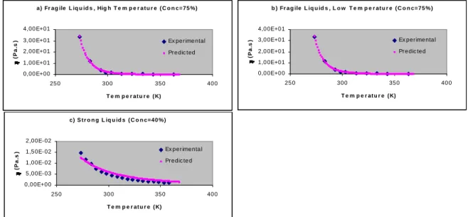
Accordingly, the models were tested in the valid concentration range. A typical fitting, corresponding to each expression deducted, is presented in Figure 1, and the results for the parameters η0, Td and T0 are presented in Table 1. The quality of the regression results for each fitting, including the mean square error (MSE), the adjusted coefficient of determination (R2adj) and the standard half with (in percentage) of the confidence interval at 95% confidence (SHW (%)) are presented in Table 2.
Figure 1. Typical random-walk fitting, using the expressions deducted for strong and fragile liquids in the high and low temperature regimes.
The fitting of the expression (eq. 5), deducted for strong liquids, (Figure 1c) has a minor ability to describe the actual data, compared to the ones deducted for fragile liquids (Figures 1a and b). Although the MSE and R2adj present good values, the parameters show extremely high SWH, which may be explained by the high co-variance between the parameters. This may indicate that the approximation of the DPMS function to a normal distribution is not valid for sucrose solutions at low concentrations.
c) S t r o n g L iq u id s ( C o n c=40 %) 0,00E+00 5,00E-03 1,00E-02 1,50E-02 2,00E-02 250 300 350 400 T e m p e r at u r e ( K) ( P a .s ) Ex perimental Predic ted b ) Fr a g ile L iq u id s , L o w T e m p e r at u r e ( C o n c=75 %) 0,00E+00 1,00E+01 2,00E+01 3,00E+01 4,00E+01 250 300 350 400 T e m p e r at u r e ( K) ( P a .s ) Ex perimental Predic ted a) Fr ag ile L iq u id s , Hig h T e m p e r a t u r e ( C o n c=75 %) 0,00E+00 1,00E+01 2,00E+01 3,00E+01 4,00E+01 250 300 350 400 T e m p e r at u r e ( K) ( P a .s ) Ex perimental Predic ted c) S t r o n g L iq u id s ( C o n c=40 %) 0,00E+00 5,00E-03 1,00E-02 1,50E-02 2,00E-02 250 300 350 400 T e m p e r at u r e ( K) ( P a .s ) Ex perimental Predic ted b ) Fr a g ile L iq u id s , L o w T e m p e r at u r e ( C o n c=75 %) 0,00E+00 1,00E+01 2,00E+01 3,00E+01 4,00E+01 250 300 350 400 T e m p e r at u r e ( K) ( P a .s ) Ex perimental Predic ted a) Fr ag ile L iq u id s , Hig h T e m p e r a t u r e ( C o n c=75 %) 0,00E+00 1,00E+01 2,00E+01 3,00E+01 4,00E+01 250 300 350 400 T e m p e r at u r e ( K) ( P a .s ) Ex perimental Predic ted
Table 1. Results of the fitted parameters (η0, Td and T0) for the deducted expressions at different concentrations.
Conc. (w/w) Strong Liquids (eq. 5) Fragile Liquids, High Temperature Regime (eq. 4)
Fragile Liquids, Low Temperature Regime (eq. 3)
η0 Td T0 η0 T0 η0 T0 20 6,94E-04 2310,70 188,10 40 4,08E-06 2140,70 245,09 60 4,37E-08 4133,10 137,94 70 3,41E-07 2009,10 3,71E-02 2048,00 75 3,30E-07 2148,20 3,82E-06 2184,90 80 1,20E-10 2789,00 1,83E-09 2816,70 82,5 2,77E-10 2859,20 4,18E-09 2888,20
For fragile liquids, the expressions deducted (equations 3 and 4) describe the data with similar and acceptable values of MSE and R2adj. Furthermore, the SHW of the confidence interval for the different parameters present excellent results. The parameters values are practically indistinguishable for the high and low temperature regimes, except for the η0 at 70% (w/w) sucrose concentration. This can be due to the fact that less experimental results are available at this concentration (Table 2). These results are in agreement with Arkhipov and Bässler’s observations, which concluded that the two expressions lead to similar results, and both regimes are indistinguishable. Moreover, they indicate that the assumption of normality for the DPMS for fragile liquids is valid in the case of concentrated sucrose solutions, in the tested temperature range.
Table 2. Quality of the regression results for the fitting of each random-walk expression at different concentrations.
Concentration (w/w) Strong Liquids (eq. 5)
MSE R2adj SHW (η0)(%) SHW (Td)(%) SHW (T0) (%)
20 4,27E-03 0,99531 368 95 1,86E+03
40 1,30E-06 0,91706 1761 494 5,26E+03
60 1,86E-05 0,97901 1975 288 1,89E+04
Concentration (w/w) Fragile Liquids, High Temperature Regime (eq. 4)
MSE R2adj SHW (η0)(%) SHW (T0) (%)
70 2,63E-03 0,99920 2,147 0,077
75 1,84E-01 0,99835 2,217 0,070
80 1,03E+01 0,99982 0,994 0,019
82,5 3,18E+01 0,99957 1,273 0,025
Concentration (w/w) Fragile Liquids, Low Temperature Regime (eq. 3)
MSE R2adj SHW (η0)(%) SHW (T0) (%)
70 2,62E-03 0,99920 2,14e-6 0,0027
75 1,87E-01 0,99832 0,0224 0,0022
80 1,01E+01 0,99982 0,0099 0,0003
Conclusions
The random walk approach is able to provide the viscosity dependence on temperature with a theoretical support not found in other currently used models, such as the Arrhenius or WLF models.
For the studied model solutions, the assumption of normality for the density of possible metastable states was confirmed for fragile liquids. For strong liquids, this assumption could not be confirmed and further studies are required to assess the possible distribution of the DPMS.
This methodology should be applied to other systems, in order to access its validity for a wider range of materials.
Acknowledgements
The present work was supported by CAPES/GRICES (n. 089/02). Author M. Quintas would like to thank Praxis XXI Ph.D. grant BD/20057/99 to Fundação para a Ciência e a Tecnologia.
References
1. Arkhipov, V.I., Bässler, H. Random-Walk Approach to Dynamic and Thermodynamic Properties of Supercooled Melts. 1. Viscosity and Average Relaxation Times in Strong and Fragile Liquids. Journal of Physical Chemistry, 98, 2, 662-669, 1994
2. Angell, C.A. Perspective on the Glass Transition. Journal of Physics and Chemistry of Solids, 49, 8, 863-871, 1988
3. Steffe, J.F. "Rheological Methods in Food Processing Engineering", Freeman Press, East Lansing, MI, USA, 1992
4. Izzard, M.J., Ablett, S., Lillford, P.J. Calorimetric Study of the Glass Transition Occuring in Sucrose Soltuions. in "Food Polymers, Gels and Colloids." E. Dickinson, The Royal Society of Chemistry, Cambridge, U.K. p, 1991
5. Howell Jr, T.A., Ben-Yoseph, E., Rao, C., Hartel, R.W. Sucrose Crystallization Kinetics in Thin Films at Elevated Temperatures and Supersaturations. Crystal Growth and Design, 2, 1, 67-72, 2002
6. Nelder, J.A., Mead, R. A Simplex Method for Function Minimization. The Computer Journal, 7, 4, 308-313, 1965