Daimler AG
Equity Valuation
Gonçalo Lampreia Caeiro Cargaleiro Lourenço
Student Number: 152416002Dissertation written under the supervision of José Tudela Martins
Dissertation submitted in partial fulfilment of the requirements for the degree of MSc in Finance at Católica-Lisbon School of Business & Economics, 30th May 2019.
Abstract
Title: Daimler AG Equity Valuation
Author: Gonçalo Lampreia Caeiro Cargaleiro Lourenço
Keywords: Equity Valuation, Cash-Flow Models, Relative Valuation
This dissertation aims to estimate the fair value of a Daimler AG share at the end of 2018, concluding with a buy, hold or sell recommendation. To accomplish this, the methodologies used are the Discounted Cash-Flow (DCF), the Dividend Discount Model (DDM) and Relative Valuation. Regarding this last model, the multiples used are the Price-Earnings Ratio, the Enterprise Value to EBITDA and the Enterprise Value to Sales.
To introduce the assumptions taken, an overview of the firm is presented, as well as a sector and macroeconomic outlook. The firm overview comprises a description of Daimler’s business model, detailing its segments and recent performance. The sector outlook enlightens the future of the automotive industry and its renovating trends, whereas the macroeconomic outlook set out the basis for the future economic growth.
The DCF model estimates a fair value for Daimler’s share of €93. Relative Valuation results were not consistent, as each multiple produces a different recommendation. The DDM retrieves a share price of €37, while the stock is trading at €59, as of April 2019. Hence, this dissertation produces a buy recommendation, based on the DCF, regarded as the most accurate model. Supporting this result, is Morningstar Equity Research that estimates a fair value of €85, yielding also a buy recommendation. A comprehensive comparison with Morningstar model is not possible due to lack of information provided.
-
Esta dissertação pretende estimar o justo valor de uma ação da Daimler no final de 2018, concluindo com uma recomendação de compra, venda ou de manter a ação. Para o efeito, os modelos usados foram o Discounted Cash-Flow (DCF), o Dividend Discount Model (DDM) e o Relative Valuation. Em relação a este último modelo, os múltiplos utilizados são o Price-Earnings Ratio, o EV to EBITDA e o EV to Sales.
De forma a explanar as suposições tidas, é realizado um resumo sobre a empresa, bem como perspetivas de mercado e macroeconómicas. O resumo sobre a empresa contém uma descrição do modelo de negócios, detalhando os seus segmentos e desempenho recente. A perspetiva de mercado procura elucidar sobre o futuro da indústria automóvel e as suas tendências renovadoras, enquanto a macroeconómica estabelece a base do futuro crescimento económico. O modelo DCF estima que o justo valor de uma ação da Daimler é de €93. Os resultados do Relative Valuation não são consistentes, já que cada múltiplo deu origem a uma recomendação diferente. O DDM obtém um preço por ação de €37, enquanto esta está a ser transacionada no mercado a €59 a abril de 2019. Desta forma, esta dissertação recomenda comprar a ação, com base no DCF, considerado o modelo mais fiável. Este resultado é corroborado pela Morningstar Equity Research, que estima um preço por ação de €85, dando também uma recomendação de compra. Uma comparação pormenorizada com o modelo da Morningstar não é possível, dado a informação providenciada.
Acknowledgments
This dissertation represents an important mark in my life, as it is the culmination of a very insightful and rigorous journey at Católica-Lisbon. It gave me the opportunity to enhance my knowledge in the field of Equity Valuation, having a meaningful impact in the start of my professional career.
Firstly, I would like to thank my parents, Lídia and Rogério, for their full support during my academic journey. The performance I had is directly linked to their help and constant motivation.
I have to mention my sister Carolina, grandparents and closest family, to whom I am thankful for all the help given.
I would also like to express my gratitude to Ana Teresa for her companionship and endless support and to João, for his advice during my academic journey.
Finally, I would like to thank professor José Carlos Tudela Martins, not only for his guidance and valuable insights throughout this process, but also for his availability and feedback, that were very important in the development of this dissertation.
Table of Contents
1. Introduction 1
2. Literature Review 3
2.1. Cash-Flow Based Models 3
2.1.1. Discounted Cash-Flow Models (DCF) 4
2.1.1.1. Firm DCF Model 5
2.1.1.1.1. Free Cash-Flow to Firm (FCFF) 5
2.1.1.1.2. Weighted Average Cost of Capital (WACC) 6
2.1.1.1.3. Cost of Debt 6
2.1.1.1.4. Cost of Equity 7
2.1.1.1.5. Terminal Value 7
2.1.1.2. Equity DCF Model 8
2.1.2. Adjusted Present Value model (APV) 9
2.1.3. Economic Value-Added model (EVA) 11
2.1.4. Dividend Discount Model (DDM) 11
2.1.4.1. Gordon Growth Model 12
2.1.4.2. Two-stage Growth Model 12
2.2. Relative Valuation 13
2.2.1. Peer Group 13
2.2.2. Multiples 14
2.3. Option Pricing Theory 16
2.4. Literature Review Conclusion 17
3. Company Overview 18
3.1. Business Model 19
3.2. Sector Outlook 20
3.3. Risks and Opportunities 22
3.4. Macroeconomic Outlook 24
3.5. Business Development 26
4. Discounted Cash Flow Valuation 28
4.1. Revenue Growth 28
4.2. Cost of Revenue 30
4.3. Other income statement assumptions 31
4.4.1. Depreciation and Amortization 32
4.4.2. Capital expenditure and changes in Net Working Capital 33
4.5. Discount rate – WACC 34
4.5.1. Cost of debt 34
4.5.2. Cost of equity 34
4.5.3. Market weights - Daimler capital structure 36
4.6. Terminal Value 38
4.7. Sensitive analysis 39
5. Dividend Discount Model 40
6. Relative valuation 41
6.1. Peer group 41
6.2. Multiples Valuation 43
7. Valuation comparison 44
7.1. Investment bank report comparison – Morningstar 44
8. Conclusion 46
9. Appendix 47
9.1. Four trends in the automotive industry 47
9.2. Revenue table 51
9.3. Forecasted income statement 52
9.4. Partial Balance Sheet 52
9.5. Historical period Balance Sheet 53
Table of Figures
Figure 1 - Overview by ownership 18
Figure 2 - Daimler's 2018 revenue by division 19
Figure 3 - Repositioning of several companies due to digitalization 21
Figure 4 - Daimler’s revenue by region 23
Figure 5 - Price quote of Thomson Reuters Global Metal & Mining Index 24 Figure 6 - Proxy of industry performance compared with Daimler’s returns 26
Figure 7 - Daimler’s revenue growth by segment (historical period) 27
Figure 8 - Daimler’s unit sales growth by segment (historical period) 27
Figure 9 – Revenue CAGR by business segment 29
Figure 10 - Global monthly sales evolution of plug-in 29
Figure 11 - Daimler’s historical and estimated cost of revenue 31
Figure 12 - Daimler’s main income statement items growth estimation 31
Figure 13 - Estimation of Daimler’s FCFF 32
Figure 14 - Estimation of future depreciation and amortization expenses 33
Figure 15 - Estimation of the inputs for future net working capital 33
Figure 16 - Estimation of Capex and Net Working Capital 34
Figure 17 - Regression of Daimler returns on the euro STOXX 600 returns 35
Figure 18 - Daimler’s Capital Structure evolution 37
Figure 19 - GDP forecasted growth rate of 2023 by country 38
Figure 20 - Calculation of the DCF model inputs and outputs 39
Figure 21 - Daimler’s share price sensitive analysis (growth rate and WACC) 40
Figure 22 - Calculation of the DDM model inputs and outputs 40
Figure 23 - Initial peer group, selected firms and rejection motive 41
Figure 24 - Multiples valuation 43
Figure 25 - Daimler’s share price per valuation model used 44
1
1. Introduction
Valuation is the process of measuring the ability of an asset, in our case, a firm, to create value, this is, to determine how much the cash-flows that the asset is going to generate in the future are worth today. On a broader overview of the topic, one can argue that in a global market economy it is of utmost relevance to know how to correctly measure value to avoid market speculation, market bubbles or even a financial crisis in the worst-case scenario. In fact, those more easily happen when investors lose perception on how value is created, hence, to make intelligent and rational decisions, they must base them on independent and reliable studies, as this dissertation aims to be.
The purpose of this dissertation is, thus, to conduct an equity valuation of the firm Daimler AG, (hereinafter referred to as Daimler), presenting the best estimate of its fair value and providing an investment recommendation (buy, hold or sell). All in all, the objective is to answer the following question “What is the fair value of a Daimler’s common stock, as of December 2018?”.
To correctly assess a firm’s value, one must bear in mind that there are several inputs that can affect the future cash-flows of the firm, coming from the overall market conditions, the specific industry where the firm is inserted and the firm’s business model, among others. Additionally, it is essential to choose a model that best fits the firm structure, that is, one that has into account the most complete set of inputs possible in the calculation of the company value. Therefore, this dissertation firstly presents a Literature Review with the pertinent equity valuation models alongside its main advantages and shortcomings. Then, an overview of the automotive industry where Daimler is inserted, as well as its business model, are going to be considered, presenting both the business core drivers and the potential risks faced by Daimler’s operations performance. Finally, it is going to be applied the valuation models that are considered well-suited to evaluate Daimler and a comparison with the valuation done by the equity research team of Morningstar Research Services LLC is going to be made, to analyse the results obtained and the underlying assumptions of the chosen models.
Equity Valuation is a topic rather subjective, as there is not a strict set of rules to follow to assess a firm’s value, so this study – or any other of this kind for that matter – should not be regarded as an indisputable truth! This study has several shortcomings, either for the absence
2
of some piece of information regarding the future path of the firm (that, for instance, only the management of Daimler possesses and does not want to disclosure to gain a competitive advantage) or for the lack of acceptance of the models used, which have their inherent drawbacks. To mitigate this fact, a sensitive analysis is going to be conducted in the last chapter, both with a more conservative and optimistic approaches.
3
2. Literature Review
Valuation is not an exact science, and thus there are several approaches one can take to value a company. Depending on the characteristics of the firm, there are models that are better suited than others to assess its value, as different models capture different value drivers and have into account distinct pieces of information. Although there are differences on the various approaches and respective fundamentals that base them, it should be possible to compare the end results, given that there is consistency in the assumptions made (Young, et al., 1999).
Broadly speaking, valuation models can be divided into four main groups, namely cash-flow based models, liquidation and accounting valuation models, relative valuation models and option pricing theory models (Damodaran, 2007).
Regarding the liquidation and accounting valuation models, their fundamentals are based on the book value of the firm, thus they do not consider any information regarding the future of the business. Subsequently, those will not be presented in this dissertation, as they are not regarded as an accurate method of measuring the true value of a company with future cash-flows (Beaver and Demski, 1979; Barth and Landsman, 1995).
2.1. Cash-Flow Based Models
In a cash-flow based approach, the value of the firm is measured in terms of the present value of the cash-flows, discounted at a risk-adjusted rate, that it will generate in the future and those can be estimated in numerous ways.
One can separate cash-flow based models into firm valuation models, that aim to value the entire enterprise, or equity valuation models that assess only the equity value. Subsequently, the firm valuation approaches that are going to be explained in this chapter are the free cash-flow to firm (FCFF), where expected cash-cash-flows are discounted at the cost of capital, the adjusted present value model (APV) that values the firm first as if it was solely financed by equity and then adds the effects of debt financing, and the economic value added model (EVA), valuing the firm in terms of the excess returns it is projected to generate on its investments. On the other hand, the models that focus on the equity part explained here are the free cash-flow to equity (FCFE), where estimated cash-flows are discounted at the equity required return, or cost
4
of equity, and the dividend discount model (DDM), where the value of the stock is estimated as the present value of the expected dividends on it.
2.1.1. Discounted Cash-Flow Models (DCF)
The discounted cash-flow is the valuation methodology most widely used in practice (Copeland, et al., 2000). The main reason for this, is that DCF methods rely merely on cash movements, which are considered to be the ultimate source of value for firms (Koller, et al., 2010).
This methodology allows us to perform the valuation either on the whole firm or the firm’s equity value and consists of valuing the firm as the present value of its future expected cash-flows, discounted at a risk-adjusted rate. Both approaches should yield the same valuation, if the same set of assumptions is made. Hence, four inputs are needed to our value estimate: the expected cash-flows, the discount rate, the growth rate and the terminal value (Damodaran, 2011). The following formula represents the interaction between the abovementioned variables, to achieve the valuation:
𝑉0 = 𝐶𝐹1 1 + 𝑘+ 𝐶𝐹2 (1 + 𝑘)2+ (… ) + 𝐶𝐹𝑡+ 𝑇𝑉𝑡 (1 + 𝑘)𝑡 , 𝑇𝑉𝑡 = CFt+1 k − g Where:
• 𝑉0 = Value of the firm at period t=0, that is, its present value; • 𝐶𝐹𝑡 = expected cash-flow generated in period n;
• 𝑘 = risk-adjusted discount rate (%); • 𝑔 = growth rate in perpetuity (%);
• 𝑇𝑉𝑡 = terminal value of the firm at period t=n.
These variables differ according to the type of valuation we are doing, if it is the entire firm or only its equity part. Therefore, the detailed explanation of these variables and its differences is going to take place when the respective approach is described.
5
There are two conditions that need to be met in using this method. First, the growth rate used in the model must be less than or equal to the growth rate in the economy in which the firm operates. This is so because no company can grow in perpetuity more than the economy. Second, the characteristics of the firm must be consistent with assumptions of stable growth, implying that the use of a constant cost of capital for a growing firm assumes that the debt ratio of the firm is held constant over time or that for each period the investment in capital expenditure offsets depreciation expenses (Damodaran, 2007).
2.1.1.1. Firm DCF Model
The firm DCF method is one that aims to value the entire business, also termed as enterprise valuation. Resultant from the DCF method introduced above, in the enterprise valuation method the value of the firm is achieved by discounting the free cash-flows to firm (FCFF) at the weighted average cost of capital (WACC), which is going to be our risk-adjusted rate. Furthermore, since it is impractical to estimate cash-flows endlessly, a terminal value (TV) is also required to be estimated.
𝐸𝑛𝑡𝑒𝑟𝑝𝑟𝑖𝑠𝑒 𝑉𝑎𝑙𝑢𝑒 = ∑ 𝐹𝐶𝐹𝐹𝑡 (1 + 𝑊𝐴𝐶𝐶)𝑡 𝑡=𝑛 𝑡=1 + 𝑇𝑉 (1 + 𝑊𝐴𝐶𝐶)𝑡
Each variable is going to be explained and described below. 2.1.1.1.1. Free Cash-Flow to Firm (FCFF)
The free cash-flows to firm is the amount of cash from operations, available to all capital providers, for distribution after depreciation expenses, taxes, changes in net working capital, and investments are paid.
6
2.1.1.1.2. Weighted Average Cost of Capital (WACC)
The capital of a firm includes both equity and debt, so it is an indispensable condition to combine these two factors into a risk-adjusted rate. Hence, the WACC is going to be used as the discount rate, since it represents the rates of returns required by the firm’s debt and equity holders combined, thus representing the firm’s opportunity cost of funds (Koller et al., 2010).
𝑊𝐴𝐶𝐶 = 𝐷
𝐷 + 𝐸∗ 𝐾𝑑∗ (1 − 𝑇) + 𝐸
𝐷 + 𝐸∗ 𝐾𝑒
The WACC is a weighted average of two different variables, the cost of debt (Kd) and the
required return to equity (Ke), where the weights come from the firm capital structure market
values. Moreover, it can capture the tax advantage deriving from leveraging a firm (Luehrman, 1997), the tax shields, by reducing the marginal tax rate to the cost of debt, as they were excluded from the free cash-flow. Therefore, one can say that the WACC is neither a cost nor a required return, but a weighted average of both (Fernandez, 2010).
2.1.1.1.3. Cost of Debt
The cost of debt refers to the risk that the lenders of the firm face, to account for the possibility that they will not receive their promised payment. It is the effective rate a company pays on its current debt. To compute this value, one should look at the average yield to maturity on issued bonds by the firm, if it is publicly traded, to have a more accurate value.
Nevertheless, if the firm is not publicly traded, one needs to estimate a default spread, perceiving the risk of default, over the risk-free rate. A reasonable proxy of the risk-free rate is the yield on government bonds, which portraits the expected return on a long-term investment with guaranteed returns. A fair estimation of the spread to cover the default risk, would be looking at the bond rating from a rating agency where a default spread can be estimated from the rating. If the firm is unrated, one could compute a “synthetic” rating from financial ratios of the firm, being the interest coverage ratio the most effective (Damodaran, 2011). Regarding this aspect, (Binsbergen, et al., 2010) demonstrated that, on average, the default cost of debt is approximately half of the total cost of debt, implying that agency costs and other nondefault costs contribute about half of the total ex ante costs of debt.
7
2.1.1.1.4. Cost of Equity
The required return to equity, or cost of equity, can be derived from market models such as Fama-French Three Factor Model or Capital Asset Pricing Model (CAPM). The second one is the most broadly used (Damodaran, 2011), and states that investors should be compensated by the time-value of money and by the risk faced. Therefore, the expected return computation requires a compensation for the time-value of money, the risk-free rate, and a compensation for taking risk, Beta, that is then multiplied by the market risk premium, i.e., the excess return of the market over the risk-free rate. Using historical figures on market premiums is the most popular approach (Damodaran, 2011).
𝐸(𝑅𝑖) = 𝑟𝑓+ 𝛽𝑖 ∗ [𝐸(𝑅𝑚) − 𝑟𝑓]
Beta captures the systematic risk, that is, the risk of an asset in comparison with the market as a benchmark, and can be computed as demonstrated below, using the individual stock returns and market returns. A market weighted index should be used as a proxy for the market portfolio (Damodaran, 2011), and the timeframe used for the computation should be large enough to have plenty of observations, but not excessively large, as firm’s characteristics and market conditions change over time.
𝛽𝑖 = 𝐶𝑜𝑣𝑎𝑟𝑖𝑎𝑛𝑐𝑒(𝑟𝑖, 𝑟𝑚) 𝑉𝑎𝑟𝑖𝑎𝑛𝑐𝑒(𝑟𝑚)
2.1.1.1.5. Terminal Value
The life of a firm is not expected to be finite, and as it is impractical to estimate cash-flows forever, one needs to compute a terminal value. According to (Damodaran, 2011), there are two ways one can compute a terminal value. On the one hand, there is the Liquidation Value, where the business is assumed to end in the terminal year and its assets are liquidated at that time. The Terminal Value would, thus, equal the value of the sale of all assets, after repaying the debt, and it is not a good measure as it does not translate the earning power of assets. On the other hand, the method that is most used, the stable growth model, where one can compute the firm
8
value in perpetuity once the firm reaches its steady state. Practitioners must decide on the explicit period - period taken to achieve a steady growth rate – and estimate cash-flows during that period, using the last period as a perpetual cash-flow, with a stable growth.
As stated before, one of the key assumptions is that the perpetual growth rate should be inferior to the economy where the firm operates and that it has a stable development of earnings, free cash-flows, dividends and residual income (Levin and Olsson, 2000).
𝑇𝑒𝑟𝑚𝑖𝑛𝑎𝑙 𝑉𝑎𝑙𝑢𝑒𝑡= 𝐹𝑟𝑒𝑒 𝐶𝑎𝑠ℎ 𝐹𝑙𝑜𝑤𝑡+1
𝐶𝑜𝑠𝑡 𝑜𝑓 𝐶𝑎𝑝𝑖𝑡𝑎𝑙 − 𝑃𝑒𝑟𝑝𝑒𝑡𝑢𝑎𝑙 𝐺𝑟𝑜𝑤𝑡ℎ 𝑅𝑎𝑡𝑒
2.1.1.2. Equity DCF Model
A cash-flow based valuation can be done using equity instead of the whole firm, and the reasoning behind this is the same for both methods, discounting the free flows (free cash-flows to equity in this case, that are available to stockholders) at a risk-adjusted rate – the cost of equity. The relation between the free-cash flows is as follows:
𝐹𝐶𝐹𝐸 = 𝐹𝐶𝐹𝐹 − 𝐼𝑛𝑡𝑒𝑟𝑒𝑠𝑡 ∗ (1 − 𝑇) + 𝑁𝑒𝑡 𝐷𝑒𝑏𝑡 𝑣𝑎𝑟𝑖𝑎𝑡𝑖𝑜𝑛
The free cash-flow to equity measures the cash left over after taxes, reinvestment needs, and debt cash-flows have been met (Damodaran, 2011).
𝐹𝐶𝐹𝐸 = 𝑁𝑒𝑡 𝐼𝑛𝑐𝑜𝑚𝑒 + 𝑁𝑜𝑛 𝐶𝑎𝑠ℎ 𝐶ℎ𝑎𝑟𝑔𝑒𝑠 − 𝐶𝐴𝑃𝐸𝑋 − ∆𝑁𝑊𝐶 + ∆𝑁𝑒𝑡𝐷𝑒𝑏𝑡
In this approach, an equivalent formula as for the FCFF applies, therefore being necessary to compute the terminal value as before.
𝑉𝑎𝑙𝑢𝑒 𝑜𝑓 𝐸𝑞𝑢𝑖𝑡𝑦 = ∑ 𝐹𝐶𝐹𝐸𝑡 (1 + 𝐾𝑒)𝑡 𝑡=𝑛 𝑡=1 + 𝑇𝑉 (1 + 𝐾𝑒)𝑡
9
According to (Pinto, et al., 2010), the FCFF should be used when a firm is levered, has a negative FCFE or a changing capital structure. This is justified by the fact that cost of equity is more sensitive to changes in the capital structure.
2.1.2. Adjusted Present Value model (APV)
In the APV model, the value of a levered firm is defined by the value of the unlevered firm plus the leveraging effects, which consists of the tax shield of debt, expected bankruptcy costs and agency costs, thus taking place an interrelationship between investment and financing decisions (Myers, 1974). APV emerged as a response for the WACC models’ drawbacks, that as a discounting factor implies a simple and static capital structure, whereas APV requires fewer restrictive assumptions (Luehrman, 1997), and can help managers analyse not only how much an asset is worth but also where the value comes from.
So, using this methodology, the enterprise value is computed by discounting the FCFF at the unlevered cost of equity (Kue), which is the value of the unlevered firm, plus the present
value of the tax advantage of debt financing, the tax shield (TS), and the expected financial distress costs (FD). 𝐸𝑛𝑡𝑟𝑒𝑝𝑟𝑖𝑠𝑒 𝑉𝑎𝑙𝑢𝑒 = ∑ 𝐹𝐶𝐹𝐹𝑡 (1 + 𝐾𝑢𝑒)𝑡 𝑡=𝑛 𝑡=1 + 𝑇𝑉 (1 + 𝐾𝑢𝑒)𝑡+ 𝑃𝑉(𝑇𝑆) − 𝐸(𝐹𝐷)
In general, as it is perceptible from the equation above, the value of leveraging derives from the trade-off between the benefits of tax shields and the expected bankruptcy costs, being possible to achieve a unique optimal capital structure and level of debt (Scott, 1976). Hence, it occurs a trade-off between benefits and costs, as the benefits of leveraging derive from the tax benefits of using debt as a form of funding, since interest expenses are tax deductible, but as one adds more debt it increases the bankruptcy risk and subsequent expected bankruptcy costs. The impact and benefits of the leveraging effects on the value of a firm were first explained by (Modigliani and Miller, 1958, 1963), stating that adding debt would increase the value of the firm, under the presence of corporate tax and the assumptions of zero growth on the cash-flows and that the optimal discount factor for the tax shield of debt is the interest rate on the
10
debt. These two assumptions were their way of solving the problems inherent with this methodology, that both the unlevered cost of equity and the appropriate discount rate for the tax shield are not observable.
After computing the value of the unlevered firm, following the same reasoning described already in this dissertation, the next step is to calculate the benefits from debt financing, the tax shields, which is a function of the tax rate of the firm discounted to reflect the riskiness of this cash-flow. (Cooper and Nyborg, 2006) argues that the value of the debt tax saving is the present value of the tax savings from interest, discounted back at the cost of debt (Kd).
𝑃𝑉(𝑇𝑎𝑥 𝑆ℎ𝑖𝑒𝑙𝑑𝑠) = ∑𝐷𝑒𝑏𝑡𝑡∗ 𝐼𝑛𝑡𝑒𝑟𝑒𝑠𝑡𝑡 𝑅𝑎𝑡𝑒 ∗ 𝑇𝑎𝑥 𝑅𝑎𝑡𝑒𝑡 (1 + 𝐾𝑑)𝑡
𝑡=𝑛
𝑡=1
The final step in this approach is to evaluate the leveraging effects on the default risk of the firm and the ensuing expected bankruptcy costs.
𝐸(𝐹𝑖𝑛𝑎𝑛𝑐𝑖𝑎𝑙 𝐷𝑖𝑠𝑡𝑟𝑒𝑠𝑠 𝐶𝑜𝑠𝑡𝑠) = 𝑃𝑟𝑜𝑏𝑎𝑏𝑖𝑙𝑖𝑡𝑦 𝑜𝑓 𝐷𝑒𝑓𝑎𝑢𝑙𝑡 ∗ 𝐵𝑎𝑛𝑘𝑟𝑢𝑝𝑡𝑐𝑦 𝐶𝑜𝑠𝑡𝑠 The costs associated with financial distress poses the larger problem with the APV approach, as both the probability of bankruptcy and its costs cannot be estimated directly, and bankruptcy costs have a great influence on the valuation and are difficult to estimate (Damodaran, 2007). He argues that the best indirect way to estimate the probability of default is to use publicly traded bonds ratings (with the respective default probability) as a proxy.
As for the bankruptcy costs, they go beyond the conventional legal and administrative direct costs, that (Weiss, 1990) estimates to be up to 3% of total assets, since the perception of distress can do serious damage to a firm’s operations such as loss of customers, suppliers and employees, as well as impairing access to credit and raising costs of stakeholder relationship (Opler and Titman, 1994). Furthermore, the perception of distress by competitors can also weaken the firm condition, if they practice, for instance, predatory pricing (Bolton and Scharfstein, 1990). To conclude, (Andrade and Kaplan, 1998) estimate financial distress costs to be 10 to 23 percent of firm value.
11
2.1.3. Economic Value-Added model (EVA)
The EVA is a profitability type of model, where the value of the firm is computed as a function of expected excess returns, that is, it is a refinement of the concept of residual income - the value that remains after all the capital providers have been duly compensated (Stern, et al., 1995). The fundamental behind these models are that value creation comes from the excess return on earnings in addition to the return that were already required by the cost of capital (Kc),
rather than the fact that it generates positive earnings per se (Damodaran, 2007). This can be translated by the following equation:
𝐸𝑉𝐴 = 𝐼𝑛𝑣𝑒𝑠𝑡𝑒𝑑 𝑐𝑎𝑝𝑖𝑡𝑎𝑙 ∗ (𝑅𝑒𝑡𝑢𝑟𝑛 𝑜𝑛 𝐼𝑛𝑣𝑒𝑠𝑡𝑒𝑑 𝐶𝑎𝑝𝑖𝑡𝑎𝑙 − 𝐶𝑜𝑠𝑡 𝑜𝑓 𝑐𝑎𝑝𝑖𝑡𝑎𝑙)
According to (Damodaran, 2007), one can compute the enterprise value as the present value of its EVA, which can be rendered by the sum of three parts, the capital invested in assets, the present value of the economic value added of these assets and economic value added by future investments. 𝐹𝑖𝑟𝑚 𝑉𝑎𝑙𝑢𝑒 = 𝐼𝑛𝑣𝑒𝑠𝑡𝑒𝑑 𝐶𝑎𝑝𝑖𝑡𝑎𝑙 + ∑𝐸𝑉𝐴𝑡 𝑎𝑠𝑠𝑒𝑡𝑠 𝑖𝑛 𝑝𝑙𝑎𝑐𝑒 (1 + 𝐾𝑐)𝑡 𝑡=𝑛 𝑡=1 + ∑𝐸𝑉𝐴𝑡 𝑓𝑢𝑡𝑢𝑟𝑒 𝑝𝑟𝑜𝑗𝑒𝑐𝑡𝑠 (1 + 𝐾𝑐)𝑡 𝑡=𝑛 𝑡=1
The estimation of the assets in place should rely on book value, with some accounting adjustments to only reflect current period choices, rather than on market values, since market values also include expected growth besides the assets in place (Damodaran, 2007). Moreover, operating income, that is used as an input variable on the return of invested capital, should also have some adjustments to its book value. (Weaver, 2001) surveyed that, on average, a typical EVA calculation involves 19 adjustments to its book value, from a range that goes from 9 to 34.
2.1.4. Dividend Discount Model (DDM)
An alternative method that allows investors to see the value of equity, in addition to the FCFE, is the dividend discount model, the oldest discounted cash-flow based approach (Damodaran, 2007). The DDM values a stock as the present value of the future stream of
12
expected dividend payments (Farrell, 1985). As one cannot project future dividends in perpetuity, there are two main models based on different assumptions regarding future growth that tackle this matter, the Gordon Growth Model and the Two-stage Growth Model. A problem inherent to DDM is that firms may choose to hold back cash that they can pay out to stockholders, or do the opposite, pay more dividends than the cash-flow allows, funding the difference with equity issuance or new debt, consequently misleading the valuation (Damodaran, 2007).
2.1.4.1. Gordon Growth Model
This model is constructed to value a stock in a stable growth firm through infinity, so it is only suited for firms that are in a steady-state and can sustain such a stable rate forever (Damodaran, 2007). It requires, as inputs, estimates for dividends, cost of equity and perpetual growth rate. This model should be applied with caution, as it is very sensitive to its variables and thus very prone to unreasonable valuation results.
𝑃𝑟𝑖𝑐𝑒 𝑝𝑒𝑟 𝑆ℎ𝑎𝑟𝑒𝑡 = 𝐸(𝐷𝑖𝑣𝑖𝑑𝑒𝑛𝑑 𝑝𝑒𝑟 𝑆ℎ𝑎𝑟𝑒𝑡+1) 𝐾𝑒 − 𝑃𝑒𝑟𝑝𝑒𝑡𝑢𝑎𝑙 𝐺𝑟𝑜𝑤𝑡ℎ 𝑅𝑎𝑡𝑒
2.1.4.2. Two-stage Growth Model
The emergence of the Two-stage Growth Model comes as a response to the demand for more flexibility to cope with higher growth firms, that have not yet arrived at a steady-state. In this way, one can incorporate a high growth rate, higher than the economy one, in a first phase, and then do a perpetuity in a second phase when the firm achieves a stable-growth.
𝑃𝑟𝑖𝑐𝑒 𝑝𝑒𝑟 𝑆ℎ𝑎𝑟𝑒 = ∑𝐸(𝐷𝑖𝑣𝑖𝑑𝑒𝑛𝑑 𝑝𝑒𝑟 𝑆ℎ𝑎𝑟𝑒𝑡) (1 + 𝐾𝑒)𝑡 𝑡=𝑛 𝑡=1 +𝑇𝑒𝑟𝑚𝑖𝑛𝑎𝑙 𝑉𝑎𝑙𝑢𝑒 (1 + 𝐾𝑒)𝑡
13
2.2. Relative Valuation
A relative valuation approach is built on the assumption that stock prices, on average, have captured all available information and given that efficient market framework, it is possible to estimate the value of an asset by comparison to its peers (Liu, et al., 2002). This type of method should be regarded as a complement to other, more accurate, valuation method, to give a range approximation of what the value should be, but not to be solely reliable on that value (Fernández, 2001). Furthermore, it provides a useful analysis of the performance of the company in comparison to its competitors, as well as which companies the market believes capable of creating more value (Koller, et al., 2010).
By way of explanation, given the price of comparable assets (the peer group), we can look at a common measure to evaluate its price (the multiples).
2.2.1. Peer Group
A peer group is a selection of companies similar to the one that is being the object of the valuation, which can be somewhat problematic to define, as it is not clear which characteristics should be taken into account. An ideal peer group should include firms with similarity in the following features: industry, size, diversification (number of business segments in which the firm operates), financing constraints, operating leverage, and growth options (Albuquerque, 2009). However, Albuquerque further argues that empirical evidence suggests that some of these are not independent from one another, as, for instance, small firms tend to be less diversified, have greater financial constraints and less operating leverage.
One other approach to achieve a peer group is using statistical techniques. (Bhojraj and Lee, 2002) argues that by using a regression estimation it is possible to create a model that captures the key theoretical constructs of growth, risk and profitability, where the dependent variable is the chosen multiple to study and the firm’s characteristics are the explanatory variables. Using this technique, one is able to generate a “warranted multiple”, retrieving a weight for each characteristic that are then applied to the firm, that is, producing a “artificial” multiple for each firm based on the regression estimates and then rank the firms according to their “warranted” multiple. To conclude, the set of comparable firms would be those whose “warranted multiples” are closest to that of the target firm.
14
(Damodaran, 2007) states that there are shortcomings of using these statistical techniques, as applying regression techniques to multiples may result in odd results as the distribution for multiples’ values across the population is not normal. Furthermore, as stated above, it may not be the case that the variables used as explanatory variables are independent as they are supposed to be, creating a multicollinearity problem thus affecting the explanatory power of the regression. Finally, the distribution for multiples change over time, so a regression that uses observations during a certain period of time may not be useful when valuing stocks later on in time and actually lose predictive power as it ages.
According to (Koller, et al., 2010) one should first consider peers operating in the same industry, as they will have similar risk profiles and consequently similar costs of capital. Then, a second sort by growth rates and return on invested capital (ROIC) should be applied, as those typically vary within an industry, thus abridging companies with the same level of performance. He further argues that a mistake often made is to compare a firm’s multiple with an average multiple of the other firms in the industry, as one should factor in that firms that have an edge within an industry, i.e. superior performance, will trade at higher multiples. Hence, it is important to comprehend the value drivers of the industry and understand the operational and financial specifics of the firms to form an appropriate peer group.
2.2.2. Multiples
To utilize multiples to value firms, these need to be standardized by a common variable, such as earnings, cash-flows, book value or revenues. Depending on the chosen variable and its features, relative valuation can be based on two types of multiples, with a similar reasoning to the abovementioned approaches: either based on the company capitalization (equity value) or based on the company’s value (enterprise value). The following tables present the most commonly used multiples (Fernandez, 2001):
15
Table 1 - Multiples based on capitalization
Enterprise Value to EBITDA Enterprise Value to Sales
Enterprise Value to Unlevered Free Cash Flow Table 2 - Multiples based on the company's value
Another choice that must be made is whether to use historical, current or forward-looking values when computing a multiple. According to (Koller, et al., 2010) one should use forward-looking multiples due to the principles of valuation and if no reliable forecasts are available the author recommends relying on the most recent past data possible and eliminate one-time events. Also, empirical evidence suggests that forward-looking multiples are more accurate than historical ones (Liu, et al., 2002).
The most widely used multiples are the Price Earnings Ratio (PER) and the Enterprise Value to EBITDA (EV/EBITDA) (Fernandez, 2001). (Koller, et al., 2010) recommends the usage of EV/EBITDA to the detriment of PER, mainly because PER multiples are affected by the capital structure and not just the operating performance, which can be manipulated (increased) by swapping debt for equity, so one must use it in stable companies (with a small growth) where surprises are not expected. Moreover, a second problem with PER multiples is that earnings may include one-time events, such as restructuring charges and write-offs, and other nonoperating items, which can be misleading. Thus, one should use enterprise value multiples as they are less susceptible to be manipulated and successfully integrate the key value drivers of operating performance, the ROIC and growth. Despite the superior advantage of using
Price Earnings Ratio Price to Cash Earnings Price to Sales
Price to Levered Free Cash-Flow Price to Book Value
Price to Customer Price to Units Price to Output
16
EBITDA instead of earnings when calculating multiples, there are some non-operating items that also require adjustments, such as excess cash and operating leases.
2.3. Option Pricing Theory
In valuation, not considering the options contained in a project might cause an undervaluation of it. Managerial flexibility can have value, since managers can adjust their plans and strategies, which is not considered in a DCF approach. For instance, the standard DCF model framework understates the value of equity in firms with high financial leverage and negative operating income, as it does not have into account the option equity investors have to liquidate the firm’s assets (Damodaran, 2005).
Furthermore, (Fernández, 2001) states that the DCF framework does not work when valuing a firm or a project that provides some type of future flexibility, that is, real options are present. Real options exist in an investment project when there is flexibility of actions, that is, there are several future possibilities for action and the solution of a current uncertainty is known. One can have many types of real options, such as: options to exploit mining, oil concessions, options to defer, expand or abandon investments, among others. Hence, option pricing theory can be useful to use when valuing commodity-based businesses, whose value depends on the underlying asset price, respective variance and options’ lifespan.
The main two methods in valuation using options, are the binomial model and the Black-Sholes model. Both models require estimating and discounting the future cash-flows contingent on future states of the world and management decisions (Koller, et al., 2010). The second one is more useful for commodity risk, but has some drawbacks, as it relies on the assumption that it is possible to create and replicate a portfolio with the same characteristics as the option, as well as it implies the expected value of the cash-flows to be discounted at the risk-free rate (Fernández, 2001). Fernández further argues that another mistake inherent of this approach is the belief that the value of options increase when interest rates increase, which is wrong, since the negative effect caused by the increase in interest rates on the present value of cash-flows is greater than the positive effect of the reduction of the present value of the exercise price.
17
2.4. Literature Review Conclusion
To perform an evaluation of Daimler the chosen models were the DCF, DDM and Relative Valuation. First, the DCF is the most used model and the one that most reliably can represent the true value of the firm, as it relies solely on cash movements. Then, to have a better sense of what values are reasonable, relative valuation is going also to be performed, to serve as a benchmark. Finally, and once Daimler has reported that intends to have a pay-out ratio policy of around 40% (the average of the last 5 years is 38,2%), the DDM is also a valid approach to be taken.
18
3. Company Overview
Daimler AG, the parent company of the Daimler Group, is an automotive manufacturer headquartered in Stuttgart, Germany, that develops, produces and distributes cars, trucks, vans and buses worldwide through over 8,500 sales centers. It has a workforce of more than 289,000 people, with historical roots that go back in time for more than 130 years.
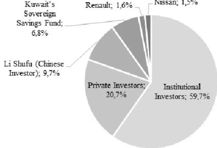
The chairman of the board of management is Dr. Dieter Zetsche, who has been a member of the board since December of 1998 and leading the company since 2006, after the demerger with Chrysler AG. The remuneration structure of the board is divided into three components, base salary (30%), short-medium term performance goals (30%) and long-term performance goals (40%), where board members are obliged to hold part of their remuneration in company shares, thus creating incentives to secure Daimler long-term success.
The ownership structure is rather diluted, with no shareholder holding a significant position, as seen in figure 1 above. As of December 2018, Daimler has 1.070 billion free floating shares, each giving 1 voting right. The firm shares are listed at the Frankfurt and Stuttgart stock exchanges and are part of the DAX 30 and the European Stoxx 50 indexes.
Figure 1 - Overview by ownership
19
3.1. Business Model
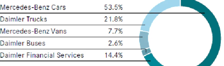
The group is divided in five business segments: Mercedes-Benz Cars, Daimler Trucks, Mercedes-Benz Vans, Daimler Buses and Daimler Financial Services. In 2018 had a total revenue of €167.4 billion, a 2% increase regarding the previous year.
Figure 2 - Daimler's 2018 revenue by division (total of €167 billion)
Source: Daimler Annual Report 2018 Mercedes-Benz Cars
The division with the foremost relevance in the group revenues is the Mercedes-Benz Cars, that comprises the supply of premium automobiles under the brands Benz, Mercedes-AMG and Mercedes-Maybach. It also includes the new electric mobility brand EQ, to be launched in the next couple of years, as well as the urban brand Smart. The company is best known for this division, which is the leader in its segment for the third consecutive year (2016-2018), with unit sales of more than 2.3 million vehicles in 2018, being China (28% of the unit sales), United States (14%), Germany (14%) and other European markets (28%) their core markets.
Daimler Trucks
Daimler is also the world’s largest producer of trucks above 6 metrics tons, that are comprised by the brands Freightliner, Western Star, FUSO and BharatBenz. Due to the similarities in production technology with trucks, the FUSO brand is also in charge of part of the production of buses. Regarding the main sales markets for this segment in 2018, those are the NAFTA region (37% of the unit sales, where most of the production facilities are located,
20
with 14 of the 26 in total), Asia (32% of unit sales) and EU 30 region (European Union, Switzerland and Norway, with 17% of sales).
Mercedes-Benz Vans
In this segment Daimler besides offering commercial solutions with the Sprinter large van, the Vito mid-sized van and the City urban delivery van, also targets the private costumer segment, with the Marco Polo camper van and more recently, in November 2017, launched the X-Class, which is the first premium pickup in its segment. This division has manufacturing facilities distributed worldwide, and its main region of sales is the EU 30, accounting for 66% of the division sales in 2018.
Daimler Buses
Daimler is the market leader when it regards to buses, more specifically above 8 metric tons, under the Mercedes-Benz and Setra brands. The core markets are the South-American and European ones, generating both almost 70% of the division revenue and in those regions are also located the 14 production facilities.
Daimler Financial Services
This division of Daimler provides financing and leasing solutions to end costumers, as well as insurance brokering, fleet management services and investment products. Furthermore, it is also responsible for several mobility services as the Moovel mobility platform, the Mytaxi app and the Car2go, the world’s leading car-sharing business. This division supported roughly 50% of the vehicles sold by Daimler in 2018 with their leasing and financing plans.
3.2. Sector Outlook
The automotive industry is being transformed by disruptive trends, that are going to shape our mobility in the near future. Digitalization is shifting original equipment manufacturers (OEMs) business model to providers of mobility services, and other non-traditional players are extending their business into the “connected car”, as it is represented in figure 3.
21
These technology-driven changes are being propelled by fast growing emerging markets such as China (which is the single biggest market for Daimler’s cars), the accelerated use of digital solutions and changing consumer preferences towards urban mobility. Hence, the trends one can expect in the automotive sector are autonomous driving, connectivity, diverse mobility and electrification, with total industry revenues amounting up to €6.7 trillion by 2030 (McKinsey, 2016). The combination of these four factors is expected to cause a revolution in the industry, and thus request a lot from an investment perspective.
Following this line of thought, Daimler has demarcated four strategic pillars in their growth strategy, they named as “CASE”: Connected, Autonomous, Shared and Electric, referring to the future fields of driving experience. These fields go hand in hand as they are interdependent. For instance, for autonomous driving to be possible, or ride-sharing to be efficient, it is necessary to have a vast software infrastructure that connects people and vehicles on the road.
For a better understanding of each one of these four pillars, please refer to Appendix 9.1. Figure 3 - Repositioning of several companies due to digitalization, with interest in the “connected car” product
22
3.3. Risks and Opportunities
Similar to every other business, risks and opportunities for Daimler will change according to supply and demand shifts. On the demand side, that is the consumer side, the main influences are the macroeconomic environment, political impacts, such as regulation and fiscal measures, and the industry specific demand already analysed above. As for the supply side one as to count with the production inputs, where the price of commodities like steel play a major role, among others.
This sector is cyclical and capital-intensive, and notwithstanding of having a solid reputation worldwide, Daimler faces rigid competition in all its segments, so it is of the outmost importance to keep investing in innovation. To assure their competitiveness, research and development expenses have been increasing for Daimler and accounts roughly of 5% of its revenues. By being one of the early adopters of new technology into the automotive space, Daimler is assuring to create a stronger customer base, strong technical and commercial legacies that will translate into higher revenues in the future, maintaining its pole position as the premium cars market leader.
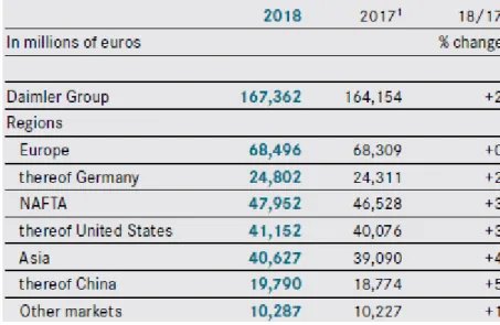
A great part of Daimler’s revenue is generated in the US (as seen in figure 4), and the current expansive fiscal policy could translate into a stronger growth in that area, boosting demand mainly of Mercedes-Benz cars and Financial Services segments. On the other hand, this could worsen the US debt situation, making the Federal Reserve to increase interest rates to offset inflation, thus increasing lending rates and decrease investment.
One other crucial area of business for Daimler is China, an emergent market, where it is reported that a new billionaire is arising every 5 days, thus, even though the automaker industry is a mature one, Daimler still has a great area of growth to cover in emergent markets, mainly in China, and the introduction of new electric vehicles will open the doors for more business opportunities. Nevertheless, as it operates almost worldwide, Daimler geographic risks are diversified and hence not exposed to any region conditions in particular.
23
Competition is also expected to increase, as connectivity becomes part of a vehicle, it is expected that tech companies start to deviate part of their business to the automotive industry, being one more competitor and taking a slice of the market share and revenue stream. However, the higher complexity regarding the technological future of the industry will mandate that incumbent players to be both competitors and to cooperate, sharing multiple infrastructures to reducing production costs. Regarding the competition coming from new mobility services, as ride sharing, this may result in a decline of private vehicle sales. Daimler decided to capture this new market, creating new brands, thus transforming this risk into more opportunities to create value.
There are some risks regarding production. On the one hand, additional costs can arise from unionized labour demands. On the other hand, raw material prices have featured some volatility in the past and price fluctuations will have an impact on overall economic profitability. The main ones used in the automotive sector are metals such as steel and aluminium, plastic and glass. Aluminium is lighter than steel (which still is the more used commodity in the production) and is being used as its substitute since it helps improve the fuel consumption, due to the emissions standards increasing regulation, but it is more expensive. Consequently, the price of metals will largely influence production costs, where raw materials are reported to be roughly 50% of manufacturing cost of vehicles (source: Statista).
Figure 4 – Daimler’s revenue by region
24
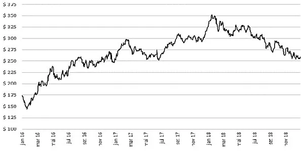
As a proxy for the price evolution of metals, please note the figure 5 below where the quotes of the Thomson Reuters Global Metal & Mining Index are presented. For the year of 2018 one can notice that there is a continuing decreasing trend, thus decreasing (or at least keeping constant) manufacturing costs. Also, Daimler is hedged against such commodities market risks (source: Daimler Website), being expected the overall cost to be constant over the next years.
Finally, costs relating to complying with new regulation, mostly regarding emissions, as discussed above, will represent a significant increase in risks, as noncompliance will reveal to be very costly.
3.4. Macroeconomic Outlook
From being a premium brand in its main segment, Daimler is less exposed to recessions as wealthier costumers spending is less sensitive to markets downturns. Also, it can pass more easily the burden of inflation (or new tax increases) to the consumer side due to this rigid demand. Nevertheless, in a cyclical sector, and since it is a long lasting good, demand should be higher in periods of expansion and the opposite in periods of recession.
In 2018 there was a decrease in automotive stocks performance, comparing to the previous analogous period, and Daimler was no exception. This fall has several causes, as there is an increasing geopolitical tension in several regions of the globe, beginning in an ongoing trade Figure 5 – Price quote of Thomson Reuters Global Metal & Mining Index (Jan16-Dec18)
Source: Thomson Reuters
25
dispute and subsequent punitive tariffs, mainly driven by the US government protectionist measures and countermeasures from China. This affects not only global demand, but also puts additional pressure on commodity prices, where exporters are starting to face a lower demand in China. Furthermore, the Brexit negotiations and Italy’s high national debt also had a negative impact on global stock markets and contributing to a rise in downside risks in global growth for the last semester of 2018.
In the USA, one will see a continuation of the tariff action on steel and aluminium, creating barriers for Daimler production, as well as the expansionary fiscal stimulus, which could give rise to unexpectedly high inflation, thus generating a stronger-than-anticipated monetary policy response, making the Federal Reserve to increase interest rates to offset inflation, where one would see increasing lending rates and decrease investment. One can expect a slowdown in USA growth from 2020, as the fiscal stimulus begins to unwind, being the expansion at its peak for the country. Advanced economies had a 2.4% growth in 2018 and are expecting to have a 2.1% in 2019 and 1.7% in 2020 (source: IMF).
In emerging markets, namely in Asia, medium-term prospects continue to be positive, with margins for steady growth, with expected increased capital flows from economies that are starting to stagnate or where expansion may have peaked. However, growth is expected to be lower in 2019, result of the trade measures. China GDP growth is of 6.6% and 6.2% (projected), for 2018 and 2019 respectively.
Following the rational above, the International Monetary Fund (IMF) stated that the prospects for the future remain optimistic, with the continuation of the steady expansion since mid-2016, and while financial market conditions remain accommodative in advanced economies, they could tighten rapidly if trade tensions and policy uncertainty intensify. The growth rates for global GDP have been revised, projected at 3.7% for 2019.
It is clear, as one can observe in figure 6, that in the past year and a half Daimler stock is underperforming comparing to the overall auto industry, which in turn is also one of the worst performing industries for 2018, contrasting to the upward momentum (also confirmed by increasing sales and revenue growth) for the last 10 years, since the subprime crisis in 2008. The performance was capture by using as a proxy the returns of the Thomson Reuters indexes for each industry.
26
3.5. Business Development
Daimler’s revenues and unit sales have been in an upward momentum for the last 10 years, since the Financial Crisis. However, for 2018, there was a small drop both in sales and revenue in the segment of Mercedes-Benz Cars following the slowdown of world economy, whereas the other segments continue to grow, but in a subdued way, comparing to the previous years (please see figure 7 and 8 below).
While in 2017 one could see a clear continuation of growth in sales, closely accompanied by a growth in revenue for all segments, the poorer demand in 2018 resulted in a decrease in performance for Mercedes-Benz Cars. This had several causes, beginning with an increased concern by consumers towards the auto industry with the introduction of the WLTP certification procedure. Then, in China, the largest market of this segment, sales were weaker due to the discontinuation of tax incentives for buyers of new small cars.
Source: Thomson Reuters
27
All the other segments, as shown in figure 8, had positive but smaller, growth in sales. This is in line with the stated above regarding world demand, where the economy reached its peak and stagnated in the second half of 2018.
Source: Daimler Annual Report 2018
Source: Daimler Annual Report 2018
Figure 8 – Daimler’s unit sales growth by segment (absolute value is shown; historical period)
28
4. Discounted Cash Flow Valuation
To compute the forecasts, historical figures were used for the last 3 years (2016, 2017 and 2018) as basis for the estimation. Daimler adopted new accounting standards (IFRS 9 and IFRS 15) in the beginning of 2018, and full adjusted financial figures were provided since 2016, enabling the comparison only from this date onwards. The introduction of IFRS 15 results in changes to revenue recognition, whereas IFRS 9 affects the recognition and measurement of financial instruments. Furthermore, as the auto industry has been renovating its characteristics, with the introduction of new regulations and innovative products, 3 years seems a reasonable time span, expected to have incorporated in its figures this recent industry changes.
The explicit period chosen was six years, as amongst the industry literature reviewed – for instance (McKinsey, 2016) – it is identified a revolutionary period towards 2030 in the automotive industry, and consequently a big need for investment up to 2025. This is also a consequence of 2025 being the year where the diesel vehicles are going to start to be banned from circulation.
4.1. Revenue Growth
Regarding the computation of the revenues for Daimler, it was done a sum of the parts (appendix 9.2.). This was done individually for each one of the segments, since different segments show different growth rates.
For the forecasted years, the assumptions were made individually for each segment, following the rational that different segments will have different growths. The revenues forecast was done by using estimates of future unit sales for the operational segments, given Daimler is going to keep its market share on the segments as the markets grow. Consequently, other assumption needed is that the relation between unit sales and revenue is also going to be perpetually constant for each segment. Both relations are stable as seen in the table of the appendix 9.2.
In regards of the outlook for trucks, as different information was available (market growth instead of market sales), it was used the market growth as the starting point, where it is expected a market CAGR of 3,1% in unit sales until 2024, with Daimler maintaining the lead position
29
(source: IHS Market). This value was used as growth base for the unit sales, despite of Daimler having a far greater growth in the last 3 years. This market is very volatile and thus a reasonable approach should be taken.
Financial Services are expected to grow at a CAGR of 2,7% 2018-2024, following the overall average relative sales of group units. The source for the forecast of car sales was Statista. For the vans, represented as commercial vehicles, was OICA (International Organization of Motor Vehicle Manufacturers).
Analysing each segment individually, Mercedes-Benz cars and vans are expected to generate a revenue CAGR of 2.8% and 3.7% respectively until 2024. This dissertation is of the opinion that the ban in diesel vehicles will not have an impact in the overall market sales, since electric and hybrid vehicles will be a key driver of industry growth.
Source: Own estimates
Figure 10 – Global monthly sales evolution of plug-in cars
Source – EV Volumes Website (Electric Vehicle World Sales Database)
30
Furthermore, this increase in sales is in line with the thought that Daimler is going to have a major role in the market revolution to come, where it is going to present several new hybrid and electric models, and even creating a whole new brand to face this new demand (please note the sales evolution in figure 10, where it is possible to see a substantial rise in hybrid vehicles sales).
China is probable to maintain the role of biggest market for Mercedes-Benz’ cars, as they are also one of the biggest investors in new technology, proven by the recent investments of Daimler in R&D and new factories in this location and more yet to come in the next years (already have settled the construction of a new electric batteries factory for €145 million, adding to the more than one billion spent in R&D only in China in the last few years).
This location will also be a key one in Daimler growth, since in 2018 Daimler has lost some momentum due to the increase in import taxes and the discontinuation of the tax incentives to buy new small cars, thus will be important to establish and increase the number of car dealerships there.
Although Daimler buses are estimated to grow at a CAGR of 9.6%, its revenue does not have a meaningful impact in the overall growth, being less than 4% of total revenues.
One important note in the revenue forecasted taken into account in the end was the group revenue reconciliation, comprising elimination of intra-group transactions, that should not be taken into account. This is also shown in appendix 9.2.
4.2. Cost of Revenue
Daimler’s cost of revenue has been constant throughout the years, as one can verify in figure 11, with a weight of circa 80% of revenues. Following the idea that Daimler can obtain raw materials at a fairly constant price, hedging against fluctuations, this weight was kept constant for the estimation period, using an average of the historical period.
31
Although one can argue that with the arrival of electric technologies the cost of production is expected to increase – McKinsey has estimated that the cost of producing an electric vehicle is, on average, higher in €12.000 than one of internal combustion engine - one should also note that this is going to be offset by higher revenues, having a nil impact when combining both factors, keeping gross profit fairly stable in percentage.
4.3. Other income statement assumptions
Other important assumptions regarding the income statement refers to forecasting general and administrative expenses, research and development costs (R&D) and the tax rate to be used. Since historically the weight of general and administrative expenses has had a clear linear relationship with revenue, that percentage was kept constant for the years to come. Regarding R&D, Daimler has stated that intends to spend close to €10b in the forthcoming years, thus the average growth rate for the historical period was kept until that level reached circa 5%, then kept constant for the remaining years, totalizing €10b in 2024. Finally, an average of the historical periods tax rates was used in the computations. Full income statement estimation is in appendix 9.3., where the remaining captions were computed as an average of the historical period, since their significance is also very low (for instance, other income and interests). Figure 11 – Daimler’s historical and estimated cost of revenue
Source: Daimler Annual Report 2018; Statistical analysis
Historical | Forecast 2016 2017 2018 f2019 f2020 f2021 f2022 f2023 f2024
Weight of expenses 10,2% 10,2% 10,2% 10,2% 10,2% 10,2% 10,2% 10,2% 10,2%
Weight of R&D 3,4% 3,6% 3,9% 4,2% 4,5% 4,9% 4,9% 4,9% 4,9%
Tax rate 30,1% 24,0% 28,4% 27,5% 27,5% 27,5% 27,5% 27,5% 27,5%
Source: Daimler Annual Report 2018; Statistical analysis
32
The trends above mentioned and expected to reshape the market will demand greater R&D expenses and Daimler has stated it expects to be a market leader, thus the need for innovation and producing better and more efficient vehicles, even on the level of in-car content.
In this way, Net income is expected to reach €8/9 billion, with the R&D expenses having a substantial weight until 2024. After this period, one might argue that the need for R&D should be lower, retrieving a higher EBIT in the years to come.
4.4. Free Cash Flow to the Firm
To arrive to the FCFF one must account with all the reinvestment needs, thus being necessary to estimate future capital expenditure and net working capital needs, as well as depreciation and amortization expenses.
4.4.1. Depreciation and Amortization
The caption of Depreciation and Amortization can be estimated using several methods according to (Koller, et al., 2010). Firstly, one can estimate depreciation as a percentage of revenues, a percentage of the net property, plant and equipment (PP&E) or based on equipment purchases and respective depreciation schedules if one knew beforehand the assets to be purchased. In this dissertation the method used was to estimate future periods PP&E along with the revenue growth rate and then to compute depreciation as a percentage of it (used the rate of the last year of the historical period to achieve a more accurate result). Same method was used to estimate amortization (of intangible assets).
Figure 13 – Estimation of Daimler’s FCFF
Source: Daimler Annual Report 2018; Statistical analysis
(in millions of euros) 2 016 2 017 2 018 f2019 f2020 f2021 f2022 f2023 f2024
EBIT 12 890 14 335 11 117 12 639 12 377 12 082 12 405 12 740 13 088
Tax rate 30,1% 24,0% 28,4% 27,5% 27,5% 27,5% 27,5% 27,5% 27,5%
(+) EBIT * (1 - tax rate) 9 005 10 897 7 956 9 161 8 971 8 757 8 991 9 234 9 486
(+) D&A - 3 092 6 846 5 414 5 815 6 245 6 707 7 203 7 737
(-) CAPEX 10 701 10 158 8 833 10 657 10 009 9 390 8 804 8 252 7 737
(-) Changes in NWC - - 3 306 1 608 975 1 033 1 069 1 107 1 146
33
4.4.2. Capital expenditure and changes in Net Working Capital
Future capital expenditures (capex) computation was based on the average percentage to revenues of the historical period, maintaining that ratio for the first forecasted year. Its evolution was divided between reposition capex and expansion capex, assuming Daimler will be in expansion until 2024. The decrease in expansion capex was done in a linear basis. The reason behind this rational is that Daimler has a big need for expansion investment, as explained in the beginning of this chapter, until it reaches steady state in 2025. Thus, the assumption that D&A will offset capex, related to a stable company is met only in the end of the explicit period. Investment in working capital were computed based on the assumption that the ratios Days Payables Outstanding (DPO), Days Sales of Inventory (DSI) and Days Sales Outstanding (DSO) would be kept constant as the last year of the historical period.
Other assets comprise deferred tax assets and tax refund claims, whereas other liabilities comprise deferred income, tax liabilities and deferred taxes. Thus, it is also necessary to Figure 14 – Estimation of future depreciation and amortization expenses
Source: Daimler Annual Report 2018; Statistical analysis
(in millions of euros) 2 016 2 017 2 018 f2019 f2020 f2021 f2022 f2023 f2024
TR days 25 27 27 27 27 27 27 27 27 Inventory days 76 72 80 80 80 80 80 80 80 TP days 35 35 39 39 39 39 39 39 39 Trade receivables 10 614 11 995 12 586 13 032 13 440 13 871 14 317 14 779 15 258 Inventory 25 384 25 686 29 489 30 234 31 178 32 178 33 214 34 286 35 396 Trade payables 11 567 12 451 14 185 14 543 14 998 15 479 15 977 16 492 17 026
Figure 15 – Estimation of the inputs for future net working capital
Source: Daimler Annual Report 2018; Statistical analysis
(in millions of euros) 2 016 2 017 2 018 f2019 f2020 f2021 f2022 f2023 f2024
Intangibles - net 10 910 12 620 13 719 14 914 16 212 17 624 19 159 20 828 22 641
Accumulated Intangible Amortization (7 437) (8 191) (9 616) (10 453) (11 364) (12 353) (13 429) (14 599) (15 870)
Amortization (754) (1 425) (837) (910) (990) (1 076) (1 169) (1 271)
Property/Plant/Equipment, Total -
Net 73 323 75 055 80 424 86 177 92 342 98 947 106 025 113 610 121 737
Accumulated Depreciation, Total (56 224) (58 562) (63 983) (68 560) (73 464) (78 720) (84 351) (90 385) (96 850)