UNIVERSIDADE DE TRÁS-OS-MONTES E ALTO DOURO
Curso de Mestrado em Instrumentos e Técnicas de Apoio ao Desenvolvimento RuralCONTRIBUTO PARA O PLANEAMENTO DO USO DO
FOGO CONTROLADO NA GESTÃO DE COMBUSTÍVEIS À
ESCALA DA PAISAGEM
Carlos Alberto Rodrigues Loureiro da Silva
Este trabalho foi apresentado na Universidade de Trás-os-Montes e Alto Douro como dissertação para obtenção do grau de Mestre no âmbito do Curso de Mestrado em Instrumentos e Técnicas de Apoio ao Desenvolvimento Rural na referida Universidade.
RESUMO
Um primeiro estudo foi realizado num povoamento de pinheiro bravo (Pinus pinaster). Os objectivos foram avaliar em que medida a aplicação de fogo controlado consegue uma redução na continuidade dos combustíveis ao nível da paisagem, e optimizar a sua distribuição espacial e temporal. O software FRAGSTATS foi utilizado para quantificar as mudanças na estrutura e na continuidade da do combustível na paisagem, associado à informação sobre a acumulação de combustível. Cenários alternativos em termos da distribuição espacial das áreas tratadas foram simulados utilizando uma abordagem com base na teoria de percolação. A fim de optimizar o efeito na redução da continuidade do combustível e analisar as configurações espaciais que minimizam a propagação de incêndios catastróficos, foi simulado o comportamento do fogo ao nível da paisagem com o software FARSITE. São propostas algumas recomendações para optimizar o efeito dos tratamentos no espaço e no tempo.
Um projecto de gestão de combustíveis ao nível da paisagem foi executado pelos Serviços Florestais na Serra do Marão, N Portugal. Descreveu-se o plano de tratamentos e usou-se o simulador de comportamento do fogo FARSITE para avaliar os efeitos sobre a propagação e comportamento do fogo na paisagem, em comparação com a situação pré-tratamento. O projecto de gestão de combustíveis foi concebido para uma bacias hidrográfica com 1728 ha, predominantemente ocupada por matos de Erica sp. e por jovens plantações de Pinus nigra. O tratamento com fogo controlado abrangeu 11,5% da bacia, criando um padrão de faixas de gestão de combustíveis parcialmente sobrepostas, com larguras de 70 a 120 m. Nas simulações foram utilizados modelos de combustível personalizados e um cenário meteorológico extremo para a situação pré-e pós-tratamento. No pior cenário (ausência de supressão e propagação nas faixas) o tratamento é bem sucedido em retardar propagação do fogo, mas aumenta a extensão da frente de fogo. A velocidade de propagação média e a intensidade da frente de fogo são reduzidas em 36% e 33%. A fracção da bacia hidrográfica onde o ataque directo teria sido ineficaz e eficaz, sofreu, respectivamente, uma redução de 41% e um aumento de 88%. As deficiências do projecto são discutidas, especialmente em relação à largura das faixas de gestão e projecções de fogo. Análise do resultado das simulações suporta o efeito positivo do tratamento de combustível na diminuição do potencial de incêndios severos e de grande dimensão.
Palavras-chave: Fogo controlado, dinâmica de combustíveis, fragmentação da paisagem, eficácia da gestão de combustíveis, simulação de incêndios na paisagem, Pinus pinaster
ABSTRACT
A first study has been carried in a maritime pine stand (Pinus pinaster). The objectives were to assess to what extent the application of prescribed burning achieves a reduction in fuel continuity at the landscape level, and to optimize its spatial and temporal distribution. The FRAGSTATS software was used to quantify changes in the structure and continuity of the overall fuel patch, coupled to information concerning fuel accumulation patterns. Alternative scenarios in terms of the spatial distribution of the burned plots were simulated using a percolation theory approach. In order to optimize the fuel continuity reduction effect of prescribed burning and examine spatial configurations that minimize catastrophic fire spread, fire behavior was simulated at the landscape level with FARSITE software. Some recommendations to optimize the PB effect in space and time are proposed.
A landscape-level fuel management project was implemented by the Forest Service in the Marão mountain range, NW Portugal. We describe the treatment planning and use the FARSITE fire growth simulator to assess its effects on landscape fire propagation and behaviour in comparison with the pre-treatment situation. The fuel management project was conceived for a 1728 ha third order watershed predominantly occupied by Erica-dominated shrubland and young Pinus nigra plantations. 11.5% of the watershed was treated by prescribed fire creating partially overlapped fuel breaks with widths mostly in the range of 70 to 120 m. Custom fuel models and extreme fire weather were used in the simulations for the pre- and post-treatment situation. In a worst-case scenario (absence of suppression and burnable fuel breaks) the treatment is successful in slowing fire spread but increases the fire front length. Mean rate of spread and fireline intensity are reduced by 36% and 33%. The fraction of the watershed where direct attack would have been respectively ineffective and effective by ground attack suffered a 41% decrease and an 88% increase. The deficiencies of the project are discussed, especially concerning fire break width in relation to spotting. Analysis of the simulation is supportive of a fuel treatment positive effect in diminishing the potential for severe and large-scale fire.
Keywords: Prescribed burning, fuel dynamics, landscape fragmentation, fuel management effectiveness, landscape fire simulation, Pinus pinaster
Índice
Lista de simbolos ... iv Lista de figuras...v Lista de quadros ... vi A. INTRODUÇÃO 1. Enquadramento...2 B. PUBLICAÇÕES 2 Prescribed Burning Planning at Landscape Level...62.1. Introduction ...6
2.2. Planning prescribed burning on the landscape ...7
2.2.1 Planning objectives. Fuel management and fire behaviour...7
2.2.2. Treatments shape and size...8
2.2.3. Where to place treatments in the landscape... 11
2.2.4. How much of the landscape should be treated? Operational and financial resources and treatment return interval ... 12
2.2.5. Spatial arrangement of fuel treatments ... 13
2.3 FlamMap simulator ... 14
2.4 Final remarks... 15
3. Spatial simulation of fire spread: two different approaches applied to Tapada de Mafra, CW Portugal ... 16
3.1. Introduction ... 16
3.1.1. Study area... 16
3.1.2. Objectives... 16
3.2. Fire simulators ... 16
3.2.1. Landlord – Spatial modelling system (version 1.2)... 16
The ModMED landscape fire modelling (Heathfield and Rego 1997)... 17
Factors that affect contagion probability ... 18
3.2.2. FARSITE - Fire Area Simulator (Finney 1998) ... 18
3.3. Methodology ... 20
3.3.1. Applying the ModMed fire model to some historical fire data from Tapada de Mafra ... 20
The simulation data and their preparation ... 20
Preparing the elevation grid map ... 22
Preparing the land use grid map ... 22
Estimating the fuel horizontal continuity... 23
Estimating the fuel moisture using riparian zones ... 24
Estimating the fuel moisture using aspect... 24
Winds ... 25
The damage maps ... 25
3.3.2. Applying FARSITE using custom fuel models developed for Tapada de Mafra... 26
The simulation data and their preparation ... 27
Landscape file... 27
Weather, wind and fuel files ... 27
3.4. Results... 28
3.4.1. Landlord fire simulation ... 28
3.4.2. FARSITE fire simulation ... 29
Output maps... 30
3.5. Conclusions ... 31
4. Optimizing prescribed burning to reduce wildfire propagation at the landscape scale ... 32
4.1 Introduction ... 32
4.2 Methods ... 33
4.3. Results... 35
4.3.1. Analysis of the prescribed fire effect in the 1993-1999 period... 35
4.3.1.1. Conclusion ... 37
4.4. Fire behaviour simulation using FARSITE ... 39
4.5. Final Recommendations ... 40
5. A simulation-based test of landscape fuel management alternatives in the Marão range of northern Portugal... 41
5.1. Introduction ... 41
5.2. The fuel treatment project ... 42
5.3. Objectives ... 43
5.4. Methods ... 43
5. Results and Discussion... 46
5.1. FARSITE simulation... 46 5.2. FlamMap simulations... 50 5.6. Conclusion ... 53 5.7. Final considerations ... 54 C. CONCLUSÕES 6. Considerações finais ... 57 Bibliografia ... 62 Agradecimentos... 66
Lista de símbolos
ASCII - American Standard Code for Information Interchange DEM – Digital Elevation Model
EUA – Estados Unidos da América FLI – Fire Line Intensity
GIS – Geographic Information Systems HC – Horizontal Continuity
LPI – Largest Patch Index
MIP – Mixed Integer Programming MPS – Mean Patch Size
MTT – Minimum Travel Time
NFFL – Northern Forest Fire Laboratory PB – Prescribed Burning
ROS – Rate of Spread
SIG – Sistemas de Informação Geográfica TOA – Time of Arrival
TOM - Treatment Optimization Model USA – United States of America
Lista de figuras
Figure 3-1. Raster landscape input layers required from the GIS for FARSITE simulation (Finney
1998). ... 19
Figure 3-2. Plan of steps used to run a FARSITE simulation ... 20
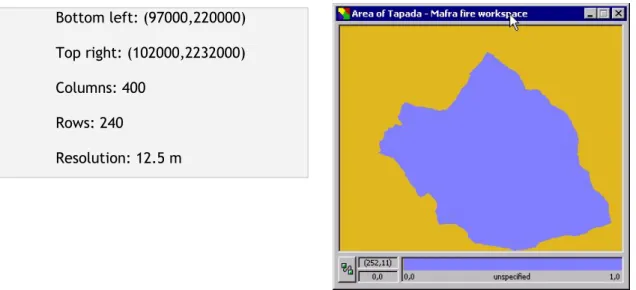
Figure 3-3. Grid specification and grid map of Tapada de Mafra area... 21
Figure 3-4. Digital elevation model (DEM) map of Tapada de Mafra area... 22
Figure 3-5. Land use map of Tapada de Mafra area. ... 23
Figure 3-6. Fuel horizontal continuity map of Tapada de Mafra area... 23
Figure 3-7. Water lines map and fuel moisture estimation. ... 24
Figure 3-8. Fuel moisture adjustment map using aspect... 24
Figure 3-9. Burnt area of the 1975 wildfire. ... 25
Figure 3-10. . Fuel models map of Tapada de Mafra. ... 27
Figure 3-11. Example of an output map of the simulation... 28
Figure 3-12. Fuel horizontal continuity (HC) model graphic and fuel HC map for Tapada de Mafra... 29
Figure 3-13. .Screen shot of FARSITE simulation result. ... 29
Figure 3-14. Graphic evolution of Burned area versus Time, during the simulation... 30
Figure 3-15 . Fireline intensity map, resulting from FARSITE simulation... 30
Figure 3-16. Rate of spread map, resulting from FARSITE simulation... 31
Figure 4-1. Distribution of PB areas by season in Perímetro Florestal do Entre-Vez-e-Coura.... 32
Figure 4-2. Prescribed burning active area and LPI (1993-1999)... 36
Figure 4-3. Prescribed burning active area and MPS (1993-1999). ... 37
Figure 4-4. Hypothetical modification of the spatial location of two plots in 1999. ... 37
Figure 4-5. Prescribed burning active area and LPI for the two scenarios. ... 38
Figure 4-6. Prescribed burning active area and MPS for the two scenarios. ... 38
Figure 4-7. Percentage of burnt area by fireline intensity, in the two FARSITE simulations... 40
Figure 5-1. Location of the prescribed fire units (left) and fuel model map (right). For the meaning of fuel model numbers see tables 1 and 2. Model 15 is NFFL 5 modified to represent Cytisus shrubland... 42
Figure 5-2. Proposal for fuel treatment location from the Treatment Optimization Model (TOM), respectively for SE wind (left) and upslope wind (right). ... 45
Figure 5-3. Fireline length and cumulative burned area in the watershed, before and after the fuel treatment, and as a function of time elapsed since the wildfire enters the watershed. ... 47
Figure 5-4. Fire front time of arrival before (left) and after (right) the fuel treatment. ... 47
Figure 5-5. Classification of fire behaviour before (left) and after (right) the fuel treatment: rate of spread (top, m min-1) and fireline intensity (bottom, kW m-1). ... 48
Figure 5-6. Watershed distribution (%) by classes of fire spread rate (right, m min-1) and fireline intensity (left, kW m-1), before and after the fuel treatment. ... 49
Figure 5-7. Cumulative burned area in the watershed, before and after the fuel treatment, and as a function of time elapsed since the wildfire enters the watershed. Left – SE wind; Right – upslope wind... 50
Figure 5-8. Watershed distribution (%) by classes of fire spread rate (m min-1), without treatment and after the two proposed fuel treatments for the SE wind (left) and upslope wind (right) scenarios. ... 51
Figure 5-9. Watershed distribution (%) by classes of fireline intensity (kW m-1), without treatment and after the two proposed fuel treatments for the SE wind (left) and upslope wind (right) scenarios. ... 51
Figure 5-10. Classification of rate of spread (m min-1) before and after the fuel treatments for the SE wind (top) and upslope wind (bottom) scenarios. ... 52
Figure 5-11. Classification of fireline intensity (kW m-1) before and after the fuel treatments for the SE wind (top) and upslope wind (bottom) scenarios. ... 53
Figura 6-1. Exemplificação do efeito do tratamento em parcelas adjacentes em anos consecutivos. ... 59
Lista de quadros
Table 3-1. Custom fuel models parameters (metric units) used in the FARSITE simulations... 26 Table 4-1. Variation in the active prescribed fire area and in the LPI and MPS indexes, for the
perimeter and global areas... 36 Table 4-2. Custom fuel models parameters (metric units) used in the FARSITE simulations... 39 Table 5-1. Custom fuel models for shrubland in the study area. ... 44 Table 5-2. Fuel models distribution and patch characteristics in the simulation area for the
pre-treatment. ... 44 Table 5-3. Landscape scenarios tested in the simulations... 45 Tabela 6-1. Esquema de delineamento para planeamento estratégico de gestão de combustíveis com recurso a simuladores de comportamento do fogo ... 61
1. Enquadramento
Esta tese de mestrado tem por base vários trabalhos sobre a temática do fogo controlado e do seu planeamento à escala da paisagem desenvolvidos no Grupo de Fogos da UTAD entre anos de 2000 e 2010, no âmbito de diversos projectos de investigação. Os capítulos seguem a sequência cronológica das publicações, relativas à aplicação do uso dos simuladores de comportamento do fogo para análise do efeito de tratamentos com fogo controlado em espaços florestais, para determinação das alterações no potencial de propagação de incêndios e comportamento do fogo associado.
No capítulo 2 faz-se uma revisão bibliográfica sobre o planeamento espacial (ou seja, ao nível da paisagem) de tratamentos de combustíveis, com especial ênfase no recurso ao fogo controlado. Este capítulo foi originalmente redigido como parte integrante do Deliverable 5.4.11 do Projecto Fire Paradox. Os objectivos do planeamento são quase exclusivamente orientados para a redução do perigo de incêndio. Modelos de comportamento do fogo e simuladores de propagação espacial do fogo são uma componente essencial no processo de decisão. Permitem uma análise à escala da paisagem, para determinar os locais mais eficazes e arranjo espacial dos tratamentos, com base na topografia, e cartografia e características dos combustíveis.
Diferenças estruturais da propriedade florestal e dos objectivos da gestão florestal são evidentes entre as regiões mediterrâneas do continente europeu e os constrangimentos que se impõem à gestão de combustíveis em países como EUA e Austrália, onde esta temática tem sido mais investigada. Considerações de ordem prática (recursos disponíveis, acessibilidade, e as restrições ambientais e sociais) são componentes necessárias no processo de tomada de decisão. Estas restrições podem interferir com os resultados dos modelos e simulações, ao ponto de serem mais relevantes na decisão final.
A expansão do uso dos Sistemas de Informação Geográfica (SIG) e sua aplicação à análise de risco de incêndio florestal levaram à necessidade do uso de simuladores para o comportamento do fogo que produzem resultados gráficos (mapas), para posterior análise e incorporação na cartografia de perigo de incêndio, e como ferramentas para apoiar os planos gestão florestal, na prevenção e defesa da floresta contra incêndios.
O capítulo 32 tem por base uma primeira aproximação à utilização de programas de simulação de propagação do fogo, que visa comparar duas abordagens diferentes para a simulação de incêndio. Uma abordagem muito simples, desenvolvida no âmbito do projecto europeu ModMed3, e funcionando como um módulo do software Landlord – spatial modeling system v1.2. O outro, FARSITE – Fire Area Simulator, com mérito confirmada pelo amplo uso
em diferentes países. Estas duas abordagens foram aplicadas à área de estudo da Tapada de Mafra, beneficiando da existência da necessária informação de base, recolhida no âmbito do projecto ModMed.
O capítulo 44 aborda a utilização do fogo controlado em povoamentos de pinheiro bravo (Pinus pinaster). A área de estudo escolhida foi parte do Perímetro Florestal de Entre-Vez–e-Coura. A escolha desta área foi determinada pela existência de parcelas de tratamento com fogo controlado, documentadas para o período de 1993 a 1999. Esta é uma das áreas pioneiras no uso do fogo controlado em Portugal, tendo sido utilizada como banco de ensaio para uma série de estudo sobre os efeitos do fogo controlado.
Os objectivos foram avaliar em que medida a aplicação de fogo controlado em parcelas dispersas se traduz numa redução na continuidade dos combustíveis ao nível da paisagem, e optimizar a sua distribuição espacial e temporal. O software FRAGSTATS foi utilizado para quantificar as mudanças na estrutura e na continuidade do combustível, em associação com informação sobre os padrões de acumulação de combustível com o tempo.
Cenários alternativos, em termos da distribuição espacial das áreas tratadas, foram simulados, utilizando uma abordagem baseada na percolação. Procurou-se optimizar o efeito do fogo controlado na redução na continuidade da carga de combustível, e analisar as configurações espaciais que minimizam a propagação de incêndios catastróficos. Para este efeito foi simulado o comportamento do fogo ao nível da paisagem com o software FARSITE. Algumas recomendações para optimizar o efeito do fogo controlado no espaço e no tempo são propostos.
No capítulo 55 examina-se um plano de tratamento de combustíveis ao nível da paisagem, implementado na área da Serra do Marão, norte de Portugal. Este plano representou em 2005 uma alteração na aplicação do fogo controlado para gestão de combustíveis. Foi o
2 Loureiro, C., P. Fernandes, A. Lopes, D. Heathfield, F. Rego, 2001. Spatial Simulation of Fire Spread:
Two Different Approaches Applied to Tapada de Mafra, CW Portugal. In "Proceedings: Workshop - Tools and Methodologies for Fire Danger Mapping", p.41-53. 9 - 14 Março, 2001. UTAD, Vila Real.; Loureiro, Carlos and Duncan Heathfield. 2000. Using the fire model for Mafra. Online in
http://www.worldinabox.co.uk/ModMed/FireModel/index.htm (accessed March 2001)
3ModMED – Modelling Vegetation Dynamics and Degradation in Mediterranean Ecosystems. European
Commission DG-XII
4 Loureiro, C., P. Fernandes, e H. Botelho. 2002. Optimizing prescribed burning to reduce wildfire
propagation at the landscape scale. In Proc. IV Int. Conf. on Forest Fire Research & 2002 Wildland Fire Safety Summit, Viegas, D.X. (Ed.), Luso, 18-23 Nov. Millpress Science Publishers, Rotherdam.
5Loureiro. C., P. Fernandes, P. Mateus e H. Botelho. 2006. A simulation-based test of a landscape fuel
management project in the Marão range of northern Portugal. In Proc. 5th Int. Conf. Forest Fire Research,
primeiro executado numa perspectiva de planeamento à escala da paisagem. O efeito do tratamento sobre o potencial de incêndios é avaliado com o software FARSITE, em comparação com o cenário de pré-tratamento de combustível.
Uma alternativa ao plano de gestão implementado foi obtida utilizando o software FlamMap, através da ferramenta Treatment Optimization Model (TOM). Em seguida, usou-se novamente o FlamMap para comparar a eficácia do tratamento efectuado no terreno com a proposta de optimização para dois cenários distintos de simulação fogo. Um cenário de propagação dominada pelo vento, usando mapas de vento produzidos no software WindNinja, e um segundo cenário com a propagação dominada pela topografia. O efeito dos tratamentos nas características do comportamento do fogo foi obtido a partir dos resultados das simulações, e comparado para os dois cenários.
2 Prescribed Burning Planning at Landscape Level
2.1. Introduction
Fire is an important part of Mediterranean ecosystems and forest fires have always been present in southern Europe rural areas. However, in the past, fire expression in the landscape was related with land use and space occupation, in a time when humans were substantially more present in rural areas. Such influence constrained fire size, since the intense use of forests and their resources was effective at increasing spatial heterogeneity and decreasing flammability, hence decreasing landscape vulnerability to fire.
Demographical and land use changes over the past decades have led to dramatic changes in the fire regime, both nationally and throughout Europe, especially in the Mediterranean basin. New challenges arise in regards to forest and fuel management, which are constrained by scarce human resources and decreasing funding. It doesn’t help that the political response to the wildfire problem privileges investment in fire suppression, which paradoxically can contribute to larger and more severe fires in the future (Fernandes 2008).
The use of prescribed fire as a fuel management technique in Europe dates back from the 1970’s, and was inspired in the United States practice. The first extensive prescribed fire management program was launched in Portugal. However, the traditional use of fire in wildland management is old and deeply rooted in rural communities throughout the Mediterranean, especially to renew and maintain rangelands in mountain areas.
Diverse studies in the western Mediterranean have been carried out since the 1980’s to characterize the environmental effects of prescribed burning. The burning conditions commensurate with the achievement of management objectives have been defined, and the importance and appropriateness of prescribed burning to manage European Mediterranean ecosystems is now recognized.
Prescribed burning planning is carried out at two different scales. At the plot/stand level, is focused mainly on the prescription that leads to specific treatment effects. The other, at the landscape scale, where planning should address the strategical location of treatments to protect the greatest value areas from the effects of catastrophic wildfires (Hunter et al. 2007), limiting wildfire spread and providing more opportunities to effective fire suppression. Finney and Cohen (2003) suggest to differentiate wildland-urban-interface environments, where planning should take into account the combination of built structures and vegetation areas.
optimization, especially for fuel management and fire hazard mitigation. Prescribed burning planning at the landscape scale implies several questions related with burn objectives and fire use restrictions. Other constraints to consider are common with fuel management planning in general, regardless of the treatment used.
Several issues directly restrain the applicability of prescribed fire (Fernandes and Botelho 2003). There are restrictions on the use of fire on a large scale in relation to its effect on air quality and local residents health (Agee and Skinner 2005), or on the use of fire in wildland-urban interface areas, which offers additional difficulties due to increased complexity of social and technical issues, and where most of the effort focuses on the need for planning and coordination prior to the burn operation (Miller and Wade 2003). This same complexity is apparent in the Mediterranean basin, due to patterns in land use type and objective, land ownership, and human occupation. The demand for skilled personnel and the necessity to respect meteorological windows of opportunity and ecological restrictions, as well as a tighter legal framework, further increase the limitations in comparison with alternative fuel treatments.
2.2. Planning prescribed burning on the landscape
2.2.1 Planning objectives. Fuel management and fire behaviour
The continual accumulation of biomass, that fuels wildfires, points to the need of developing fuel management strategies at the landscape level which are effective at decreasing the size and severity of wildfires (Weatherspoon and Skinner 1996). In a country like USA the fuel build-up problem is mainly related with a fire suppression policy, where the role of fire as an ecosystem process and “manager” has been negated. Concurrent favourable weather conditions lead to an increase in the area burned by high-severity fires (Weatherspoon and Skinner 1996). Fire suppression policies are also in place in Europe. However, the major cause for the high levels of biomass accumulation is related with agricultural land abandonment and the absence or reduced intensity of forest management.
The purpose of fuel management is to modify the behaviour of a future wildfire, by decreasing fuel load and changing vegetation structure. The expected changes in fire behaviour are decreases in rate of spread, fire intensity and crown fire potential. A meaningful change in wildfire behaviour, i.e., a change that will benefit fire suppression, implies that the treatments are effective both locally and in the overall landscape. However, treatment of the entire area is not feasible and its extent is limited by economic, structural, physiographic and ecological constraints. Fuel management needs to be consistent with other management objectives, which can be complementary to wildfire prevention, such as rangeland management, control of pests and diseases and ecosystem sustainability (Hunter et al. 2007, Weatherspoon and Skinner 1996).
The best possible solution for protection against wildfires may not be feasible due to impacts on wildlife, watersheds, or scenic quality objectives (Gercke and Stewart 2006).
Planning should be carried out in the long term, in a sustainable way in order to maintain treatments efficacy over time (Hunter et al. 2007), and in this context it is important to know the period of treatment effectiveness in changing fire behaviour, i.e., which is the time required to recover to a hazardous condition. Treatments should start in the most logical, effective and economically efficient places (Weatherspoon and Skinner 1996). We should consider the implementation of the treatment areas in the landscape, its geometry and the relative position of treatment units. The strategic location of treatments has to maximize their effect in fire behaviour, allowing safe fire fighting and, in some favourable situations, self-containing wildfires.
2.2.2. Treatments shape and size
Two general strategies for landscape-scale fuel treatment can be considered: fire-breaks and fuel-fire-breaks with the main objective of stopping fire spread, or area-wide treatments that form a mosaic of scattered treatments where fire behaviour is modified (Finney 2001). Longitudinal, long and narrow plots that are placed perpendicularly to the main direction of fire spread are the most common spatial strategy of fuel treatment. Traditionally, the implementation of fuel management areas follows this linear pattern of fuel-break, designed to limit wildfire growth, but also as anchor points for indirect attack actions or prescribed burning in neighbouring areas (Agee et al. 2000). This is the tradition in European countries of the Mediterranean, such as Portugal, France and Spain (e.g. Rigolot 2002a), or in some USA regions (Agee et al. 2000), with variation between countries. In Australia, where the areas treated by prescribed fire are typically larger, area-wide treatments are prevalent and have been shown to be effective in decreasing the incidence of large wildfires (Boer et al. 2009).
The aim of each treatment unit is not to stop a fire spreading, but reinforce fire suppression actions (defensible locations) and thus reduce the size of the fire, helping the safe use of indirect attack techniques, including back-fire, but having little effect on fire behaviour and severity outside the treated area (Agee et al. 2000, Finney 2001).
An assessment of fuel-break effectiveness in southern France (Lambert et al. 1999) identified some factors favourable to fire fighting success, namely the quality of the access (location, width and conservation status), fire-fighting resources available on site and synergy between ground and air resources. The following negative factors are mentioned: detection delay (at initial attack level); limited access; herbaceous fuel load (implying faster fires); and the existence of fine fuel pockets, which favour spotting. Therefore, fuel-breaks should be
implemented with the support of roads or tracks, allowing access by fire suppression resources, and regular treatment of fuels.
Duguy et al. (2007) have analyzed the effect of different alternatives for implementing a fuel-break network, suggesting that these structures are effective in reducing wildfire size, but do not reduce the rate of spread or intensity of the fire front. Fuel-breaks by themselves are only successful in slowing the progression of the fire (Finney and Cohen 2003) and significant loss of value may occur within a block bounded by a treated strip only (Agee et al. 2000).
Fuel-breaks can be viewed as the starting point for landscape-level fuel management. Subsequent and more extensive treatments will gradually decrease the fire damage potential within the treated areas (Agee et al. 2000). According to the same authors, a network of connected fuel-breaks is complex. A wildfire will more likely find a fuel-break segment if it’s planning took into account factors such as the potential for ignition and the values at risk. Otherwise, if the pattern of firing events is random and values are regularly or uniformly distributed on the landscape, an approach based on a network of fuel-breaks is always preferable.
Fuel-break features (Finney 2001): 1) Established to help contain fires.
2) Reinforce defensible locations determined prior to fire occurrence. 3) Facilitate indirect suppression tactics, including backfiring.
4) Reduce fire size.
5) Have little effect on fire behaviour or severity outside the treatment area. 6) Burnout operations may lead to larger wildfires and larger areas burned severely.
On the other hand, fuels management planning can result in treatment units spread over the landscape in strategic locations to maximize the benefits gained from changes in fire behaviour (Finney 2001, Parisien 2007). Finney (2001) suggests a pattern for treatments distribution where the treated units overlap in the prevailing direction of fire spread. This pattern is expected to generate fragmentation of extreme fire effects, as the fire front is fragmented by the treatment units.
Partial overlap treatment features (Finney 2001)
1) Treatment unit size is unimportant. Only the relative dimensions of the pattern affect fire spread rate trough the pattern. The effect is related with distance between plots and the extent of overlap.
2) The distance between units in the heading direction must be smaller than the wildfire width.
3) Fire spread rate inside the treated area must be slower than in the untreated landscape.
4) A lower percentage of the total area requires treatment as treatments become more effective.
The location and purpose of prescribed burning treatments must decide the units optimal shape. Prescribed burning productivity depends of the area treated per unit of time, which is directly proportional to the ignition line length. The use of anchor points based on existing structures (such as tracks, roads...) can decide the shape of units, optimizing resources and avoiding construction of containment lines.
Spot fires are one of the main concerns in defining treatment size. However, site physiography and type of vegetation can constrain and even determine the optimal size of the treatment units. When the treatments seek to contain a wildfire (as in fire-breaks), their width is often determined by empirical rules or by local experience and dozer size (Davison 1988). There are no default values for fuel and fire break widths. Earlier references (1960 and 1970’s) in the U.S.A. indicate values ranging from 65 to 300 meters (references in Agee et al. 2000). However these widths can be smaller, like in fire-breaks in Australian grassland (2-5 t.ha-1 and 0.15 to 0.55 m height) which range from 5 to 15 m (Davison 1988), based on a model for the probability of fire break breach based on fire intensity, the presence of trees within 20 m fire break width (Wilson 1988). When implementing a fuel-break network, the size of the different sections may be variable, with subdivisions closer to the most remote, and would function primarily as anchor points for the use of prescribed fire (Agee et al. 2000). In France, expert opinion identified fuel-break width, shrub volume and tree cover as the most discriminating criteria to assess fuel-break effectiveness (Rigolot 2002a). Finney (2007) indicates a treatment units range from 800 to 2500 m, or 65 to 390 ha.
Flexibility in treatment size is important when planning for different landscapes, topography, ecology or constraints. When treatments follow a pattern of dispersed units that overlap partially, the size of the treatment is theoretically independent of scale, i.e., the effect of treatment size is only related with distance between plots and the extent of overlap, which must be less than the fire front width (Finney 2001).
2.2.3. Where to place treatments in the landscape
The distribution pattern (topological and spatial) of treatment plots in the landscape is a major factor to consider when optimizing treatment location, to maximize the effect on fire behaviour and fire hazard reduction (Finney 2001, Noonan 2003, Hunter et al. 2007). Treatment location is usually based on ecological objectives, convenience, cost, ownership or accessibility (Finney 2001). Fuel-breaks are usually located where indirect attack tactics are applied, such as along ridges and roads along valley or slopes (Agee et al. 2000).
The choice of treatment units based on topographic attributes and watershed area, and the use of terrain features such as water lines and ridges to delineate areas of treatment is consistent with the natural boundaries of wildfires (Mislivets 2003, Taylor and Skinner 2003). Duguy et al. (2007) suggest that wildfire spread is reduced by increasing the connectivity between dense forest patches with low fuel load, and promoting patches with more complex shape. Such complexity in burned plots shape is often find in Portugal where fire is traditionally used in range management, and where fire self-extinguishes due to changes in weather conditions or fuels.
Fragmentation of hazardous fuel areas within lower fuel load areas or less flammable vegetation types can be an effective method to reduce the size and intensity of fires, promote biodiversity and landscape resilience to fire (Burrows and van Didden 1991, Brockett et al. 2001, Duguy et al. 2007)
If operational and financial resources allow maintaining in a treated condition 30-40% of the landscape then the spatial pattern of treatment is unimportant, and the difference between randomly distributed treatments and an optimized spatial distribution of treatments is not significant (Finney 2007).
Some studies model fire growth under different treatment scenarios to determine the optimum location of treatments (Finney 2001, Agee et al. 2000). Finney (2007) proposes an algorithm to optimize the location of fuel treatment units to prevent the spread of large fires. The method requires two spatial data sets:
1) The current fuel situation;
2) The potential fuel situation, after treatment in an area previously identified as possible to treat.
The difference in fire spread across the landscape between these two scenarios, under identical weather conditions, indicates where the treatments are effective in slowing fire growth.
2.2.4. How much of the landscape should be treated? Operational and financial resources
and treatment return interval
To decide the burning rotation period, three factors must be weighed (Keeley 2002): 1) The competence of skilled personnel to safely maintain fire within the planned boundaries;
2) Vegetation likelihood to ignite and sustain fire spread.
3) And finally, for how long will the treatment persist, i.e., for how long it will be effective in reducing fire danger.
Fire behaviour in the landscape changes above a fuel type composition threshold (Bevers et al. 2004, Duguy et al. 2007). In randomly allocated treatments, effectiveness is related to the treated area fraction (Finney 2003, Bevers et al. 2004) and aggregation (clusters) of treated units. The more aggregated the treatments are, the largest proportion of the area must be treated (Bevers et al. 2004).
Fire severity in treated areas increases with time since treatment (e.g. Fernandes et al. 2004). However, other factors can affect fire severity, e.g. Finney et al. (2005) report decreases with treated plot size and number of previous prescribed fires. Prescribed burning is more effective in reducing surface fine fuel (Lambert et al. 1999), and a seasonal distribution allows a variety of burning conditions that reflects in the size and intensity of prescribed fires, and in the spatial and temporal distribution of this variation (Brockett et al. 2001). Consequently, the season of burn can have implications on the treatment return interval.
Maintenance treatments frequency varies with region and vegetation type and can be determined from historical fire regimes or from the rate of fuel accumulation (Hunter et al. 2007). In southern France, efficient fuel-breaks require treatment intervals of 3 to 4 years, as judged from shrub volume (Rigolot 2002a). Several examples of treatments longevity indicate that prescribed burning reduces the severity of wildfire for 2 to 25 years after treatment (Hunter et al. 2007).
The annual treatment rate, or maintenance, should be high enough to compensate or overcome the temporal decrease in effectiveness. Finney (2007) proposes that the annual treated area fraction should be 1/n, where n is fuel recovery time (years). E.g., if n=4 years, then the area treated every year should be 0.25 of the total percentage of treated landscape. If the total percentage of treated landscape is 20% (which roughly cuts the area burned to half if the treatments are strategically placed), then 5% should be treated annually. Note that if the treatment pattern is random then the treatment effort would have to double in order to achieve the same effect (Finney 2007).
2.2.5. Spatial arrangement of fuel treatments
Some authors have studied the topic of fuel treatment planning on the landscape, suggesting different methods to optimize the effect of treatments. Normally the process of identifying priority areas for treatment is based on a multiple criteria weighted analysis, and using GIS analysis for criteria selection planning.
Keifer et al (2000) propose a model based on GIS analysis, incorporating ecological role of fire in fire management planning, together with fire risk and hazard. The process includes information about vegetation, fire return interval and fire perimeters from historical records. The result is an index that ranks potential areas for treatment based on the need to restore fire disturbance to its historical range, and allows setting treatment priorities.
Hiers et al (2003) also propose a process for identifying priority areas for the use of prescribed burning, on the basis of key conservation criteria and landscape scale management objectives. The model incorporates the experience of managers and specialists that identify and rank criteria according to the burn priorities. The ranking is dynamic and adjustable to the treatment units limits. The criteria used include time since last fire, site quality, time since treatment for ecosystem restoration and land use classification. Through the use of a GIS, the criteria are weighted according to their relative contributions, leading to a global prioritization of landscape scale burning.
The methodology of MacGregor et al. (2003) to develop fuel management projects involves a set of design decisions, aimed to a broad range of objectives, outlined as evaluation criterion. These criteria may include environmental, economic (including cost), social and risk-related factors. The optimal design is the one that best reflects the alternative value (trade-off value) of that option, coupled with the relative weight or priority assigned to the criterion. This assessment can include a variety of purposes including: a) what is the potential advantage of one plan over another, b) the extent to which a set of plans covers all the objectives, c) where, within the objectives, there may be need to develop new plans. The fuel management program is considered as a portfolio of plans, each rated in terms of benefits and risks.
For Bevers et al (2004) the objective is to create fuel-breaks in the landscape, from a pattern of spatially correlated random treatments. From a map of the treatment area, divided into a grid of cells that represent potential treatment sites, the cells to be treated are randomly selected, using an algorithm that provides, optionally, a greater degree of aggregation of random treatments. However this means that a larger number of randomly treated grid cells are probably needed than if the locations of treatments were chosen strategically.
Wei et al (2008) proposes a mixed integer programming (MIP) for locating fuel treatments on the landscape, based on spatial information of ignition risk, conditional probability of fire spread (between raster cells), fire intensity and values at risk. The
particularity of the model is that fuel treatment locations are not selected based on location and behaviour of specific fires, but fire hazard is assumed to be cumulative over the landscape, along the direction of maximum spread (wind direction). From this assumption the model locates where the treatments are more effective in reducing the fire hazard accumulation. The available budget constrains the amount of treated area.
2.3 FlamMap simulator
Some of the planning strategies consider the identification of higher-risk areas or where the probability of fire is higher. The identification of these areas defines critical candidate areas for treatment and also treatment priorities. Expansion to wider areas in the landscape can subsequently take place from the priority areas.
FlamMap (Finney 2006) is a software that simulates fire behaviour in the landscape and a reference in fire hazard classification and mapping. It can be used to identify the areas where fire hazard is greatest, to support decision, and for validation and optimization. FlamMap includes a module that proposes the best locations for fuel treatments with the goal to stop the spread of large forest fires. It also provides information on: 1) minimum travel time; 2) major fire travel routes; 3) opportunity for treatments; 4) percentage of land area to be treated.
The Treatment Optimization Model used in FlamMap proposes area-wide treatments (or a pattern of dispersed treatments), supported on treatment units topology to reduce the spread and intensity of fire. Its main features are:
1) Fire behaviour and effects are modified, wherever fire reaches a treatment unit; 2) Fire suppression is facilitated;
3) Dispersed treatments slow fire growth, and facilitate the establishment of
containment lines in a wildfire event;
4) Fuel treatment units limit fire spread in the heading direction, which results in the
greatest reduction in fire size and severity;
5) The topology of the treatment units is part of a spatial pattern that reduces fire
spread rates and intensities.
The importance of rate of spread for each fuel type requires that treatment planning should target specific weather conditions. Weather conditions that should be considered by the planning scenario are those that historically have led to large and severe wildfires.
The spatial pattern and dimensions of treatments on the landscape should be guided by the history of wildfire events (e.g. size distribution, dominant direction of spread, weather conditions). The most efficient partially overlapping pattern is based on this information and
generates a spatial pattern of treatments that overlap perpendicularly to the main direction of fire spread under the targeted weather conditions. To maximize this effect, with restrictions for treatment location, size and percentage of treated area, the treatment pattern that originates the greatest reduction in overall fire spread rate with the minimum treated area is taken into account. Because treated areas are not connected, the procedure is more flexible in accommodating spatial variability and constraints.
FlamMap is used to produce maps of rate of spread, flame length and fireline intensity. GRID files for altimetry, slope and aspect are created from the digital terrain model. This information is joined with fuel model maps to form the LANDSCAPE file, the mapping base to FlamMap simulation, supplemented by information on weather, wind and fuel moisture. Fire behaviour metrics (rate of spread, flame length and fireline intensity) can be calculated for different scenarios. This information is calculated using the Minimum Travel Time (MTT) algorithm which calculates and chooses the fastest fire paths using a two-dimensional model of fire spread/growth. The model determines the growth and behaviour of fire for the set of fire paths with the shortest delay time from the ignition source set. During the simulation weather and fuel moisture variables are kept constant.
2.4 Final remarks
Fuel treatment planning is a theme that has been object of managers and researchers attention. This interest is recently growing, motivated by the increasing occurrence of extreme large wildfires. This scenario, associated with the scarcity of resources and changes in the social and economic framework, which has led to a growing attempt to optimize fuel management planning. Prescribed burning is one of the most appropriated treatment techniques, considering the actual framework.
The increasing availability of decision support tools and digital information has led to the development and application of simulators, complementary with traditional planning methods. The use of this simulatores should be validate by it’s applications to real cenarios.
3. Spatial simulation of fire spread: two different approaches applied to
Tapada de Mafra, CW Portugal
3.1. Introduction
Diferent tools to simulate the spread of forest fires have been developed in recent decades, driven by vulgarization of the information in digital format, and particularly with the incresing development of Geographic Information Systems (GIS).
In this initial approach, we tested the use of two fire spread simulatores applied to the landscape of Tapada de Mafra. In a simple way, we test FARSITE, fire area simulator (Finney 1997) and Landlord, spatial modelling system v1.2 (Heathfield 1999), using available information and developing the required inputs..
3.1.1. Study area
Tapada de Mafra is a public land estate with 834 ha, located in CW Portugal, north of Lisbon. The soil occupation is varied, being constituted by pure mixed stands of Pinus pinaster,
Pinus pinae, Quercus suber and Eucalyptus globules, and riparian vegetation areas along the
main water lines. A significant area is occupied by shrublands (Erica sp., Ulex sp.) and rangelands for wildlife feeding. The estate is surrounded by a high wall which serves as an effective fuel break for surface fires.
3.1.2. Objectives
The existence of a GIS for Tapada de Mafra area provide necessary data to use in simulations of fire behavior at landscape level.
The purpose of this study was to test the application of two distinct systems for simulation of fire propagation and production of maps of the affected area.
3.2. Fire simulators
3.2.1. Landlord – Spatial modelling system (version 1.2)
Landlord is a component-based, open-architecture spatial modelling system. It’s implemented as Windows software. It looks a bit like a GIS, but is quite different. In Landlord
maps are objects, not files. Landlord accepts .bmp or .img format images. Map objects reside in map collections. Map collections interact with spatial processes, which take one or more maps as inputs and make changes to one or more maps as output. All of these components are organised and configures within workspaces which can be saved and reopened (Heathfield 1999).
The ModMED landscape fire modelling (Heathfield and Rego 1997)
Landlord software uses a specific process to simulate the spread of fire, the ModMED landscape fire modeling, describing the value of variables with values
The landscape is represented using a raster mapping system, which is a grid of maps with variables values assigned to pixels. In modelling fire at the landscape level, we are simply trying to predict the extent of spread of a fire once it started. The role of the landscape fire model is to come up with a list of cells (pixels) which have been fire-affected by the time the fire goes out. The fact that it only interested in predicting the extent of spread makes the requirements, and therefore the approach, slightly different from most other fire models, which are usually concerned with predicting the rate of spread.
Model treats the fire event as instantaneous. Although it is obvious that an actual fire event takes at least some time to occur, the model treats fire as an instantaneous event. Wind speed and direction are constant for the duration of simulation. The sequence in which the pattern is developed is not intended to correspond to any likely sequence of fire pattern development in an actual fire. The sole objective of the simulation is to predict the damage pattern which results when the fire has gone out.
In order to predict the extent of a fire, the simulation is iterative, which means that a set of calculations are performed over and over again to produce a result. At the first iteration, when the fire begins, the fire starts in one or more cells. Each raster cell which is alight (a
source pixel) has one opportunity to ignite any adjacent cell, which are not alight (target pixel). Depending on the conditions, the model calculates a probability value (0-1) for the
spread of fire from source cell to each target cell - the contagion probability. A random number (0-1) is generated, and if this is less than the probability calculated, then the target raster catches fire. At the end of each iteration, the source pixels stop being on fire and the newly alight target pixel become the new source cell. As long as there are still cells alight, the simulation continues by beginning another iteration. When there are no pixels left alight, the simulation finishes, and a list of burned pixels has been collected. This approach handles fire as a contagious process
Factors that affect contagion probability
These are the factors which are used to calculate the probability of contagion: 1. Slope
2. Wind (speed and direction) 3. Fuel horizontal continuity 4. Fuel moisture content.
A factor value is calculated for each, and then each factor value is weighted according to the model configuration.
Topographic effect is expressed by the effect of slope. If the source cell value is lower than in neighboring target cell, it is likely that the fire spread successfully between the two. Slope influence is more effective for steeper scenarios. Contagion probability is reduced where the slope, in the direction of fire spread, is downhill, and increased when it is uphill. The model establishes a nonlinear relationship between the slope and the slope factor value.
The wind speed and direction are defined constants for the simulation. If the wind is blowing strong and with direction of fire propagation, increase the effect on ignition between ignited cell and target cell, the probability of progression is greater and the contagion probability increases.
The effect of the fuel is expressed through two factors: fuel humidity and horizontal continuity.
The horizontal continuity of fuel is a structural property of vegetation. The model expresses these values in a raster map. A low value indicates a patchy or discontinuous distribution, and thus the probability of infection is lower. The fuel moisture reflects the state of vegetation, determining the probability of extinction in a cell. The model combines the two factors providing a single fuel factor.
Each of these three factors can be weighted by the user in the configuration options. Model use these three factors multiplied and raised to the power 1/3 (geometric mean) to give the final contagion probability.
3.2.2. FARSITE - Fire Area Simulator (Finney 1998)
We used FARSITE model (Finney 1998), a deterministic fire growth simulation model, to simulate fire behaviour in a spatially explicit way based on maps of fuel models, terrain, and weather variables. Topography and fuel data are inputs from GIS in raster format and weather
distinct types of fire, like surface fire, crown fire, spotting, etc. Fire growth is represented as an expanding elliptical wave-front. The fire line is assumed to be the edge an increasing wave. This frontline is defined as a series of vertices, where the fire behaviour calculations are made.
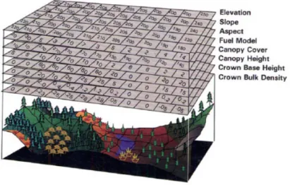
Figure 3-1. Raster landscape input layers required from the GIS for FARSITE simulation (Finney 1998).
At each of these points (vertices), fuel, topography and weather are acquired from the input data (Figure 3-1) and used to calculate fire behaviour and spread direction.
Raster files are created by interpolating the fire behaviour values from neighbour vertices, indicating Arrival Time, Fireline Intensity, Rate of Spread, Flame Length, Heat/Area, in any resolution (independent of landscape resolution).
The simulation process (figure 3-2) consists of:
1. Importing spatial data to create a landscape (.lcp) file;
2. Generating wind, weather, fuels moisture, and others file inputs, and with the landscape file create a project (.fpj) file
3. Initiating simulation
4. Setting simulation parameters, fire behaviour options, ignitions and selecting outputs
5. Run the simulation (start, stop, adjust, restart…) 6. Output interpretation.
FARSITE provides several outputs results from the simulation, as ASCII raster map of fire behaviour parameters, vector shape file contour, and ASCII string of values.
Optional GIS Themes Required
GIS Themes Build .lcp File
Initiate/Terminate
Optional ASCII inputs Required
ASCII Inputs Build .lcp File Save as
.fpj file Load Project
Set
Parameters DurationSet
Set Fire Behavior
Options
Set
Ignitions OutputsSet
Start/Restart
SIMULATION InterpretationSimulation
Save as .bmk file Load Bookmark Suspend/ Resume Export output files Optional GIS Themes Required
GIS Themes Build .lcp File
Initiate/Terminate
Optional ASCII inputs Required
ASCII Inputs Build .lcp File Save as
.fpj file Load Project
Set
Parameters DurationSet
Set Fire Behavior
Options
Set
Ignitions OutputsSet
Set
Parameters DurationSet
Set Fire Behavior
Options
Set
Ignitions OutputsSet
Start/Restart
SIMULATION InterpretationSimulation
Save as .bmk file Load Bookmark Suspend/ Resume Export output files
Figure 3-2. Plan of steps used to run a FARSITE simulation
3.3. Methodology
3.3.1. Applying the ModMed fire model to some historical fire data from Tapada de Mafra
On the 23rd August 1975, a large fire burned for three days, starting at 15:00. Each night the fire went out and re-ignited in the next day as the humidity fell.We assumed:
• We were modelling a surface level (litter and shrub layers) fire contagion, using horizontal continuity of the lower levels of vegetation for modelling the spread of fire.
• The moisture content would be similar across the whole landscape and the land use patterns for 1975 where the same as in 1974.
• Same average wind speed was used for the three days; wind direction was determined by the valley of the major water stream.
The simulation data and their preparation
• A map of the outline of the Tapada;
• An elevation map for the Tapada and surrounding area;
• A map showing 20 land use types for Mafra and surrounding area in 1974; • A map showing the outlines of the fire-affected area.
In each case, data were available for a rectangle which included the (non-rectangular) area of the Tapada. However, we only used data from within the Tapada because the estate is surrounded by a high wall which serves as an effective fire break. This unnatural situation helped to simplify the modelling.
The original maps were stored as shape files. They were imported to Idrisi to produce raster grid maps.
In each case, data were available for a rectangle which included the (non-rectangular) area of the Tapada. However, we only used data from within the Tapada because the estate is surrounded by a high wall which serves as an effective fire break. This unnatural situation helped to simplify the modelling. All the maps where clipped with the outline of Tapada de Mafra estate. The outline of the Tapada was held as a shape file (ArcView version 3.2). This was imported to Idrisi to produce a raster grid map in which the rasters inside the Tapada had the value '1' and those outside value '0'.
We use the following grid map specification for the Tapada area. The result is shown below. (figure 3-3) Bottom left: (97000,220000) Top right: (102000,2232000) Columns: 400 Rows: 240 Resolution: 12.5 m
Preparing the elevation grid map
The source file was stored as a shape file (ArcView version 3.2). We used the ArcView extension called 'Shape to DXF converter' to produce a DFX file. Next, we imported it to Idrisi32 to get an Idrisi vector file. This was rasterised onto a background image using the Idrisi 'LineRas' function. The background image was created using the Idrisi 'Initial' function.
Next, we used the Idrisi 'Intercon' function to build a raster surface from the rasterised lines. Finally, we used the Idrisi 'Window' function to cut out the area of interest, to produce an elevation grid map with the defined specifications. This was multiplied by the Tapada area grid (using Landlord 'Maptools'), to limit the data to the Tapada extent.
The resulting grid map was imported to Landlord 1.2 as shown in figure 3-4.
Figure 3-4. Digital elevation model (DEM) map of Tapada de Mafra area.
Preparing the land use grid map
The source file was again an ArcView 3.2 shape file. This was imported to Idrisi for Windows to produce an Idrisi vector file. This was rasterised using the Idrisi 'Polyras' function.
The conversion process had lost information about the meanings of the polygons (the land use classes associated with each area). These relationships were restored using a basic program which reclassified each raster value to the appropriate land use class. We added category names for each land use type by manual editing of the Idrisi image documentation file. Finally, we removed the information from outside the Tapada using the Landlord 'MapTools' to multiply a grid of the Tapada area (0 or 1) by the land use grid.
Figure 3-5. Land use map of Tapada de Mafra area.
Estimating the fuel horizontal continuity
We assumed that we were modelling fire contagion for surface fuels. The fire might affect the tree canopies, but the spread of the fire would be in litter and shrub layers. So we were only interested in the horizontal continuity of the lower levels of vegetation for modelling the spread of fire.
To translate the land use classes to horizontal fuel continuity values we prepared a table which contained estimates of fuel horizontal continuity for each land use type classes. Then we use a hand-made program to translate the land use classes to fuel horizontal continuity values. The resulting map is shown below (Figure 3-6).
Estimating the fuel moisture using riparian zones
We had an ArcView map of water courses in the Tapada, and rasterised this into Idrisi with values from 0 to 4, thus:
We then used the ModMed Seed Flow model to produce a more diffuse pattern. We used the linear diffusion pattern with a maximum range of 100 metres to give the map shown below.
Figure 3-7. Water lines map and fuel moisture estimation.
Estimating the fuel moisture using aspect
Another possible source of fuel moisture pattern is aspect. We produced an aspect grid using the Idrisi 'Surface' function (figure 3-8), and then used Landlord 'MapTools' to reorder the values to range from 1 for exactly south-facing and 3 for exactly north-facing.
These two approaches made it possible to generate possible maps of estimated fuel moisture content. After testing with several combinations, we decided to use a uniform map with all areas having a fuel moisture content of 10%.
Winds
From weather reports from nearby weather station (Sintra), we estimated the direction and speed of the mid-afternoon winds for the three fire days.
We discovered a bug in the model which reversed the direction of the wind effect. To work around this problem, we added 180 degrees to the direction which we really wanted, so 30° became 210° when entering the settings.
We set up a workspace using the ModMed Fire process model. The default settings were used, with wind information set to 7m/s wind speed and 210 degrees for wind direction
The damage maps
The damaged area map from the 1975 wildfire was imported to Idrisi from ArcView shape files to give binary raster grids (each raster is either damaged or undamaged). These damage maps show approximate areas of damage. The outlines were sketched by forest rangers onto paper maps. The pattern of actual damage (approximate) is shown in the map below.
3.3.2. Applying FARSITE using custom fuel models developed for Tapada de Mafra
The objective of the study were to determine the areas within Tapada de Mafra with a higher potential of summer fire hazard, enabling a subsequent test of diverse management strategies designed to minimize the consequences of a wildfire.
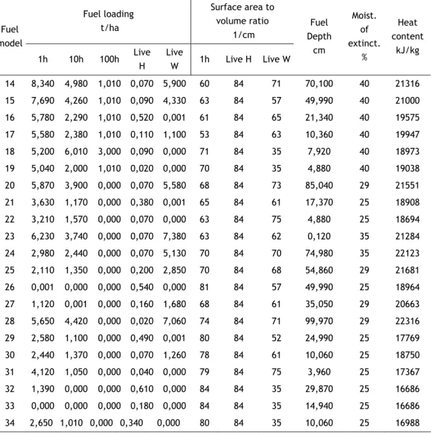
The existing Tapada de Mafra GIS was used to generate the raster themes: elevation, slope, aspect and fuel models. A field survey of the mapped vegetation patches (land use map of 1995) was carried (summer 2000), correcting their boundaries where necessary, and assigning custom fuel models developed with BEHAVE system (Burgan and Rothermel 1984). Data to develop the fuel models was obtained from indirect sampling procedures, namely line transects, and was subsequently used to estimate loading by fuel type, condition and size-class; published information was the source for the remaining fuel inputs. From this process result 21 custom fuel models (Table 3-1).
Table 3-1. Custom fuel models parameters (metric units) used in the FARSITE simulations
Fuel loading t/ha Surface area to volume ratio 1/cm Fuel model 1h 10h 100h Live H Live W 1h Live H Live W Fuel Depth cm Moist. of extinct. % Heat content kJ/kg 14 8,340 4,980 1,010 0,070 5,900 60 84 71 70,100 40 21316 15 7,690 4,260 1,010 0,090 4,330 63 84 57 49,990 40 21000 16 5,780 2,290 1,010 0,520 0,001 61 84 65 21,340 40 19575 17 5,580 2,380 1,010 0,110 1,100 53 84 63 10,360 40 19947 18 5,200 6,010 3,000 0,090 0,000 71 84 35 7,920 40 18973 19 5,040 2,000 1,010 0,020 0,000 70 84 35 4,880 40 19038 20 5,870 3,900 0,000 0,070 5,580 68 84 73 85,040 29 21551 21 3,630 1,170 0,000 0,380 0,001 65 84 61 17,370 25 18908 22 3,210 1,570 0,000 0,070 0,000 63 84 75 4,880 25 18694 23 6,230 3,740 0,000 0,070 7,380 63 84 62 0,120 35 21284 24 2,980 2,440 0,000 0,070 5,130 70 84 70 74,980 35 22123 25 2,110 1,350 0,000 0,200 2,850 70 84 68 54,860 29 21681 26 0,001 0,000 0,000 0,540 0,000 81 84 57 49,990 25 18964 27 1,120 0,001 0,000 0,160 1,680 68 84 61 35,050 29 20663 28 5,650 4,420 0,000 0,020 7,060 74 84 71 99,970 29 22316 29 2,580 1,100 0,000 0,490 0,001 80 84 52 24,990 25 17769 30 2,440 1,370 0,000 0,070 1,260 78 84 61 10,060 25 18750 31 4,120 1,050 0,000 0,040 0,000 79 84 75 3,960 25 17367 32 1,390 0,000 0,000 0,610 0,000 84 84 35 29,870 25 16686 33 0,000 0,000 0,000 0,180 0,000 84 84 35 14,940 25 16686 34 2,650 1,010 0,000 0,340 0,000 80 84 35 10,060 25 16988
The simulation data and their preparation
Landscape file
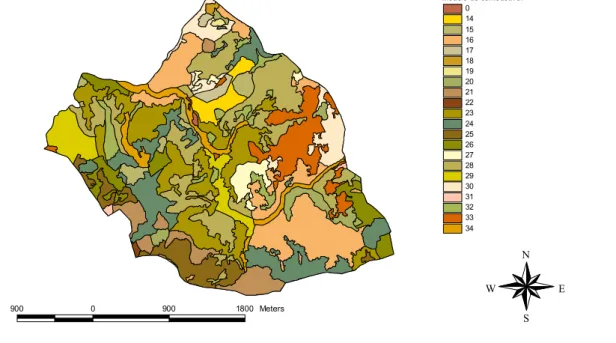
Theme maps where created in ArcView 3.2 using Spatial Analyst. Shape format maps where first converted in grid raster format, with a resolution of 10 meters. These grid maps had been exported as ASCII grid, to be used as inputs in FARSITE landscape. Landscape file was created with the required GIS themes for elevation, slope, aspect, fuel models and canopy cover. M o d e l o d e c o m b u s t í v e l 0 1 4 1 5 1 6 1 7 1 8 1 9 2 0 2 1 2 2 2 3 2 4 2 5 2 6 2 7 2 8 2 9 3 0 3 1 3 2 3 3 3 4 9 0 0 0 9 0 0 1 8 0 0 M e t e r s N E W S
Figure 3-10. . Fuel models map of Tapada de Mafra.
Weather, wind and fuel files
This initial approach uses weather data collected in a meteorological station located within the Tapada area, for the period of 10 to 17 July 2000, which should reflect an example of the typical summer situation.
Beside the custom fuel models information, FARSITE also requires stream data (space delimited ASCII format) for fuels moistures. This information is used to begin the process of calculating site specific fuel moistures at each time step during the simulation. Fuel moistures are specified for 1h, 10, 100h, live herbaceous and live wood fuels. For this simulation we used values of 8% for 1h fuel, 10% for 10h and 100h and 100% for live fuels, for a moderate weather scenario.
After some tests simulation duration was set to start 14/July at 14:00 and end 16/July at 22:00.
3.4. Results
3.4.1. Landlord fire simulation
We ran the simulation several times by setting fire to a small area around ignition point, and found that the model typically predicted a spread in a more westerly direction than actually happened. Either the predicted fire affected a very small area, or if it spread to the main area of high fuel continuity, it would burn a large area westward (uphill, with a following wind and good fuel availability). A typical result of a larger fire is shown in figure 3-11.
Figure 3-11. Example of an output map of the simulation.
The model typically predicted spread in a bigger area than it actually happened. A problem is the fact that we are not sure what, if any, fire-fighting actions were taken at the times of the fires: the eventual pattern of each fire may have been greatly affected by such interventions.
It seemed that the wind and topography could be considered to be 'driving' the spread of the fire, and the fuel properties were limiting the spread.
The wind directions which we used seem to be more easterly than indicated by the actual damage pattern. Perhaps the local topography either at Sintra (where the winds were measured) or at Mafra meant that the winds were actually rather different in the two places.
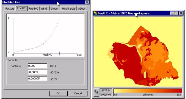
Figure 3-12. Fuel horizontal continuity (HC) model graphic and fuel HC map for Tapada de Mafra
The fuel horizontal continuity map which we estimated was no more than an educated guess. The default settings for the fire model make the contagion probability very sensitive to changes in fuel continuity between about 50 and 70 (figure 3-12) and the fire starting area in the simulations contained a mixture of fuel HC values ranging from 10 to 60 so it's quite likely that the fire patterns we simulated were too strongly influenced by the Fuel HC map.
3.4.2. FARSITE fire simulation
FARSITE simulation runs for a period of 2 days and 8 hours. Ignition point was located proximally to the buildings area, in the north-centre of Tapada.
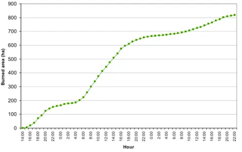
0 100 200 300 400 500 600 700 800 900 14 :0 0 16 :0 0 18 :0 0 20 :0 0 22 :0 0 0: 00 2: 00 4: 00 6: 00 8: 00 10 :0 0 12 :0 0 14 :0 0 16 :0 0 18 :0 0 20 :0 0 22 :0 0 0: 00 2: 00 4: 00 6: 00 8: 00 10 :0 0 12 :0 0 14 :0 0 16 :0 0 18 :0 0 20 :0 0 22 :0 0 Hour B u rn ed ar e a (h a)
Figure 3-14. Graphic evolution of Burned area versus Time, during the simulation.
Burned area, at the end of simulation, totalizes 818 ha. Is notorious the effect of changes in fire propagation during night time, resulting in a lower increase in the burning area (Figure 3-14). In most of the area fire from reach the outside wall during the simulation period.
Output maps
We test to export results of the simulation as ASCII raster maps. Fire line intensity, Rate of spread and Time of arrival had been imported to ArcView GIS and converted in grid format.
f i r e l i n e i n t e n s i t y ︵k W / m ︶0 - 5 0 0 5 0 0 - 2 0 0 0 2 0 0 0 - 4 0 0 0 4 0 0 0 - 1 0 0 0 0 > 1 0 0 0 0 N o D a t a 1 0 1 2 K i l o m e t e r s
The result show that most of the area burn with a low intensity fire (below 500 kW/m). Some areas with more intense fire behaviour where identified in this simulation.
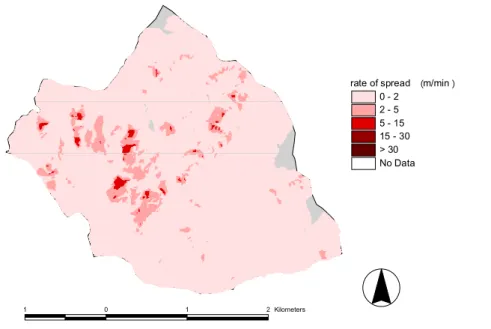
r a t e o f s p r e a d ︵ m / m i n ︶0 - 2 2 - 5 5 - 1 5 1 5 - 3 0 > 3 0 N o D a t a 1 0 1 2 K i l o m e t e r s
Figure 3-16. Rate of spread map, resulting from FARSITE simulation.
The resulting map for the rate of spread also show the location of some areas with faster fire spread, even if the simulation conditions where moderate.
3.5. Conclusions
Both programs are proven to work as simulators fire spread in the landscape. Landlord results were more limited, since it only simulates the potential damage area, i. e., the area potentially affected by fire. It is also less demanding in terms of inputs, which somehow is revealed in the results. The software was still in development when we tested. After the end of project ModMed no more improvement was made and at this time the software is not available.
FARSITE proved to be a program with greater capacity for simulation, producing a set of detailed results about the behavior of fire, not only in number of parameters but also in time and space detail. It is however far more demanding in information, especially in relation to meteorological variables. The quality of the results are dependent on the quality of inputs, and these variables, together with the availability of fuel models mapping may be a major limitation to effective implementation of the program. Training managers in the development of this information and in the analyses of simulation results can be an important issue in FARSITE wide application.