MPPT study from a solar photovoltaic panel according to perturbations induced by shadows

SCHOOL OF SCIENCE AND TECHNOLOGY

DEPARTMENT OF PHYSICS

MPPT study from a solar photovoltaic panel

according to perturbations induced by shadows

Ana Catarina das Neves Foles

Supervision: Mouhaydine Tlemçani, Ph.D.

Co-supervision: Paulo Manuel Ferrão Canhoto, Ph.D.

Masters in Solar Energy Engineering

Dissertation

UNIVERSITY OF ÉVORA

SCHOOL OF SCIENCE AND TECHNOLOGY

DEPARTMENT OF PHYSICS

MPPT study from a solar photovoltaic panel

according to perturbations induced by shadows

Ana Catarina das Neves Foles

Supervision: Mouhaydine Tlemçani, Ph.D.

Co-supervision: Paulo Manuel Ferrão Canhoto, Ph.D.

Masters in Solar Energy Engineering

Dissertation

i

Abstract

This work addresses the mathematical and physical modelling of photovoltaic cells and modules, in order to obtain the maximum power output under different environmental operation conditions, including the effect of shadow. Firstly, the Bisection, Newton-Raphson and Secant methods were evaluated for obtaining the characteristic curve of photovoltaic cells, based on the single diode five parameters model and using the values of ideal parameters. Subsequently, the Nelder and Mead algorithm was used to determine the five parameters of the model by fitting the characteristic curve to current and voltage measurements, and accounting to the dependence of cell temperature on environmental conditions by coupling this method to a thermal model of the module. Finally, partial shadowing of photovoltaic modules was studied through a laboratorial experiment, to which conditions the MPPT is calculated through the polynomial fitting of power-voltage curve.

Keywords

iii

Resumo

Estudo do MPPT de um painel fotovoltaico em função de perturbações induzidas por sombras

Este trabalho consiste na modelação física e matemática de células e módulos fotovoltaicos, com o intuito de obter a sua máxima potência sob diferentes condições de operação, incluído o efeito de sombreamento. Primeiramente, os métodos da Bisecção, Newton-Raphson e Secante foram avaliados recorrendo ao modelo de um díodo e cinco parâmetros de forma a obter a curva característica das células fotovoltaicas, com valores de parâmetros ideais. Seguidamente, o algoritmo de Nelder e Mead foi utilizado para determinar os cinco parâmetros do modelo, recorrendo ao ajuste da curva característica com medidas experimentais de corrente e tensão, e a dependência que os parâmetros ambientais têm na obtenção da temperatura da célula, através do acoplamento do algoritmo com um modelo térmico do módulo. Finalmente, foi estudado o sombreamento parcial de módulos fotovoltaicos através de uma experiência laboratorial, na qual o MPPT é calculado por um ajuste de um polinómio à curva potência-tensão.

Palavras-chave

v

Acknowledgements

This page is devoted to express my gratitude to the people who made this work possible. Firstly, I would like to thank the two pillars who guided me on this journey and who always tryed to put me on the right path. I would like to express my appreciation to my supervisor, Professor Mouhaydine Tlemçani, for all the support he gave me in the realization of this work, availability, sharing of knowledge and ideas, keeping my motivation high, giving me good advices, providing me opportunities for the work to advance, and the good person he went during this work. I want to thank to my co-supervisor, Professor Paulo Canhoto, for being more than a co-supervisor, for sharing his knowledge, being patient and always trying to understand my doubts, giving me a lot of good advices, and the opportunity to appreciate the good person he is.

I want to express my gratitude to Professor Mourad Bezzeghoud for giving me the opportunity to go to the AMPSECA Conference 2017, in Agadir, Morocco.

I am grateful to Instituto de Ciências da Terra (ICT) of the University of Évora for the provided materials, which made possible the realization of the laboratory experiments. To my group of colleagues, my teacher and colleague André Albino, who have always been available to help me and share his knowledge, and to my colleagues Md Tofael Ahmed and Masud Rana Rashel for their fellowship and help.

I wish to express my gratitude to my parents, Rui Foles and Fernanda Foles, for the sacrifice made correspondent to my entire cycle of studies, and for giving me all the support for the accomplishment of this work, helping me keeping motivated through the entire process. Finally, I wish to express my gratitude to my syster and my brother, Rita e Ricardo, to my boyfriend, Dorin, and to all my friends for the excellent people they are to me, allowing me to don’t be afraid of being audacious and for making me a better person each day.

vii

Contents

Chapter 1 - Introduction ... 1

1.4 State of the art ... 5

1.4.1 Solar cell modelling and simulation ... 8

1.4.2 Parameters determination and sensitivity analysis ... 9

1.4.3 Impact of shadow on the power output of photovoltaic cells ... 9

1.5 Structure of the dissertation ... 11

1.6 Notation ... 11

Chapter 2 – Photovoltaic cell modelling ... 13

2.1 Mathematical model formulation ... 13

2.1.1 Single diode model ... 14

2.1.2 Single diode detailed model ... 15

2.1.3 Double diode model ... 16

2.1.4 Considerations on photovoltaic cell models ... 16

2.2 Determination of the characteristic current-voltage curve... 18

2.2.1 Bisection method (Binary-Search or Bolzano) ... 19

2.2.2 Secant method ... 20

2.2.3 Newton-Raphson method ... 21

2.3 Application results ... 22

2.3.1 Bisection method ... 22

2.3.2 Secant method ... 23

viii

2.4 Coupling Bisection and Newton-Raphson methods ... 25

2.4.1 Application results ... 26

Chapter 3 - Parameters determination using the Nelder and Mead

algorithm ... 28

3.1 Determination of the parameters of a module ... 28

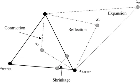
3.1.1 The Nelder and Mead algorithm ... 29

3.2 Determination of guess values of the parameters for the initial simplex ... 35

3.3 Application of the Nelder and Mead for the five parameters model based on the available data of a module ... 37

3.3.1 Initial simplex numerical tolerance ... 39

3.3.2 Imposed noise from the initial curve ... 40

3.3.3 Cycle tolerance and stopping criterion ... 41

3.4 Considerations ... 42

Chapter 4 - Nelder and Mead algorithm development and experimental

validation ... 43

4.1 Materials and methods ... 43

4.1.1 Data acquisition system ... 44

4.1.2 Function Generator and GPIB devices ... 45

4.1.3 Photovoltaic module and artificial source ... 45

4.1.4 Instrumentation for air temperature and wind speed measurement ... 46

4.1.5 Temperature sensor with digital display ... 46

4.2 Integrated algorithm for determination of cell temperature, model parameters and maximum power output ... 47

4.2.1 Estimation of cell temperature based on measurements ... 48

4.2.2 Thermal model of the photovoltaic module and cell temperature determination ... 48

ix

4.4 Considerations ... 55

Chapter 5 - MPPT estimation under shadow conditions ... 57

5.1 The concept of shadow and its effects on photovoltaic conversion of a module 57 5.2 Analysis of characteristic curve under shaded and unshaded conditions ... 58

5.2.1 Materials and methods ... 58

5.2.2 Module 1 and Module 2 in unshaded conditions ... 58

5.2.3 Module 1 and Module 2 under shaded conditions ... 61

5.3 Curve fitting through polynomials ... 65

5.4 Considerations ... 67

Chapter 6 - Conclusions and future work ... 69

Chapter 7 - References ... 71

xi

List of figures

Chapter 1

Figure 1.1.1 - Global horizontal irradiation distribution [𝑘𝑊ℎ/𝑚2] [6]. ... 2

Figure 1.3.1 - World energy consumption prediction until 2040 [2]. ... 4

Figure 1.4.1 - Illustration of N-type and P-type semiconductors. (a) n-type, with excess of electrons. (b) p-type, with excess of positive holes [7]. ... 5

Figure 1.4.2 - Illustration of the photovoltaic materials chart [1]. ... 6

Chapter 2

Figure 2.2.2 – Equivalent circuit of single diode model considering both the shunt and series resistances. ... 15

Figure 2.2.3 – Equivalent circuit of the double diode model. ... 16

Figure 2.2.4 – I-V and P-V curves representation, with the relevant current and voltage values. ... 17

Figure 2.3.1 - Bisection method schematic illustration. Adapted from [18]. ... 19

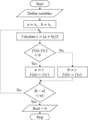
Figure 2.3.2 – Bisection method algorithm flowchart. ... 19

Figure 2.3.3 - Secant method schematic illustration. Adapted from [18]. ... 20

Figure 2.3.4 - Secant method algorithm flowchart. ... 20

Figure 2.3.5 - Newton-Raphson method schematic illustration. Adapted from [18]. ... 21

Figure 2.3.6 - Newton-Raphson algorithm flowchart. ... 22

Figure 2.4.1 - Error of Bisection method cycle, as a function of the number of iterations. ... 23

Figure 2.5.1 – Flowchart for coupling Bisection and Newton Raphson methods. ... 26

Figure 2.5.2 - Results of I-V and P-V curves of the coupling method. ... 27

Chapter 3

xii

Figure 3.1.3 - Flowchart of the Nelder and Mead algorithm. ... 33

Figure 3.1.4 - Stopping criterion illustration, with a three vertices example. ... 35

Figure 3.2.1 - Error function vs. Irradiance [W/m2_{] [26]. ... 36}

Figure 3.2.2 - Error function vs. Cell temperature [K] [26]. ... 36

Figure 3.2.3 - Error function vs. diode ideality factor [26]. ... 36

Figure 3.2.4 – Error function vs. shunt resistance [Ω] [26]... 36

Figure 3.2.5 - Error function vs. diode saturation current [A] [26]. ... 36

Figure 3.3.1 – Relative difference between the obtained values with the Nelder and Mead algorithm and NREL values as a function of the initial simplex maximum deviation. ... 39

Figure 3.3.3 - Difference between Nelder and Mead results and NREL values, as a function of the noise in the current measurements. ... 40

Figure 3.3.4 - Difference between Nelder and Mead results and NREL values, as a function of the tolerance. ... 41

Chapter 4

Figure 4.2.1 – Flowchart of the algorithm for the determination of cell temperature, model parameters and power output at MPP. ... 47

Figure 4.2.2 - Cost function as a function of the variation of the cell temperature. ... 48

Figure 4.2.3 - Energy balance of a solar photovoltaic module. Adapted from [46]. ... 49

Figure 4.2.4 - Thermal network of the solar photovoltaic module studied model, considering convection, radiation and conduction losses. ... 51

Chapter 5

Figure 5.2.2 - P-V curve of Module 1, measured under normal irradiation conditions. ... 59

Figure 5.2.3 - I-V curve of Module 1, measured under normal irradiation conditions. ... 60

Figure 5.2.4 - Module 2 measured P-V curve under normal irradiation conditions. ... 60

xiii

Figure 5.2.6 - Module 1 and Module 2 shaded cells experimental configurations – Cases of

shadow 1 and 2. ... 61

Figure 5.2.7 - I-V curve of the Module 1, case of shadow 1. ... 62

Figure 5.2.8 - P-V curve of the Module 1, case of shadow 1. ... 62

Figure 5.2.9 - I-V curve of the Module 1, case of shadow 2. ... 62

Figure 5.2.10 - I-V curve of the Module 1, case of shadow 2. ... 63

Figure 5.2.11 - I-V curve of module 2, case of shadow 1. ... 63

Figure 5.2.12 - P-V curve of module 2, case of shadow 1. ... 64

Figure 5.2.13 - I-V curve of module 2, case of shadow 2. ... 64

Figure 5.2.14 - P-V curve of module 2, case of shadow 2. ... 64

Figure 5.3.1 - Fifth polynomial fitting with the P-V curve of module 1, case of shadow 1. ... 66

Figure 5.3.2 - Fifth polynomial fitting with the P-V curve of module 1, case of shadow 2. ... 66

Figure 5.3.3 - Eighth polynomial fitting with the P-V curve of module 2, case of shadow 1. ... 67

xv

List of tables

Chapter 2

Table 2.4.1 - Parameters ideal values. ... 22

Table 2.4.2 – Secant application results. ... 24

Table 2.4.3 - Newton-Raphson application results. ... 25

Table 2.5.1 – Results with coupled methods. ... 27

Chapter 3

Table 3.3.1 – Characteristics of the module Sunrise Solartech SR-M654225 [37]. ... 37

Table 3.3.2 - Standard coefficients of the Nelder and Mead algorithm [20]. ... 38

Table 3.3.3 – Reference parameters for the Sunrise Solartech SR-M654225 module [37]. ... 38

Chapter 4

Table 4.2.1 - Initial conditions of the integrated algorithm. ... 55

Table 4.2.2 – Results of the estimation of the temperatures, five parameters and maximum power. ... 55

Chapter 5

xvii

Nomenclature

Simbol Description Unit

𝐴_𝑐 Area of one cell [𝑚2]

𝐴𝑚 Area of the module [𝑚2]

𝐴_𝑟 Half of the laboratorial wall area [𝑚2]

𝑎, 𝑎_𝑘, 𝑎 _𝑘+1 Value of parameter 𝑎 during iterative process − 𝑏, 𝑏𝑘, 𝑏 𝑘+1 Value of parameter 𝑏 during iterative process −

𝐶_𝑛 Curve coefficients −

𝑒_𝑖 Bases of a vector −

𝑒𝑘 Errors associated with a succession of values −

𝐸(𝐼) Error function value −

𝑓_𝑏 Objective function value of the highest vertex −

𝑓𝑤 Objective function value of the lowest vertex −

𝐺𝑟 Number of Grashof −

𝐺_𝑡 Irradiance [𝑊/𝑚2]

ℎ𝑐𝑜𝑛𝑑,𝑏 Conduction heat transfer coefficient of backsheet [𝑊/𝑚2𝐾]

ℎ_{𝑐𝑜𝑛𝑑,𝑔} Conduction heat transfer coefficient of glass [𝑊/𝑚2𝐾] ℎ𝑐𝑜𝑛𝑣,𝑏−𝑎 Convection heat transfer coefficient from backsheet to air [𝑊/𝑚2𝐾]

ℎ_{𝑐𝑜𝑛𝑣,𝑔−𝑎} Convection heat transfer coefficient from glass to air [𝑊/𝑚2𝐾] ℎ𝑟𝑎𝑑,𝑏−𝑎 Radiation heat transfer coefficient from backsheet to air [𝑊/𝑚2𝐾]

ℎ_{𝑟𝑎𝑑,𝑔−𝑎} Radiation heat transfer coefficient from glass to air [𝑊/𝑚2𝐾]

𝐼 Net current [𝐴]

𝐼_𝐷 Current in the diode [𝐴]

𝐼𝑒𝑟𝑟 Current output with error [𝐴]

𝐼𝑚𝑝 Maximum power point current [𝐴]

𝐼_𝑝ℎ Photo-generated current of the cell [𝐴]

𝐼𝑠 Reverse saturation current of the cell [𝐴]

𝐼𝑠𝑐 Short circuit current [𝐴]

𝐼_𝑠𝑡𝑑 Current standard output [𝐴]

𝐼𝑠1 Dark saturation current of the first diode modelling the

diffusion current component of the cell [𝐴]

𝐼_𝑠2 Dark saturation current of the second diode modelling the

recombination in the space charge region of the cell [𝐴]

xviii

𝐼_(𝑝̂)𝑖 Estimated current value [𝐴]

𝑘 Boltzmann’s gas constant [𝐽/𝐾]

𝑘𝑎𝑖𝑟 Thermal conductivity of the air [𝑊/𝑚𝐾]

𝑘_𝑏 Thermal conductivity of the backsheet [𝑊/𝑚𝐾]

𝑘_𝑔 Thermal conductivity of the glass [𝑊/𝑚𝐾]

𝐿 Length of the module [𝑚]

𝑛 Diode ideality factor of the cell −

𝑛𝑏 Number of bits −

𝑛_𝑠 Number of series connected cells in the module −

𝑁_𝑐 Number of cells in the module −

𝑃_𝑚𝑝 Maximum power output [𝑊]

𝑃𝑟 Prandtl number −

𝑞 Electronic charge [𝐶]

𝑄𝑏𝑜𝑡𝑡𝑜𝑚 Total heat loss of the module, from the cell to the backsheet [𝑊]

𝑄𝑡𝑜𝑝 Total heat loss of the module, from the cells to the glass [𝑊]

𝑅𝑎 Rayleigh number −

𝑅𝑐𝑜𝑛𝑑𝑢𝑐𝑡𝑖𝑜𝑛 Thermal resistance for conduction heat transfer [𝑚2𝐾/𝑊]

𝑅_{𝑐𝑜𝑛𝑣𝑒𝑐𝑡𝑖𝑜𝑛} Thermal resistance for convection heat transfer [𝑚2𝐾/𝑊] 𝑅_{𝑒𝑞𝑢𝑖𝑣𝑎𝑙𝑒𝑛𝑡} Thermal resistance for the equivalent heat transfer [𝑚2𝐾/𝑊] 𝑅𝑟𝑎𝑑𝑖𝑎𝑡𝑖𝑜𝑛 Thermal resistance for radiation heat transfer [𝑚2𝐾/𝑊]

𝑅_𝑠 Internal series resistance of the cell [Ω]

𝑅_𝑠ℎ Shunt resistance of the cell [Ω]

𝑆 Interval −

𝑆𝑓 Objective function −

𝑆_𝑘 Subinterval −

𝑇_𝑎 Temperature of the ambient air [𝐾]

𝑇𝑏 Temperature of the backsheet [𝐾]

𝑇_𝑐 Temperature of the cell [𝐾]

𝑇_{𝑓𝑖𝑙𝑚𝑏−𝑎} Average temperature between the backsheet and the air [𝐾] 𝑇_{𝑓𝑖𝑙𝑚𝑔−𝑎} Average temperature between the glass and the air [𝐾]

𝑇𝑔 Temperature of the glass of the module [𝐾]

𝑈_𝐿 Overall heat transfer coefficient [𝑊/𝑚2𝐾]

xix

Greek symbols

𝛼 Reflection coefficient −

𝛼𝑠 Silicon absorptivity −

𝛽 Volumetric expansion coefficient [𝐾−1]

𝛾 Expansion coefficient −

𝜀𝑏 Backsheet emissivity −

𝜀_𝑔 Glass emissivity −

𝜀𝑟 Laboratory room combined emissivity −

𝜂_𝑒 Electric power efficiency [%]

𝜌 Contraction coefficient − 𝜎 Shrinkage coefficient − 𝜎𝑏 Stefan-Boltzmann constant [𝑊/𝑚2𝐾4] 𝜏 Glass transmissivity − ∆𝑥𝑏 Backsheet thickness [𝑚] ∆𝑥𝑔 Glass thickness [𝑚]

𝑣_𝑐 Kinetic viscosity of air [𝑚2/𝑠]

𝑉 Voltage imposed across the cell [𝑉]

𝑉𝑚𝑝 Maximum power point voltage [𝑉]

𝑉_𝑜𝑐 Open circuit voltage [𝑉]

𝑉𝑡 P-n junction thermal voltage [𝑉]

𝑥_𝐶 Simplex vector where function gets the contracted value − 𝑥_𝐸 Simplex vector where function gets the expanded value − 𝑥𝑘 Secant and Newton-Raphson methods initial condition −

𝑥_𝑘+1 Bisection, Secant and Newton-Raphson iterations values −

𝑥_𝑘−1 Secant method initial condition value −

𝑥𝑚𝑖𝑛 Vertix who corresponds to the lowest function value −

𝑥_𝑚𝑎𝑥 Vertix who corresponds to the highest function value − 𝑥_𝑅 Simplex vertix where function gets the reflected value −

𝑥₀ Centroid of all vertices, except the highest value vertex

calculated in the function −

xx

Acronyms list

AC Alternating current. DAQ Data acquisition board.

DC Direct current.

GPIB General-Purpose Interface of Bus.

MPP Maximum power point.

MPPT Maximum power point tracking. NOCT Nominal Operating Cell Temperature. NREL National Renewable Energy Laboratory.

SAM System Advisor Model.

STC Standard Test Conditions. USB Universal Serial Bus.

List of communications

This work lead to the realization of three oral contributions. The first contribution was related to the first part of this work, which corresponded to the photovoltaic cell modelling, and happened in the University of Évora, in the WES Conference, organized by the Instituto de Ciências da Terra (ICT) (1). The second part of this work, which is related with the five parameters determination based on the one diode model, was presented in the AMPSECA Conference 2017, which took place in Agadir, Morocco (2), and also in the Workshop “Como fazer um artigo cientíco?”, organized by the ECT, presented in the University of Évora (3).

(1) Foles, A. Albino e M. Tlemçani, “Convergence speed optimization of iterative methods for a Photovoltaic Cell simulation”, in WES Conference, University of Évora, Portugal, 2016.

(2) C. Foles, A. Albino e M. Tlemçani, “Real time characterization of a photovoltaic panel using the five parameters model,” em AMPSECA 2017, Agadir, Morocco, 2017.

(3) C. Foles, A. M. Tlemçani. “Real time characterization of a photovoltaic module considering the single diode five parameters model”, em “Workshop: Como fazer um artigo cientifico?”, ECT of the University of Évora, Portugal, 2017.

1

1 Chapter 1 - Introduction

Current chapter is devoted to a photovoltaic energy overview. The technology state of the art is presented, in order to gather all the literature research made related to this matter. This dissertation main objectives and motivations will be discussed, so the reader can understand the core of this work.

1.1 Framework

The impact of electricity expansion was a growing technology, economic and social activities development, from which an extreme dependency on electricity was born. Electricity is currently a utility, and this fact has caused quite a lot of discussion in the recent decades, due to the consequences of its generalized use and mass exploitation of the primary energy resources used for its generation. Energy supply is currently one of the biggest problems that the human development is facing as the world’s electricity production is based mainly in the fossil fuels exploitation and the energy consumption is increasing [1, 2]. The intensive use of fossil fuels leads to large greenhouse gases emissions, and thus to a global warming increase, which has consequences such as average sea level increase, extinction of animals and plants and changes on the intensity of rain. In response to this problem, renewable energies technologies have arisen, powered by renewable sources, as the solar energy, wind, biomass and biofuels and sea waves and tides.

The energy could be harnessed to produce electricity [3]. Photovoltaic conversion is one of the most promising technologies, due to the uniform world availability of the solar resource

Introduction

Chapter 1

-

Introducti

on

2

and to the direct conversion into electric energy [4]. The total worldwide installed capacity of the photovoltaic technology was by the end of 2015 an amounted value of 227.1 GW. Also in 2015, the world’s installed photovoltaic capacity reached 50 GW [5]. It is expected that solar photovoltaic will become a serious alternative to fossil fuels in the nearest future. The issues concerning the energy independence, energy security, stability of energy supply and energy sources diversification will become crucial these days [3]. Photovoltaic systems, except for the concentration systems, have the advantage of using not only direct sunlight but also the diffuse component of sunlight, i.e. solar photovoltaic technology produces power even if the sky is not completely clear, which could enable the photovoltaic effective deployment in all the world regions [5]. World irradiation distribution is shown in Figure 1.1.1.

Figure 1.1.1 - Global horizontal irradiation distribution [𝑘𝑊ℎ/𝑚2] [6].

A solar photovoltaic system is constituted by photovoltaic modules, which are composed of several individual cells electrically connected between each other, and convert solar energy directly into electricity [7].

On one hand, photovoltaic energy generation strongly depends on the atmospheric conditions, via the incident solar irradiance and cell temperature and, on the other hand, there is only one operation point corresponding to the maximum power output [8]. Thus, a maximum power point tracker (MPPT), which makes use of a control circuit or logic that searches for this point, allows the extraction of the maximum power that the module can deliver under each operation conditions. The MPPT is a crucial procedure that deals with those changing

3

atmospheric conditions [9]. This strategy enables an optimization of the operating voltage to maximize the current [7]. MPPT are most applied in on-grid systems, to optimize the produced energy from the photovoltaic system. A high efficiency DC/DC converter functions as an optimal electrical load for a solar photovoltaic module, converting the power to a voltage or current more suitable than the load connected to these systems. Currently, MPPT cost has been reduced and its use is becoming more common [7].

In general, despite of the scientific and technological improvements and governmental incentives in some countries, the cost of the grid-connected energy is still high and yet not competitive with the fossil fuelled power plants [4].

1.2 Objectives

Present dissertation has the main aim of study the effect that some internal and external conditions have in the maximum power point tracking, in solar photovoltaic conversion systems. The construction of physical and mathematical models that simulate those conditions has motivated the world’s research with multiple diversified approaches.

Therefore, the aim of this study is divided in three main objectives, being the first the elaboration and validation of the single-diode mathematical model applied to the photovoltaic response characterization, by using numerical iterative methods. Three numerical iterative methods will be studied and compared. This approach has the aim of enabling the estimation of photovoltaic energy generation in a reliable and fast way.

The second objective is the estimation of the five parameters of the single diode model equivalent circuit of the photovoltaic cell. The determination of the parameters is made through the application of an existing and quite robust method, known as the Nelder and Mead algorithm, to a photovoltaic cell and module.

The third and final objective is to estimate the maximum power output of photovoltaics modules in shadow conditions, through a laboratorial procedure.

1.3 Motivation

Energy is one of the most crucial factors of economic development and prosperity of countries and society [10]. Growing energy demand is one of the key issues of the 21st century [10]. In

4

[2]is predicted that the world energy consumption will increase 28% between 2015 and 2040, as can be seen in Figure 1.3.1.

Figure 1.3.1 - World energy consumption prediction until 2040 [2].

Actual global energy situation is dominated by fossil fuels, which has severe impacts on regional climatic conditions and energy security, and nuclear power plants are directly related with radioactive emissions. The renewable energy technology is more secure, available and pollute less as compared with the conventional sources [10]. Photovoltaic systems provide multiple benefits, such as the fact of being non-polluting devices, needing of few maintenance, long lifetime and in some situations, the technology aloe the decentralised generation of energy [4].

Currently, photovoltaic technology development is divided in two key specific areas, with the main aim of increasing the overall conversion efficiency [9]:

 Cell material;

 Power conditioner technology (DC/DC and/or DC/AC converters).

Research is being carried out to advance in the solar cells materials area, such as monocrystalline and polycrystalline silicon cells, amorphous silicon and thin film cells, although their energy conversion efficiency is still low and their cost high [9, 4]. In the case of the power conditioner, the author of [9] defines it as having a very important role in the improvement of power conversion efficiency, and as being a good path to reduce the costs of photovoltaic systems.

5

The goal of maximizing the power output could be made with the help of power electronics, taking into consideration the variation of the environmental conditions. Optimal operating conditions guarantee is very important to minimize power loses, due to, for example, shadows, dust, debris or dirt accumulations, or system failures. The exploitation of robust algorithms applied to photovoltaic systems is a solution that guarantees achieving the maximum power point output, aiming the development of low cost converters, which is the main motivation of this dissertation.

1.4 State of the art

Alexandre Edmond Becquerel discovered the photovoltaic effect in 1839 through exposing selenium material to light, creating voltage across the material. In the following years, the scientists Charles Fritz, Edward Weston, Nikola Tesla and Albert Einstein contributed to the development of this effect [11]. The first application of solar photovoltaic cells was in space, in the year of 1958, where the cost isn’t an obstacle [7].

Photovoltaic cells are made of semiconductors, which are average conductors of electricity [7]. Having two semiconductors materials, if one of them is doped and has an excessive of electrons, its called the N-type semiconductor, and the other, which has lack of electrons, its called the type semiconductor, as can be observed in Figure 1.4.1, shown below. In the P-N region of a silicon type cell, the free electrons of the P-N-type silicon occupy the holes of the P-type silicon structure, creating an electrical field. The photons hit the cell and collide with the electrons of the silicon. Due to the electric field created by the P-N junction, the electrons flow from the P-film to the N-film by an electric conductor, generating electricity [7].

Figure 1.4.1 - Illustration of N-type and P-type semiconductors. (a) n-type, with excess of

6

The most commonly used materials in the solar cells fabrication are the monocrystalline and polycrystalline silicon (Si), cadmium telluride (CdTe), gallium arsenide (GaAs), and triple-junction solar cells, composed of indium gallium phosphide (InGaP) [12].

The cells are commonly divided in first, second and third generation. First generation cells are composed by monocrystalline and polycrystalline cells, which dominate the market on a 90% share, due to its higher efficiency and reliability compared to the other cells technologies [12]. Monocrystalline silicon is characterized by having a more intense process of production (by the Czochralski method, Cz), being more efficient, near 16%, and having a higher cost than the polycrystalline cells, which has an efficiency of 11%. Second generation has approximately a 10% share of the market and its related to the thin films deposition on rigids substrates. Its also characterized by using reduced materials and low energy consumption in the fabrication phase. The amorphous silicon is produced in vacuum through thin films deposition technology, and because the material is unstable its efficiency is about 6%. CIS (CuInSe2) have an efficiency of 11%, although face some problems in the fabrication phase.

Cadmium telluride (CdTe) cells have low production costs and its efficiencies are near 11%, however these elements are related to issues of contamination and scarcity. Finally, the third-generation cells are still in development, but are already being used in high solar concentration applications. Gallium arsenide (GaAs) is applied in high efficiency cells, reaching nearly 40%, and have a high cost. Tandem cells are used in high solar concentration, combined with Fresnel lenses, with multijunction cells. Organic cells are cells who are composed of organic semiconductors materials, and can set over flexible plastics and films, and could be transparent or have distinct colours (5% efficiency). Materials such as photonics are nanostructured materials who can be introduced in cells, to help in the solar radiation absorption, to increase the respective efficiency [1, 3, 7, 12]. Figure 1.4.2 presents a photovoltaic materials flowchart.

7

Because the cells size is very small, which corresponds to a small power production, solar cells are electrically connected, until the obtained power is the required for the desired application [10]. The degree of purity of the silicon needed to make a photovoltaic cell is high, compared with other electronic devices who use silicon as a component. This is one of the main reasons of the relative high cost of the modules and why electricity from solar photovoltaic systems is more expensive than electricity produced through fossil fuels [12]. However, the decreasing cells price over the past years have been contributing to its world spreading. Their expected lifetime had also increased, until 25 years or more [13]. Currently, research has been focused in developing the materials technology [12].

Photovoltaic systems could be grid-connected with the power grid or off-grid (stand-alone), which means that the installation is independent from the grid. Photovoltaic modules and an inverter, which converts the direct current in alternated current, in conditions of frequency, amplitude and phase of the grid, to inject in the electric grid, constitute the grid-connected systems. Off-grid photovoltaic systems are composed of photovoltaic modules, an inverter, a battery bank and a voltage regulator. Off-grid systems are mainly used in rural areas, far from the grid and where a decentralised energy generation is imposed [7].

Photovoltaic systems are also divided in two subcategories, depending on the existence or not of tracking. In this way, the photovoltaic system could be fixed, and usually facing to the south direction (local meridian), or could have a tracking system, which means that the photovoltaic modules follow the apparent sun trajectory in the sky, and this one could have a single (N-S or E-W) or double axis tracking (N-S and E-W) [10].

Photovoltaic conversion of solar energy has multiple applications such as building integrated photovoltaic (BIPV), transportation, communications, solar roadways, rural electrifications [10], illumination, water pumping, storage charging, desalinization, technologies hibridization and high concentration photovoltaics [7].

DC (direct current) electricity generated through photovoltaic systems can be converted in AC (alternated current) or stored in a battery bank for later use. Technology has supported the growth of renewable energies harvesting. Electronic converters made possible the connection between renewables energy systems and the existing power grid and conventional power plants, improving the energy harvesting through dedicated controls. Photovoltaic systems that are connected to the grid have a power electronics DC/DC converter to ensure the maximum power output with the MPPT, and a DC/AC converter to connect with the grid [13].

8

In [13] it is showed that the currently research challenges and opportunities are focused in reliability issues of the technology for power generation, medium voltage photovoltaic systems, high-efficiency thin-film cells and electric energy storage from photovoltaic systems. Until 2025 it is expected an improvement and implementation of high voltage photovoltaic systems, to increase its lifetime to 20-30 years and of its inverter, the implementation of micro-inverters, and the reduction of the levelized cost of electricity (LCOE) [13].

The possibility of predicting the response of a photovoltaic power plant due to the variation of incident irradiance, air temperature and load conditions is very important for sizing such systems and converters, as well as for the designing of the MPPT and control strategies [7].

1.4.1 Solar cell modelling and simulation

With the aim of extracting the maximum power from a photovoltaic plant, and with the help of MPPT control techniques, it is crucial to characterize study and model a single photovoltaic cell [14]. A solar cell can be described through an equivalent circuit, with the most used models being the single diode model and the double diode model, which are represented by four or five parameters, as described in [4, 7, 15, 16]. Those models allow the construction of the current-voltage curve (I-V) and of the power-voltage curve (P-V) [7]. These two models are widely known and differ from each other in terms of complexity and their use depends on the type of the application [4, 17]. Since the net electric current of the equivalent circuit is a transcendent function, it is necessary to use iterative methods, in order to obtain the solar cell current-voltage characteristic curve [7, 4]. This fact leads to a deeper study of root-finding iterative methods described in [18], and its application to the photovoltaic cell and module. Some of the numerical methods used for the construction of the I-V and P-V curves are the Bisection method, Newton-Raphson method and Secant method, as explained and presented in the work developed in [19].

The unknown parameters of the solar cell models must be determined for the given type of cell, whose characteristics are to be reproduced by the model. Several approaches for parameters determination can be adopted using the datasheet parameters or measured I-V curves [4].

9

1.4.2 Parameters determination and sensitivity analysis

A solar photovoltaic cell can be described by some points of the characteristic curve, such as the short circuit current, the open circuit voltage and the diode ideality factor [14]. Additionally to those values, the I-V curve could be described by four parameters, including the diode ideality factor, 𝑛: the reverse saturation current of the diode, 𝐼s, the photo-generated

current, 𝐼_𝑝ℎ, and the series resistance, 𝑅_𝑠. The shunt resistance, 𝑅_𝑠ℎ, is the fifth parameter of the detailed single diode model [4].

Nowadays, these parameters are not available directly from the manufacturers of photovoltaic modules. However, even if they were available from the manufacturers, the parameters of the model vary in time and with the aging of materials or technical faults. This is the main reason to identify these parameters by direct I-V measurements, in real-time [17].

A refined method is needed, in order to obtain a good photovoltaic cell or module characterization. A well-considered choice is to work with the Nelder and Mead algorithm [20], which is a direct search optimization method. In [20, 21, 22, 23] this method is explained and deeply analysed, and its application in the photovoltaic field is presented in [17, 24]. Nelder and Mead algorithm is widely applied to real problems, due to its robustness characteristic in solving optimization problems [24].

In [22] it is explained that the algorithm can converge to local minimums or maximums, although showing a good effectiveness after a few iterations steps. Another important aspect is its performance decreasing with the increase in the number of the parameters [24].

To well estimate the parameters using the Nelder and Mead algorithm it is crucial to understand the parameters response, becoming crucial to make a sensitivity parameters analysis, work developed by the research work in [25, 26].

The analysis of the Nelder and Mead algorithm was study and developed, leading to the presentation of the work in the AMPSECA Conference [27] and in the Workshop of ECT event [28].

1.4.3 Impact of shadow on the power output of photovoltaic cells

A shadow could be described as a “darker” region that is formed due to the obstruction of direct irradiance from the sun, caused by the existence of an obstacle between the source of light and shaded space. The shadow changes position according to the origin of light (sun),

10

and because of that, it varies in time, with environmental conditions and its geometric shape is not constant over time.

The shading of a photovoltaic module is a phenomenon that derives from the module-sun position and the surroundings obstacles. This could happen in any outdoor environment, being that surrounding ambient constituted by trees, passing clouds, high edification [29]. Shadow effect reduces the power output from photovoltaic arrays, which is recognized by the reduction of the energy generation as compared to unshaded arrays in grid-connected photovoltaic systems. The main consequence of shadow is the occurrence of hot spots, which could be avoided by including bypass diodes in the systems. The main consequences of both of those factors are cells damage and power losses [4], which leads to a decrease in performance and lifetime. For example, if a cell from a module is shaded, it will affect all the cell string (series connection of cells) because the current becomes limited. This is the main cause of temperature increase [29]. If the shadow covers partially the module with cells in series connection, the shaded cells work with a reverse bias voltage, to provide the same current as the unshaded ones. This leads to power consumption, due to reverse power polarity, and a power output reduction of the module [30].

A partially shaded module shows a multiple maximum power point, which makes the I-V characteristics analysis more complex. The multiple points present an efficiency decrease in the MPPT search. The consequence is the difficulty of the MPPT algorithm to distinguish the global maximum and the local ones [31].

Shadow identification is currently an emphasis research field. In [29, 30, 32] the single diode model is used, and the partial shadow model derive the different irradiance values, analysing bypass diodes in parallel and series modules connections. In [33] it is proposed a study of a three-diode model, showing best results applied to the industrial scale. In [34] partial shading is studied, with different modules configurations (from three to six modules connection), bypass diodes, number of shaded cells and cells configuration (series or parallel), based on a photovoltaic circuit model on piecewise linear parallel branches (PLPB).

This works focus on getting the maximum possible power from a photovoltaic module, and understanding the shadow effect is extremely important to improve this aspect. One can try to identify shadows through the obtained response from the I-V measurements that constitute the characteristic curve of a single photovoltaic cell or module.

11

1.5 Structure of the dissertation

This dissertation is divided in six major chapters, including this one. Following, it will be presented a brief description of each chapter.

Chapter 2 presents the fundamental concepts that affect the performance of a photovoltaic cell. Thus, the mathematical and physical models of the five and seven parameters that are used to model the cells are deeply analysed. The iterative root-finding methods studied were the Newton-Raphson, Bisection and Secant methods.

Chapter 3 introduces the concepts for a proper parameters estimation of the equivalent circuit, in which the application of the Nelder and Mead algorithm is explained. Subsequently, the algorithm is analised with other known parameters.

Chapter 4 is dedicated to the study and application of the Nelder and Mead algorithm in order to obtain the five parameters of a cell, with laboratorial experiment validation. Measuring the current and voltage of a module, the best fit of characteristic curve is made, to obtain its parameters. Through the ambient air temperature, glass temperature, solar incident radiation, and wind, the temperature of the cell is estimated, in order to better describe the experimental conditions and correspondent parameters.

Chapter 5 focus on the shadow identification, which consists of understanding the P-V curve under shadow conditions, and calculating the respective MPP.

Chapter 6 presents the main conclusions of this work and the guiding principles to future work.

1.6 Notation

This dissertation is written in United Kingdom English and the used references style follows the IEEE 2006 standard, sequentially numbered. The list of symbols and acronyms are presented in the symbols list and acronyms list. The tables and figures captions have the same alphanumeric font size.

13

2 Chapter 2 – Photovoltaic cell modelling

The present chapter addresses the mathematical model formulation of the characteristic current-voltage curve of the photovoltaic cell. The curve will be deeply analysed, based on two main approaches – the single diode model and the double diode model. After this point, the curve will be determined, with the help of three numerical methods, based on the five parameters of the single diode model. The chapter ends with an optimized way of determining the characteristic I-V curve.

2.1 Mathematical model formulation

The electric current that is produced when the photons hit the solar cell is often called photo-generated current, 𝐼_𝑝ℎ. If there is no solar radiation, the solar cell works as a diode, which means that there is no generation of current neither voltage. On the other side, if the cell is connected to an external voltage supply, a current is generated, the diode current, or dark current [7, 14, 15].

A photovoltaic cell can be described through an equivalent electric circuit [4, 15]. The equivalent circuit models simulate the solar cell response [16]. There are two models based on the modified Shockley diode equation that allow a correct solar cell modelling, namely, the single diode model (referred also as the single exponential model), and the two-diode model (referred also as the double exponential model) [4, 17].

Photovoltaic cell

modelling

Chapter 2

–

Photovolt

aic

cell

modellin

g

14

2.1.1 Single diode model

The single diode model has four parameters, namelly, a constant current source, 𝐼𝑝ℎ, an

ideality factor of a diode in parallel and a resistance in series, which accounts for the losses due to the internal resistance of the cell, and of the contacts and interconnections between cells and modules [14, 16]. This model is characterized by its good precision and some authors describe it by the most suitable model for the diagnostics of photovoltaic arrays [4]. The equivalent circuit of this model is shown in Figure 2.2.1.

Figure 2.1.1 - Single diode model equivalent circuit.

The current of the single diode model, 𝐼, is determined by equations (1) and (2),

𝐼 = 𝐼_𝑝ℎ− 𝐼_𝐷 (1)

𝐼 = 𝐼𝑝ℎ− 𝐼s(𝑒 𝑉+𝐼𝑅𝑠

𝑉𝑡 − 1) (2)

Where 𝑉𝑡 is the module thermal voltage, and its expression is

𝑉_𝑡 =𝑛𝑠𝑛𝑘𝑇𝑐

𝑞 (3)

and where,

𝐼𝑝ℎ - Photo-generated current [A];

𝐼𝑠 – Dark saturation current [A];

𝑛_𝑠 – Number of series connected cells in the module; 𝑛 – Diode ideality factor;

𝑅

𝑉

𝐼

𝐼

15 𝑘 – Boltzmann’s gas constant, 1.381 × 10−23 _[J/K];

𝑇 – Temperature [K];

𝑞 – Electronic charge, 1.602 × 10−19 _[C];

𝑅_𝑠 – Module internal series resistance [Ω]; 𝑉 – Voltage imposed across the cell [V]; 𝐼 – Net current [A].

2.1.2 Single diode detailed model

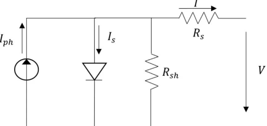
The detailed model with single diode has five parameters, further considering a shunt resistance [4, 35], as compared to the simple single diode model. This resistance accounts for “the losses due to the leakage currents across the junction and within the cell due to crystal imperfections and impurities” [4]. Figure 2.2.2 presents the equivalent circuit of this model.

Figure 2.1.2 – Equivalent circuit of single diode model considering both the shunt and series

resistances.

The current of the single diode detailed model, 𝐼, is determined by Eq. (4):

𝐼 = 𝐼𝑝ℎ− 𝐼𝑠(𝑒 𝑉+𝐼𝑅𝑠

𝑉𝑡 − 1) −𝑉 + 𝐼𝑅𝑠

𝑅_𝑠ℎ (4)

and where,

𝑅_𝑠ℎ - Module Shunt resistance [Ω].

Usually, the shunt resistance is much higher than the load resistance and, by comparison, the series resistance is much lower, so less power is dissipated [7]

𝑅

𝑅

𝑉

𝐼

𝐼

16

2.1.3 Double diode model

The double diode model includes another diode in parallel in the equivalent circuit. This diode accounts for “the losses due to the carrier recombination in the space charge region of the junction, and those due to surface recombination”. The first diode is responsible for the component of diffusion current. In this case, an additional parameter is included through the reverse saturation current of the second diode, while the ideality factors are known for both diodes [4]. The equivalent circuit of this model is shown in Figure 2.2.3.

Figure 2.1.3 – Equivalent circuit of the double diode model.

The current of the double diode model, 𝐼, is determined by equation (5):

𝐼 = 𝐼_𝑝ℎ− 𝐼_𝑠1(𝑒𝑉+𝐼𝑅𝑉𝑡 𝑠− 1) − 𝐼_𝑠2(𝑒

𝑉+𝐼𝑅𝑠

2𝑉𝑡 − 1) −𝑉 + 𝐼𝑅𝑠

𝑅_𝑠ℎ (5)

and where,

𝐼_𝑠1 – Dark saturation current of the first diode modelling the diffusion current component [A]; 𝐼_𝑠2 – Dark saturation current of the second diode modelling the recombination in the space charge region [A].

2.1.4 Considerations on photovoltaic cell models

In the single diode model, the diode ideality factor accounts for the effect of recombination in the space-charge region. This model is less accurate than the double diode model at lower values of incident irradiance, and can result in negative values of the series resistance. When the irradiance values are higher, this model predicts those values with significant differences, not offering constant results. The double diode model includes the space-charge recombination effect, because “a separate current component with its own exponential

𝑅

𝑅

𝑉

𝐼

𝐼

𝐼

𝐼

17

voltage dependence” is modelled. This model is described as being a more accurate description of the solar cell performance than that of the single-diode [16]. The single diode detailed model is sometimes referred to as the five-parameters model [4].

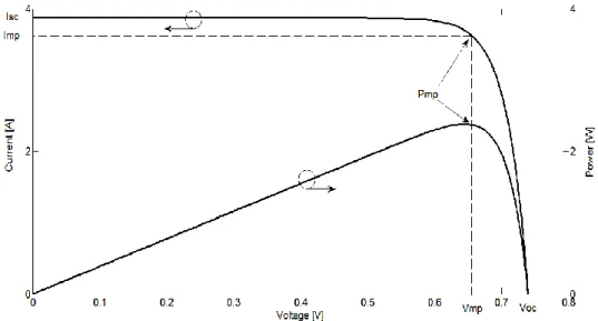
The characteristic curve of a solar cell is the relation between current and voltage, for a certain given irradiance, 𝐺𝑡, and a cell temperature, 𝑇𝑐. The convention imposes as positive the

current produced by the cell when receives solar radiation, and as positive the voltage that is, in that way, applied to the terminal of the cell. If the cell is short-circuited, the current has its maximum value, and the correspondent voltage is zero. If the circuit is open, the voltage value has its maximum, and the correspondent current is zero. These two points are extremely important to recognise the I-V curve, and between them the power output is higher than zero [7]. Figure 2.2.4 presents the I-V and P-V curves between those points.

Figure 2.1.4 – I-V and P-V curves representation, with the relevant current and voltage values.

Usually, these models fit experimental I-V characteristics accurately, and are often useful to obtain the model parameters. The parameters could be used to design the cell or module, and could be determined to optimize its performance. Also, “the model parameters can be a useful tool for monitoring cell manufacturing processes if the parameter values can be determined simply and rapidly” [16]. Due to the fact of being a first approach, we choose to work with the single diode model, considering the five parameters.

18

2.2 Determination of the characteristic current-voltage curve

Equation (4), in contrast to what happens with linear and quadratic algebraic functions, is a non-linear and transcendent equation that does not present an explicit analytical formula for its resolution, existing the need of finding numerical methods to solve it. A root finding algorithm is a numerical method or algorithm that allows finding a value 𝑥 such that 𝑓(𝑥) = 0, for a given function 𝑓. The 𝑥 is called the root of that function [18]. In order to obtain the solution of the equation that describes the net current of the solar cell, one must take advantage of methods that deal with iterative processes. Those methods start by knowing approximated values of the root we want to find [18]. Examples of those methods are Bisection method, False Position method, Secant method, Newton method, 𝑀𝑢̈𝑙𝑙𝑒𝑟 method [18].

The iterative process generates a succession of values, 𝑧_𝑘, with associated errors, as

𝑒𝑘 = 𝑥 − 𝑧𝑘 (6)

and because the iterative process should be a convergent process, it should be verified that: lim

𝑘→∞𝑧𝑘 = 𝑥 (7)

The same is to say that

lim

𝑘→∞𝑒𝑘 = 0 (8)

In [18] it is demonstrated how that error evolves with the number of iterations, and concluded that, in principle, if convergence rate is high, the number of iterations is small, depending on the required precision or tolerance. Although, this conclusion is not absolute and could lead to mistakes, because computational effort required must be considered. The main difference between local convergence methods and global convergence methods is that the firsts need to have initial values (starting values for the algorithms) as closer as possible of the solution we want to find, and the seconds do not [18].

19

2.2.1 Bisection method (Binary-Search or Bolzano)

Being 𝑓 a continuous function in the finite interval 𝑆 = [𝑎, 𝑏], and such that 𝑓 (𝑎) and 𝑓 (𝑏) have different signs, then function 𝑓 have at least one zero (root) in that interval. Bisection method consists in constructing subintervals 𝑆𝑘 = [𝑎𝑘, 𝑏𝑘] ⊂ 𝑆 = [𝑎, 𝑏] by

successive divisions in halfs, for which also verifies that 𝑓(𝑎𝑘) and 𝑓(𝑏𝑘) have opposite signs

[18]. In this way, a function root is being bound to successively smaller intervals. A schematic illustration was made for this numerical algorithm, presented in Figure 2.3.1.

Figure 2.2.1 - Bisection method schematic illustration. Adapted from [18].

The algorithm flowchart of the Bisection method appliance is shown in Figure 2.3.2.

Figure 2.2.2 – Bisection method algorithm flowchart.

𝑦 𝑦 = 𝑓(𝑥)

𝑎_𝑘 𝑥 _𝑎 𝑘+1_𝑘+1

𝑏_𝑘 𝑏𝑘+1

20

2.2.2 Secant method

Secant method consists of guessing two initial values, (𝑥_𝑘−1, 𝑓(𝑥_𝑘−1)) and (𝑥𝑘, 𝑓(𝑥𝑘)), and

obtain a next one, 𝑥𝑘+1, as the intersection of the secant defined by those points with

the 𝑥𝑥 axis, as can be seen in the schematic illustration of this method presented in Figure 2.3.3.

Figure 2.2.3 - Secant method schematic illustration. Adapted from [18].

The expression that allows obtaining the 𝑥_𝑘+1 value is

𝑥_𝑘+1 =𝑓(𝑥𝑘)𝑥𝑘−1− 𝑓(𝑥𝑘−1), 𝑥𝑘

𝑓(𝑥𝑘) − 𝑓(𝑥𝑘−1) (10)

The algorithm flowchart of the Secant method appliance is presented in Figure 2.3.4.

Figure 2.2.4 - Secant method algorithm flowchart.

𝑦 = 𝑓(𝑥) 𝑥𝑘−1 𝑥 𝑦 𝑓(𝑥𝑘−1) 𝑥𝑘 𝑥𝑘+1 𝑓(𝑥𝑘)

21

2.2.3 Newton-Raphson method

In the Newton-Raphson method, or simply Newton method, the curve is approximated with its tangent, as the schematic illustration of the method shows in Figure 2.3.5. The tangent intercepts the 𝑥𝑥 axis and this point is used as the new value of the approximation to the 𝑓 root. The equation of the tangent to the function 𝑓 at the point 𝑥_𝑘 is:

𝑦 = 𝑓(𝑥𝑘) + 𝑓′(𝑥𝑘)(𝑥 − 𝑥𝑘) (11)

The intersection with the 𝑥𝑥 axis occurs in the value obtained from the following expression

𝑥𝑘+1= 𝑥𝑘−

𝑓(𝑥𝑘)

𝑓′(𝑥_𝑘) (12)

In this case, it is required to guess an initial value of 𝑥0, which generate a succession {𝑥𝑘}

that will converge to the root of the function 𝑓. It is also required to compute its derivative, 𝑓′.

Figure 2.2.5 - Newton-Raphson method schematic illustration. Adapted from [18].

The algorithm flowchart of the Newton-Raphson method appliance is presented in Figure 2.3.6. 𝑦 = 𝑓(𝑥) 𝑥𝑘 𝑥 𝑦 𝑥𝑘+1 𝑓(𝑥𝑘)

22

Figure 2.2.6 - Newton-Raphson algorithm flowchart.

2.3 Application results

Bisection, Newton-Raphson and Secant methods were studied and applied in order to conclude which one of those algorithms is the best suited to make the description of the current-voltage curve. To apply the methods, ideal five parameters were used, described in Table 2.4.1, at a cells temperature of 25.00℃, which corresponds to 298.15𝐾.

Table 2.3.1 - Parameters ideal values.

Parameter 𝐼𝑝ℎ [𝐴] 𝐼𝑠 [𝐴] 𝑛 𝑅𝑠ℎ [Ω] 𝑅𝑠 [Ω]

Value 3.80 1.00 × 10−10 1.20 1.00 × 105 1.00 × 10−5

2.3.1 Bisection method

Bisection method was used to solve the current equation in the interval: [0.00-20.00] A, with an absolute error of 10−8_{, and in a voltage interval [0.00-0.76] V. The error is the difference}

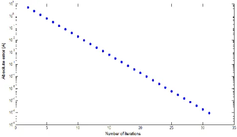
between successive values of current between the iterations. The method takes several iterations until convergence is reached (namely thirty-one iterations, in this case), and the variation of the estimated error is presented in Figure 2.4.1, with all those iterations represented.

23

Figure 2.3.1 - Error of Bisection method cycle, as a function of the number of iterations.

The stopping criterion is the absolute error of the calculated current, which is updated in each iteration step. In those conditions, thirty-one iterations were required. The result of this iteration procedure is the current in the circuit, for each given value of voltage.

2.3.1.1 Considerations

A rigorous convergence and error analysis of Bisection method is made in [18]. The Bisection method guarantee that convergence is always obtained in the defined interval for continuous functions, concluding that it is a global method. However, its convergence rate can be slow. This is the main reason why, generally, this method is used in a first phase of the works [18].

2.3.2 Secant method

To initiate the iteration procedure of the Secant method two initial values were required. Starting values of 𝑥_𝑘−1 of 3.70 A, and 𝑥_𝑘 of 3.80 A were used in this case. The absolute error of the current was 10−8_{, same as above. To verify if the method has the same response for all}

the voltage values used, the method was analysed independently for three distinct values: for the initial value of voltage range (0.00 V), a value in the middle of the voltage range (0.37 V), and a value near the end of the voltage range (0.73 V). The results are shown in the Table 2.4.2.

24

Table 2.3.2 – Secant application results.

Voltage [V] Iteration number Current [A]

0.00 1 3.886924999611179 2 3.886924999611179 0.37 1 3.886901373154788 2 3.886901373154771 0.73 1 1.037954603564634 2 1.037953465021237 3 1.037953465020754

One can see in Table 2.4.2 that the function converges in two iterations in the beginning and middle of the interval of the voltage, and in the end of that interval the function converges in three iterations. In this way, one can conclude that the more far the solution is from the initial guessed values, a higher number of iterations are required.

2.3.2.1 Considerations

In this method, it is not required that the values of the function in subintervals extremes have different signs, which could mean that in some cases convergence is not absolute. The theoretical demonstration of Secant method convergence and error analysis is made in [18]. This method must be evaluated before use, in order to have the guarantee that the convergence is obtained with the function. Since Eq. (4) do not presented convergence problems, it was concluded that the method was well suited to use.

2.3.3 Newton Raphson method

Newton-Raphson method was applied to Equation (4), for the same conditions explained above. To start the iteration procedure of this method, an initial value of current, 𝑥𝑘, of 3.80

A was used. The function was applied to the same values of voltage presented before in 2.4.2, in the Secant method. The results of Newton-Raphson method are shown in Table 2.4.3.

25

Table 2.3.3 - Newton-Raphson application results.

Voltage [V] Iteration number Current [A]

0.00 1 3.886924999611179 2 3.886924999611179 0.37 1 3.886901373154779 2 3.886901373154771 0.73 1 1.037954646347110 2 1.037953465020761 3 1.037953465020754

It can be seen that convergence is obtained in two iterations for the values in the lower end and middle of the voltage range, and in the upper end of that range three iterations are required. Newton-Raphson method convergence is fast with an initial value close to the solution.

2.3.3.1 Considerations

The Newton-Raphson method, as in the case of the Secant method, may present convergence problems, and so a convergence and error analysis is explained in [18]. It is important to note that this method requires evaluating the derivative of the function, and so if the function is a very complex analytical expression, its derivative and computational programming become difficult, and so the choice of this method must be weighted. Because the convergence is quadratic, the Newton-Raphson method is one of the most used methods to non-linear equations [18]. In this case, using the Newton method with Eq. (4) did not showed any problem of convergence, and it is concluded that it is suitable method in this case.

2.4 Coupling Bisection and Newton-Raphson methods

Bisection method gives the guarantee of convergence; however, its slower convergence rate is a drawback. On the other hand, the Newton-Raphson method is the fastest one, due to its higher convergence rate (quadratic), which means that the accuracy is doubled in each one of the iterations [18]. Additionally, for some complex functions, the convergence of the method it is not guaranteed, which however it is not the case of Equation (4). Secant method is a fast method because it is a Newton-Raphson derivation, and it was interesting to analyse how to

26

ensure that derivative of the function offer no problem. Nevertheless, if initial value is not close to the root, there is no guarantee that the solution is reached, the same happening in the case of the Newton-Raphson method.

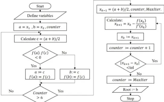
Taking into consideration the facts presented before, an idea to save a lot of computer processing, time and costs arise. The solution is to combine two of the methods presented before, namely the Bisection and Newton methods. The Bisection method should initiate the iteration procedure, and so one can assure that the method will converge. Because the function under study do not present problems in computing its derivative, Newton-Raphson method was chosen. The flowchart that describes the algorithm of the coupling of these two methods is shown in Figure 2.5.1.

Figure 2.4.1 – Flowchart for coupling Bisection and Newton Raphson methods.

2.4.1 Application results

For the coupled method, the same initial conditions as used before in Bisection method were also used. After a few iterations with Bisection method, the output value of current in that present iteration is taken and becomes the initial value of the Newton-Raphson method. In other words, from that iteration Bisection offers a good approximation of the solution to Newton-Raphson method, were this one starts and finish the iteration procedure.

Table 2.5.1 shows the result of the iterative process, which starts with Bisection method and after the 6𝑡ℎ _{iteration the algorithm changes to Newton-Raphson method that converges to}

27

Table 2.4.1 – Results with coupled methods.

Voltage [V] 0.00 0.37 0.73

Method Number of

iterations Current [A]

Bisection 1 5.00000000000000 5.00000000000000 5.00000000000000 2 2.50000000000000 2.50000000000000 2.50000000000000 3 3.75000000000000 3.75000000000000 1.25000000000000 4 4.37500000000000 4.37500000000000 0.62500000000000 5 4.06250000000000 4.06250000000000 0.93750000000000 6 3.90625000000000 3.90625000000000 1.09375000000000 Newton-Raphson 1 3.88692499961118 3.88690137315478 1.03795346509791 2 3.88692499961118 3.88690137315477 1.03795346502076

This combined method allows a significant improvement of both methods in the way that convergence rate of Bisection method is not so slow and we have the insurance that Newton-Raphson method will converge to the solution because the initial guesses of the method are not so far from the solution. We can see that the function that describes the net current converges in a total of eight iterations starting from the same initial values as the pure Bisection method, which needed thirty-one iterations to converge. The photovoltaic cell output with this combined Bisection and Newton-Raphson methods is shown in Figure 2.5.2. With those conditions, the maximum power output is 2.43 W.

28

3 Chapter 3 - Parameters determination using the Nelder and Mead algorithm

The work presented in this chapter was developed aiming to describe and validate the Nelder and Mead algorithm applied to the determination of the five parameters of a photovoltaic module. The analysis is based in the values of the I-V characteristic curve, which are simulated based in the available data of a module. The response of the algorithm will be evaluated in three main paths, namely, the initial simplex maximum deviation, the imposed noise value of the current and the tolerance.

3.1 Determination of the parameters of a module

Previous section simulations were made using five ideal parameters. In this section, the five parameters which characterize the cell and module will be determined.

Parameters identification could be divided into three main categories, the analytical methods, which were investigated by many authors, as for example [16], the numerical methods, such as Newton-Raphson or Pattern Search, and the hybrid methods, such as cuckoo search hybridized with Nelder-Mead simplex (CS-NMS) [36]. These three main classes are summarized in Figure 3.1.1.

Parameters determination

using the Nelder and

Mead algorithm

Chapter 3

-

Paramete

rs

determin

ation

using the

Nelder