Impact analysis of travel time uncertainty on AGV catch-up conflict and the associated dynamic adjustment

(1)

Research Article

Impact Analysis of Travel Time Uncertainty on AGV Catch-Up

Conflict and the Associated Dynamic Adjustment

Jun-jun Li

,

1

Bo-wei Xu

,

2

Octavian Postolache

,

3

Yong-sheng Yang

,

2

and Hua-feng Wu

1

1_{Merchant Marine College, Shanghai Maritime University, Shanghai 201306, China}

2_{Institute of Logistics Science & Engineering, Shanghai Maritime University, Shanghai 201306, China} 3_{Instituto de Telecomunicacoes, ISCTE-IUL, Av. Das Forcas Armadas, 1049-001 Lisbon, Portugal}

Correspondence should be addressed to Bo-wei Xu; [email protected]

Received 3 September 2017; Revised 31 December 2017; Accepted 11 February 2018; Published 19 April 2018 Academic Editor: Francisco Chicano

Copyright © 2018 Jun-jun Li et al. This is an open access article distributed under the Creative Commons Attribution License, which permits unrestricted use, distribution, and reproduction in any medium, provided the original work is properly cited. In automated logistics systems, travel time uncertainty can severely affect automated guided vehicle (AGV) conflict and path planning. Insight is required into how travel time uncertainty affects catch-up conflict, the main AGV conflict in one-way road networks. Under normal circumstances, the probability formula for catch-up conflict is deduced based on an analysis of AGV catch-up conflict. The vertex, monotonicity, and symmetry of catch-up conflict probabilities are developed, for symmetrical AGV travel time distribution densities. A dynamic adjustment method based on conflict probability for AGVs is designed. The probability features of catch-up conflicts and the performance of the associated dynamic adjustment are simulated and validated for AGVs at an automated container terminal. The simulation results show that the impact analysis of travel time uncertainty on AGV catch-up conflict is correct, and the dynamic adjustment is effective.

1. Introduction

Automated guided vehicles (AGVs) participate in unmanned transport systems for material handling [1]. In automated logistics systems, such as automated container terminals and automated warehouses, conflicts may arise when several AGVs run along a narrow lane or pass crossing roads [2]. AGV conflict (which can significantly affect actual AGV speeds, expected travel time, and automated logistic system throughput) has been a key issue in AGV path planning [3]. Many studies have focused on conflict avoidance strategies when studying AGV path planning [1, 4, 5]. Smolic-Rocak et al. used time window insertion in vector form and performed window overlapping tests to dynamically solve the shortest path problem for the supervisory control of AGVs traveling within the layout of a given warehouse [4]. Saidi-Mehrabad et al. considered a conflict-free routing problem (CFRP) for AGVs, as well as a basic job shop scheduling problem (JSSP) to minimize total completion time (make-span). They proposed a two-stage ant colony algorithm

(ACA) for this problem, especially for large-size problems [1]. Hidalgo-Paniagua et al. proposed a new multiobjective evolutionary approach based on a variable neighborhood search to produce good paths with shorter lengths, improved safety, and smoother mobile robot movements [5]. However, AGV transportation systems are subject to a high degree of uncertainty [6]. The above references simplified AGV conflict avoidance strategies for deterministic conditions, which might lead to suboptimal or even infeasible solutions. In the real world, AGV conflict on road networks is highly affected by AGV travel times, which are very uncertain because of roadway capacity variations and traffic demand fluctuations [7, 8]. Therefore, the on-time arrival probability of AGVs in automated logistics systems cannot be ensured, especially for a large number of AGVs operating in a limited area. An interesting queuing approach is used to model rout-ing problems with time-dependent travel time [9]. Strategies have been proposed to avoid stochastic travel time influence against unpredictable and random conflicts [10, 11]. Shao et al. used a two-stage traffic control strategy to resolve conflicts

Volume 2018, Article ID 4037695, 11 pages https://doi.org/10.1155/2018/4037695

(2)

and deadlock problems in AGV systems. Specifically, a traffic controller is employed to operate each moving AGV online

after utilizing an A∗algorithm to offline construct an optimal

path set for AGVs [10]. Zhang et al. formulated on-time ship-ment delivery problems as stochastic vehicle routing prob-lems with soft time windows under travel and service time uncertainties and proposed a new stochastic programming model for finding a good trade-off between the total cost borne by carriers and customer service levels [11]. However, measures such as scheduling methods and control strategies, which can temporarily prevent conflicts, may reduce the effi-ciency of AGV systems. Exclusive dependence on these mea-sures easily leads to queuing and congestion in heavy traffic. Therefore, reasonably preanalyzing AGV conflicts under random circumstances can facilitate shorter travel times and higher AGV utilization rates. However, there is not a way to compute the probability of AGV conflicts under uncertainty. Dynamic adjustment is a key measure to deal with con-flicts in the operations management of AGV systems. Lee et

al. employed a𝑘-shortest path search algorithm to construct

a path set and performed online motion planning operation in real time [12]. Li et al. proposed a set of real-time imple-mentable traffic rules to ensure the completion of all jobs with the absence of vehicle deadlocks and collisions [13]. Hoo-Lim et al. proposed a genetic algorithm to continuously optimize and adjust the traffic flow of AGVs for keeping up with the dynamically changing operational condition [14]. Different adjust strategies may result in different running state and dif-ferent productivity. It is better to analyze conflict probabilities and perform associated dynamical adjustment, rather than employ traditional adjustment as passive response measures to avoid conflicts among AGVs. Furthermore, many methods mentioned in the literature did not consider conflict proba-bilities in advance of dynamic adjustment, which might bring high frequency of control action, high operational cost, low efficiency, and service ability of automated logistics systems.

After studying the current literature, it is clear that the analysis of AGV conflicts under uncertainty has received less attention from the research community. In this work, catch-up conflict (the main type of AGV conflict in a one-way road network) probability and the associated dynamic adjustment are studied. Compared with the existing literature, the main contributions of this work are elucidated as follows. First, to meet the needs of operation management, AGVs’ travel times are set to random values and the AGV catch-up conflict problem in one-way and single lane road networks is described. Second, the catch-up conflict probability features are analyzed in detail in a situation where the probability density function for the times of AGVs passing through each node is symmetrical. Finally, the dynamic adjustment based on the conflict probability for AGVs is presented in order to reduce catch-up conflicts among AGVs.

2. AGV Catch-Up Conflict Probability and

Uncertain Travel Time

2.1. AGV Catch-Up Conflict Probability. A one-way and single

lane road network for an automated logistic system is denoted

by a graph with𝑁 nodes (𝐴₁, 𝐴₂, . . . , 𝐴_𝑁) and 𝐵 links. 𝐴_𝑘

and𝐴_𝑙are the𝑘th and 𝑙th nodes, respectively, and they are

consecutive. There are 𝑃 AGVs (AGV₁, AGV₂, . . . , AGV_𝑃).

The start node and end node of the𝑝th AGV (denoted as

AGV_𝑝) are𝑆𝑝and𝐸𝑝, respectively.

Assume that AGV_𝑝passes through node𝐴_𝑘at time𝑡_𝑝,𝑘.

The probability density function and cumulative distribution

function for time𝑡_𝑝,𝑘are𝜑_𝑝,𝑘(𝑡) and 𝐹_𝑝,𝑘(𝑡), respectively. ∀𝑡 ∈

(−∞, +∞), 𝜑𝑝,𝑘(𝑡) < +∞. Once 𝑡𝑝,𝑘 ≤ 𝑡𝑞,𝑘and𝑡𝑝,𝑙 ≥ 𝑡𝑞,𝑙, or

𝑡_𝑝,𝑘 ≥ 𝑡_𝑞,𝑘 and𝑡_𝑝,𝑙 ≤ 𝑡_𝑞,𝑙, catch-up conflicts occur between

AGV_𝑝 and AGV_𝑞 (the 𝑞th AGV). A situation where two

AGVs repeatedly catch up with one another is not considered here.

Assuming that the movements of AGVs are mutually

independent, the events 𝑡_𝑝,𝑘 ≤ 𝑡_𝑞,𝑘 and 𝑡_𝑝,𝑙 ≥ 𝑡_𝑞,𝑙 are

independent of one another. Additionally,𝑡_𝑝,𝑘 ≥ 𝑡_𝑞,𝑘 and

𝑡_𝑝,𝑙 ≤ 𝑡_𝑞,𝑙are independent events. The probability of AGV

catch-up conflict event𝜍 is 𝑃(𝜍). It can be shown that

𝑃 (𝜍) = 𝑃 (𝑡𝑝,𝑘≤ 𝑡𝑞,𝑘) ⋅ 𝑃 (𝑡𝑝,𝑙≥ 𝑡𝑞,𝑙) + 𝑃 (𝑡𝑝,𝑘≥ 𝑡𝑞,𝑘) ⋅ 𝑃 (𝑡_𝑝,𝑙≤ 𝑡_𝑞,𝑙) , (1) where𝑃(𝑡_𝑝,𝑘≤ 𝑡_𝑞,𝑘) is shown in 𝑃 (𝑡_𝑝,𝑘≤ 𝑡_𝑞,𝑘) = ∫+∞ −∞ 𝜑𝑞,𝑘(𝜏) ∫ 𝜏 −∞𝜑𝑝,𝑘(𝑡) 𝑑𝑡 𝑑𝜏 = ∫+∞ −∞ 𝜑𝑞,𝑘(𝜏) 𝐹𝑝,𝑘(𝜏) 𝑑𝜏 (2) ∵ ∀𝑡 ∈ (−∞, +∞), 𝜑_𝑝,𝑘(𝑡) < +∞, ∴ ∫_𝜏𝜏𝜑_𝑝,𝑘(𝑡)𝑑𝑡 = 0. ∴ 𝑃(𝑡_𝑝,𝑘= 𝑡_𝑞,𝑘) = ∫_−∞+∞𝜑_𝑞,𝑘(𝜏) ∫_𝜏𝜏𝜑_𝑝,𝑘(𝑡)𝑑𝑡 𝑑𝜏 = 0.

In this case,𝑃(𝜍) is shown in

𝑃 (𝜍) = 𝑃 (𝑡𝑝,𝑘≤ 𝑡𝑞,𝑘) ⋅ [1 − 𝑃 (𝑡𝑝,𝑙≤ 𝑡𝑞,𝑙)]

+ [1 − 𝑃 (𝑡_𝑝,𝑘≤ 𝑡_𝑞,𝑘)] ⋅ 𝑃 (𝑡_𝑝,𝑙≤ 𝑡_𝑞,𝑙)

= 𝑃 (𝑡_𝑝,𝑘≤ 𝑡_𝑞,𝑘) + 𝑃 (𝑡_𝑝,𝑙≤ 𝑡_𝑞,𝑙) − 2𝑃 (𝑡_𝑝,𝑘≤ 𝑡_𝑞,𝑘)

⋅ 𝑃 (𝑡_𝑝,𝑙≤ 𝑡_𝑞,𝑙) .

(3)

Let the times at which AGV_𝑞passes through nodes𝐴_𝑘

and𝐴_𝑙be𝑡_𝑞,𝑘+𝑥 and 𝑡_𝑞,𝑙+𝑥, respectively, where 𝑥 indicates the

change in departure time for AGV_𝑞. Meanwhile, let𝑔₁(𝑥) =

𝑃(𝑡_𝑝,𝑘 ≤ 𝑡_𝑞,𝑘+ 𝑥 ), 𝑔₂(𝑥) = 𝑃(𝑡_𝑝,𝑙 ≤ 𝑡_𝑞,𝑙+ 𝑥 ) and 𝑧(𝑥) = 𝑃(𝜍).

From (3), it is determined that

𝑧 (𝑥) = 𝑔1(𝑥) + 𝑔2(𝑥) − 2𝑔1(𝑥) ⋅ 𝑔2(𝑥) . (4)

2.2. Uncertain Travel Time

2.2.1. Travel Time Is Random. In an automated logistic

sys-tem, some AGVs may have the same design speed. If an AGV

travels exactly at the design speedV₀, then its arrival time

at a node is𝑡 = 𝑡₀. In practice, because of uncertainty (e.g.,

(3)

the actual arrival time is a random variable. Assuming that the various uncertainties are arbitrary, the probability density function of the random variable would be symmetrical about

𝑡 = 𝑡₀.

Two probability distribution functions (uniform distribu-tion [8, 15] and normal distribudistribu-tion [15, 16]) widely used in engineering are specified in (5) and (6), respectively.

𝜑 (𝑡) ={_{ { 0.5 𝛿 , 𝑡 ∈ (𝑡0− 𝛿, 𝑡0+ 𝛿) 0, else, (5) 𝜑 (𝑡) = 1 √2𝜋𝜎𝑒−(𝑡−𝑡0) 2_/2𝜎2 , (6) where𝛿 > 0, 𝜎 > 0.

2.2.2. Travel Speed Is Random. When the speeds of AGVs

change randomly, the times at which the AGVs pass through

nodes become random. Here,V_𝑝 denotes the actual speed

of AGV_𝑝. Similar to (5) and (6), the uniform and normal

distributions ofV_𝑝are given in (7) and (8), respectively.

𝜙 (V) ={_{ { 0.5 𝛿󸀠, V ∈ (V0− 𝛿󸀠, V0+ 𝛿󸀠) 0, else (7) 𝜙 (V) = 1 √2𝜋𝜎󸀠𝑒 −(V−V0)2/2𝜎󸀠2_, ₍₈₎

where𝛿󸀠> 0, 𝜎󸀠> 0. If the departure time of AGV_𝑝is𝑥, then

the time at which it passes through node𝑘 is 𝑡_𝑝,𝑘= 𝑥 +𝐿_𝑝,𝑘/V_𝑝,

where𝐿_𝑝,𝑘is the distance traveled by AGV_𝑝from node𝑆𝑝to

node𝑘. If the probability density function of V_𝑝is𝜙_𝑝(V), then

the probability density function of𝑡_𝑝,𝑘is

𝜑_𝑝,𝑘(𝑡) = 𝐿𝑝,𝑘

(𝑡 − 𝑥)2𝜙𝑝(

𝐿𝑝,𝑘

𝑡 − 𝑥) . (9)

In Section 3, the impact of travel time uncertainty on catch-up conflict described in Section 2.1 is analyzed; subsequently, catch-up conflicts caused by uncertain travel time described in Section 2.2 are simulated in Section 5.

3. Impact of Travel Time Uncertainty on

Catch-Up Conflict

The catch-up conflict between two AGVs is the basis for catch-up conflicts among multiple AGVs. Catch-up conflict

probabilities between AGV_𝑝and AGV_𝑞are analyzed here.

First, on the basis of distribution characteristics of

𝑃(𝑡_𝑝,𝑘 ≤ 𝑡_𝑞,𝑘 + 𝑥 ) and 𝑃(𝑡_𝑝,𝑙 ≤ 𝑡_𝑞,𝑙 + 𝑥 ), the symmetry

and monotonicity of 𝑃(𝜍) are analyzed by Theorem 1 and

Inference 2, respectively. Second, according to the

symme-tries of𝜑_𝑝,𝑘(𝑡) and 𝜑_𝑞,𝑘(𝑡), the symmetry of 𝑃(𝑡_𝑝,𝑘 ≤ 𝑡_𝑞,𝑘+

𝑥) is analyzed using Theorem 3. Finally, the distribution

characteristics of𝑃(𝜍) are comprehensively analyzed using

Inference 4.

Theorem 1. If 𝑃(𝑡_𝑝,𝑘 ≤ 𝑡_𝑞,𝑘 + 𝑥 ) and 𝑃(𝑡_𝑝,𝑙 ≤ 𝑡_𝑞,𝑙+ 𝑥 ) are

symmetric about point(𝑥₀, 0.5), then 𝑃(𝜍) is symmetric about

𝑥 = 𝑥₀and𝑧(𝑥₀) = 0.5.

Inference 2. If both 𝑃(𝑡_𝑝,𝑘 ≤ 𝑡_𝑞,𝑘) and 𝑃(𝑡_𝑝,𝑙 ≤ 𝑡_𝑞,𝑙) are

symmetric about point(𝑥₀, 0.5), and both 𝑔₁(𝑥) and 𝑔₂(𝑥)

monotonically increase (or monotonically decrease), then

𝑃(𝜍) is an increasing function when 𝑥 ≤ 𝑥₀, or vice versa.

Theorem 3. If 𝜑_𝑝,𝑘(𝑡) and 𝜑_𝑞,𝑘(𝑡) are symmetric about 𝑡 = 𝑡₁

and𝑡 = 𝑡₂, respectively, then𝑃(𝑡_𝑝,𝑘 ≤ 𝑡_𝑞,𝑘+ 𝑥 ) is symmetric

about point(𝑡₁− 𝑡₂, 0.5).

Inference 4. If the following conditions are met in AGV_𝑝and

AGV_𝑞:

(1) the times at which AGV_𝑝 and AGV_𝑞 pass through

node𝐴_𝑘are𝑡_𝑝,𝑘and𝑡_𝑞,𝑘+ 𝑥, respectively. The times at which

AGV_𝑝and AGV_𝑞pass through node𝐴_𝑙are𝑡_𝑝,𝑙and𝑡_𝑞,𝑙+ 𝑥,

respectively.

(2) 𝜑_𝑝,𝑘(𝑡), 𝜑_𝑞,𝑘(𝑡), 𝜑_𝑝,𝑙(𝑡), and 𝜑_𝑞,𝑙(𝑡) are the interval

distributions 𝜑_𝑝,𝑘(𝑡) > 0, 𝑡 ∈ (𝑐_𝑝,𝑘, 𝑑_𝑝,𝑘) , 𝜑_𝑝,𝑘(𝑡) = 0, 𝑡 ∉ (𝑐𝑝,𝑘, 𝑑𝑝,𝑘) , 𝜑𝑞,𝑘(𝑡) > 0, 𝑡 ∈ (𝑐𝑞,𝑘, 𝑑𝑞,𝑘) , 𝜑_𝑞,𝑘(𝑡) = 0, 𝑡 ∉ (𝑐_𝑞,𝑘, 𝑑_𝑞,𝑘) , 𝜑_𝑝,𝑙(𝑡) > 0, 𝑡 ∈ (𝑐_𝑝,𝑙, 𝑑_𝑝,𝑙) , 𝜑𝑝,𝑙(𝑡) = 0, 𝑡 ∉ (𝑐𝑝,𝑙, 𝑑𝑝,𝑙) , 𝜑_𝑞,𝑙(𝑡) > 0, 𝑡 ∈ (𝑐_𝑞,𝑙, 𝑑_𝑞,𝑙) , 𝜑_𝑞,𝑙(𝑡) = 0, 𝑡 ∉ (𝑐_𝑞,𝑙, 𝑑_𝑞,𝑙) , (10)

respectively.𝑐_𝑝,𝑘,𝑑_𝑝,𝑘,𝑐_𝑞,𝑘,𝑑_𝑞,𝑘,𝑐_𝑝,𝑙,𝑑_𝑞,𝑙,𝑐_𝑞,𝑙, and𝑑_𝑞,𝑙are all real

numbers.𝑐_𝑝,𝑘< 𝑑_𝑝,𝑘,𝑐_𝑞,𝑘< 𝑑_𝑞,𝑘,𝑐_𝑝,𝑙< 𝑑_𝑞,𝑙, and𝑐_𝑞,𝑙< 𝑑_𝑞,𝑙.

(3)𝜑_𝑝,𝑘(𝑡), 𝜑_𝑞,𝑘(𝑡), 𝜑_𝑝,𝑙(𝑡), and 𝜑_𝑞,𝑙(𝑡) are symmetric about

𝑡 = 𝑡₁, 𝑡₂, 𝑡₃and𝑡₄, respectively, where𝑡₁− 𝑡₂= 𝑡₃− 𝑡₄.

Thence,𝑃(𝜍) is symmetric about 𝑥₀ = 𝑡₁ − 𝑡₂, and𝑃(𝜍)

conforms to Formula (11), where𝑆_𝑘= [𝑐_𝑝,𝑘− 𝑑_𝑞,𝑘, 𝑑_𝑝,𝑘− 𝑐_𝑞,𝑘],

𝑆_𝑙= [𝑐_𝑝,𝑙− 𝑑_𝑞,𝑙, 𝑑_𝑝,𝑙− 𝑐_𝑞,𝑙], 𝑆_𝑘∪ 𝑆_𝑙= [𝑎, 𝑏]. 𝑃 (𝜍) = 𝑧 (𝑥) is { { { { { { { { { { { { { { { 0.5, 𝑥 = 𝑥0 monotonically increasing, 𝑥 ∈ [𝑎, 𝑥₀] monotonically decreasing, 𝑥 ∈ [𝑥₀, 𝑏] 0, 𝑥∈ (−∞, 𝑎] ∪ [𝑏, +∞) . (11)

Similarly, if some intervals of (𝑐_𝑝,𝑘, 𝑑_𝑝,𝑘), (𝑐_𝑞,𝑘, 𝑑_𝑞,𝑘),

(𝑐_𝑝,𝑙, 𝑑_𝑝,𝑙), and (𝑐_𝑞,𝑙, 𝑑_𝑞,𝑙) change to closed intervals, Inference

4 is true; if one of these intervals is adjusted to(−∞, +∞)

(such as𝑐_𝑝,𝑘, 𝑑_𝑝,𝑘→ −∞) Inference 4 remains true.

The above analysis can provide premise and basis for dynamic adjustment and help to reduce catch-up conflicts among AGVs.

(4)

4. Dynamic Adjustment Based on

Conflict Probability

Dynamic adjustment based on conflict probability may change the traditional passive response mode to taking the initiative in avoiding conflicts among AGVs. This could pro-vide substantial productivity improvement for AGV trans-portation systems.

If all catch-up conflict probabilities are considered, the difficulty and complexity of AGVs planning will increase and the process would involve more calculation. Hence, based on the catch-up conflict probability features revealed

in Inference 4, a catch-up conflict probability threshold𝑇_ccp

(0 < 𝑇_ccp< 0.5) is considered for improving the efficiency of

AGVs planning. If the catch-up conflict probability is larger

than𝑇_ccp, then the AGVs with low priority replan their paths;

else, the AGVs with low priority simply slow down or wait to avoid conflicts once the potential catch-up conflicts happen. When the AGVs with low priorities replan their paths, the

links with “𝑃(𝜍) > 𝑇ccp” in path preplanning are eliminated

from their optional links in the corresponding time windows.

Checking “𝑃(𝜍) > 𝑇ccp” and path replanning by the AGVs

with low priorities are executed until “𝑃(𝜍) > 𝑇_ccp” does not

exist. Then all catch-up conflict probabilities are lower than

𝑇_ccp. Low conflict probabilities would result in few conflicts,

which will greatly reduce the negative impact of conflicts on AGVs operation.

Details are as follows.

The dynamic adjustment flow of AGVs is given in Figure 1. First, the priorities of AGVs are set, and the

catch-up conflict probability threshold𝑇_ccpis given. The steps of

dynamic adjustment are listed below.

Step 1. After path preplanning based on Dijkstra’s algorithm

for each AGV, it can be known whether different AGVs will pass through the same nodes. If such nodes do not exist, the AGVs will move according to their path plan; else, turn to Step 2.

Step 2. Calculate the catch-up conflict probability 𝑃(𝜍). If

𝑃(𝜍) > 𝑇_ccp, the AGVs with low priorities replan their paths

based on Dijkstra’s algorithm with time window and recheck

whether the catch-up conflict probability exceeds𝑇_ccpuntil

the catch-up conflict probability is lower than𝑇_ccp; else, turn

to Step 3.

Step 3. AGVs travel according to their path planning. In the

process of AGVs traveling, the potential catch-up conflicts are detected by sensors on AGVs. If a catch-up conflict is predicted to occur, the AGVs with low priorities slow down or wait to avoid conflicts; else, AGVs move on.

In the dynamic adjustment based on conflict probability,

it is important to check “𝑃(𝜍) > 𝑇_ccp.” However, it is different

from detecting potential conflicts. On the one hand, “𝑃(𝜍) >

𝑇_ccp” is checked by calculation, while potential conflicts are

detected by sensors. On the other hand, checking “𝑃(𝜍) >

𝑇ccp” is just after AGVs path preplanning and before AGVs

starting to move, whereas, detecting potential conflicts is

Y Y Y N N N

Does catch-up conflict probability exceed the threshold?

AGVs with low priorities replan path Do different AGVs pass

through the same nodes?

Is a catch-up conflict predicted to occur?

AGVs with low priorities slow down or wait to avoid conflicts

AGVs move on AGVs path preplanning

AGVs move

Potential catch-up conflicts are detected by sensors on AGVs

Figure 1: Dynamic adjustment based on conflict probability.

ahead of the node that AGVs will reach and in the process of AGVs moving.

5. Simulations on Catch-Up Conflict

5.1. Simulation Settings. Automated container terminals are

typical automated logistics systems. Because of the notable uncertainty characteristics at automated container terminals, conflicts among AGVs are particularly common, resulting in new bottlenecks of loading and unloading operations. Therefore, it is extremely important to take AGVs at auto-mated container terminals as an example for analyzing catch-up conflict probabilities, using simulations to enhance the operational abilities of AGVs and improve the overall efficiency of automated container terminals. Figure 2 shows the road network of an automated container terminal. Roads in the network are one-way and single lanes. “QC” and “YC” indicate the quay crane and yard crane, respectively.

V₀is 5 m/s. The horizontal and vertical path lengths are 260

and 90 m, respectively. Nodes 1–63 are road network nodes.

(5)

1 2 3 5 6 8 9 14 15 17 18 26 28 29 31 32 30 30 30 30 20 30 10 10 10 60 D/m a 64 d 67 e 68 f 69 b 65 c 66 g 70 4 13 27 20 7 16 30 30 12 20 21 23 24 22 25 10 19 33 20 20 11 37 38 41 42 53 56 57 60 61 35 55 39 58 34 45 46 49 51 48 52 44 63 A B C 36 43 47 50 54 59 62 40 10 YC QC D: distance ！＇６p ！＇６q

Figure 2: Road network layout and AGVs’ paths at an automated container terminal.

following parameters are defined based on the statistics of an actual automated container terminal with annual throughput capacity of 5 million TEU.

The red and purple lines denote the travel paths of AGV_𝑝

and AGV_𝑞, respectively. Both AGV_𝑝and AGV_𝑞pass through

link (28, 29), which may cause catch-up conflict. It can be

calculated that𝑡₁ = 20 s,𝑡₃ = 26 s,𝑡₂= 4 s, and𝑡₄ = 10 s. If

the departure time of AGV_𝑝and AGV_𝑞is both 0 s, let𝑡_𝑝,28

and𝑡_𝑝,29denote the actual times at which AGV_𝑝reach nodes

28 and 29, respectively, and let𝑡_𝑞,28and𝑡_𝑞,29denote the actual

times at which AGVqreach nodes 28 and 29, respectively. The

departure time of AGV_𝑞 changes to𝑥 s; the actual times at

which AGV_𝑞reach nodes 28 and 29 are𝑡_𝑞,28+ 𝑥 and 𝑡_𝑞,29+ 𝑥,

respectively. Here,𝑃(𝜍) = 𝑧(𝑥) is simulated to verify the

impact analysis of travel time uncertainty on catch-up conflict in Section 3.

𝜑(𝑡) in (5) and (6) are employed in 𝜑_𝑝,28(𝑡), 𝜑_𝑞,28(𝑡),

𝜑_𝑝,29(𝑡), and 𝜑_𝑞,29(𝑡). For the convenience, 𝛿_𝑝and𝜎_𝑝denote

𝛿 and 𝜎 in 𝜑_𝑝,28(𝑡) and 𝜑_𝑝,29(𝑡), respectively, while 𝛿_𝑞and𝜎_𝑞

denote𝛿 and 𝜎 in 𝜑_𝑞,28(𝑡) and 𝜑_𝑞,29(𝑡), respectively.

Inference 4 in Section 3 is a summary of the conflict prob-ability characteristics. Therefore, only Inference 4 is verified in Section 5. Both “Conditions of Inference 4 are exactly met” and “Conditions of Inference 4 are approximately met” are simulated with MATLAB.

5.2. Conditions of Inference 4 Are Exactly Met

5.2.1. 𝜑(𝑡) Is Unrelated to Travel Distance. 𝛿 and 𝜎 in (5) and

(6) remain constant. Generally, the times at which an AGV passes through adjacent nodes obey the same type of prob-ability distribution. According to different combinations of uniform and normal distributions, there are three situations

Table 1: Distributions and parameters in𝜑(𝑡).

𝜑_𝑝,28(𝑡), 𝜑_𝑝,29(𝑡) 𝜑_𝑞,28(𝑡), 𝜑_𝑞,29(𝑡) A Distribution Uniform Uniform

𝛿 1 or 2.5 0.25 or 1

B Distribution Normal Normal 𝜎 0.5 or 1 0.25 or 0.5 C Distribution Uniform Normal

𝛿/𝜎 1 or 2 0.25 or 0.5 Table 2: Parameters in𝜑(𝑡). 𝜑𝑝,28(𝑡), 𝜑𝑝,29(𝑡) 𝜑𝑞,28(𝑡), 𝜑𝑞,29(𝑡) A 𝛿 0.01𝐿 or 0.025𝐿 0.01𝐿 or 0.025𝐿 B 𝜎 0.005𝐿 or 0.015𝐿 0.005𝐿 or 0.015𝐿 C 𝛿/𝜎 0.01𝐿 or 0.025𝐿 0.01𝐿 or 0.015𝐿

(A, B, and C) in which the distributions and parameters are set according to Table 1.

Through simulation, catch-up probabilities changing

with𝑥 in the three situations in Table 1 are shown in Figures

3(a), 3(b), and 3(c), respectively. Four curves in each figure stand for four cases.

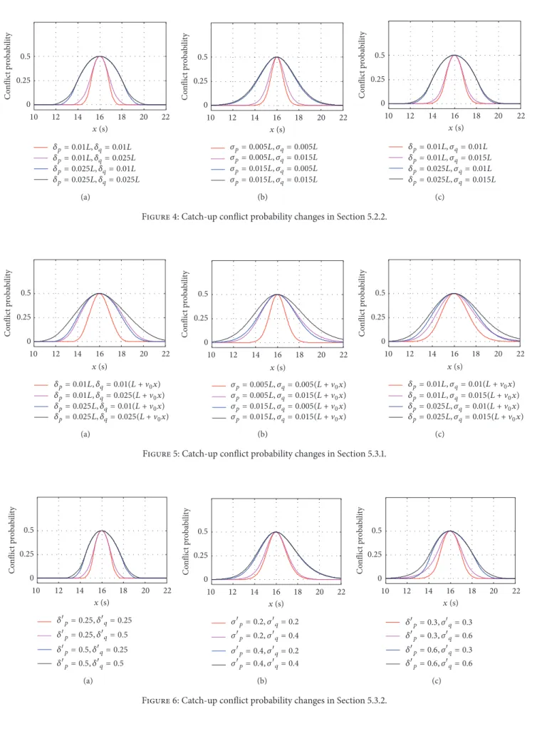
5.2.2. 𝜑(𝑡) Is Related to Travel Distance. 𝛿 and 𝜎 in (5) and

(6) change with travel distance. Here,𝐿 denotes the travel

distance from the start point to the current node. There are

three situations in which the distributions of𝜑_𝑝,28(𝑡), 𝜑_𝑞,28(𝑡),

𝜑_𝑝,29(𝑡), and 𝜑_𝑞,29(𝑡) are the same as shown in Table 1. The

(6)

10 12 14 16 18 20 22 0 0.25 0.5 x (s) C o nflic t p roba b ili ty p= 1, q= 0.25 p= 1, q= 1 p= 2.5, q= 0.25 p= 2.5, q= 1 (a) C o nflic t p roba b ili ty 0 0.25 0.5 10 12 14 16 18 20 22 x (s) p= 0.5, q= 0.25 p= 0.5, q= 0.5 p= 1, q= 0.25 p= 1, q= 0.5 (b) C o nflic t p roba b ili ty 0 0.25 0.5 10 12 14 16 18 20 22 x (s) p= 1, q= 0.25 p= 1, q= 0.5 p= 2, q= 0.25 p= 2, q= 0.5 (c)

Figure 3: Catch-up conflict probability changes in Section 5.2.1.

Table 3: Parameters in𝜑(𝑡).

𝜑_𝑝,28(𝑡), 𝜑_𝑝,29(𝑡) 𝜑_𝑞,28(𝑡), 𝜑_𝑞,29(𝑡)

A 𝛿 0.01𝐿 or 0.025𝐿 0.01(𝐿 + V₀𝑥) or 0.025(𝐿 + V₀𝑥)

B 𝜎 0.005𝐿 or 0.015𝐿 0.005(𝐿 + V0𝑥) or 0.015(𝐿 + V0𝑥)

C 𝛿/𝜎 0.01𝐿 or 0.025𝐿 0.01(𝐿 + V0𝑥) or 0.015(𝐿 + V0𝑥).

Simulated catch-up probabilities changing with𝑥 in the

three situations in Table 2 are shown in Figures 4(a), 4(b), and 4(c), respectively.

5.3. Conditions of Inference 4 Are Approximately Met

5.3.1. 𝜑(𝑡) Is Related to Travel Distance and 𝑥. For example,

the value of 𝛿_𝑞 or 𝜎_𝑞 in 𝜑_𝑞,28(𝑡) and 𝜑_𝑞,29(𝑡) is related to

𝐿 + V₀𝑥. In this case, it does not exactly meet the conditions

of Inference 4. However, if 𝜑_𝑞,28(𝑡) and 𝜑_𝑞,29(𝑡) do not

change significantly with 𝑥, the conditions of Inference 4

are met approximately. There are three situations in which

the distributions of𝜑_𝑝,28(𝑡), 𝜑_𝑞,28(𝑡), 𝜑_𝑝,29(𝑡), and 𝜑_𝑞,29(𝑡) are

the same as shown in Table 1. The parameters are shown in Table 3.

5.3.2. Travel Speed Is Random. When the probability density

function of travel speed has symmetric distribution, 𝜑(𝑡)

often is not strictly symmetric distribution. But if𝜑(𝑡) has

an approximately symmetric distribution and 𝜑_𝑞,28(𝑡) and

𝜑_𝑞,29(𝑡) change little with 𝑥, it can also be approximately

consistent with the conclusions of Inference 4.

Let the probability density function of travel speed be of

both uniform and normal distributions.𝜙(V) in (7) and (8)

are employed in𝜙_𝑝(V) and 𝜙_𝑞(V). For convenience, 𝛿󸀠_𝑝 and

𝜎󸀠_𝑝denote𝛿󸀠and𝜎󸀠in𝜙_𝑝(V), respectively, and 𝛿󸀠_𝑞and𝜎󸀠_𝑞

denote𝛿󸀠and𝜎󸀠in𝜙_𝑞(V), respectively. Similarly, according to

different combinations of travel speed in uniform and normal distributions, there are three situations shown in Table 4.

Table 4: Distributions and parameters in𝜙(V). 𝜙_𝑝(V) 𝜙_𝑞(V) A Distribution Uniform Uniform

𝛿󸀠 _{0.25 or 0.5} _{0.25 or 0.5}

B Distribution Normal Normal 𝜎󸀠 _{0.2 or 0.4} _{0.2 or 0.4}

C Distribution Uniform Normal 𝛿󸀠_/𝜎󸀠 _{0.3 or 0.6} _{0.3 or 0.6}

5.4. Discussions

5.4.1. Discussions about Section 5.2. In the situations in

Sections 5.2.1 and 5.2.2,𝑥₀ = 𝑡₁ − 𝑡₂ = 𝑡₃ − 𝑡₄ = 16 s.

In Figures 2 and 3, they are all symmetrical about𝑥 = 16 s;

when 𝑥 = 16 s, 𝑃(𝜍) = 𝑧(𝑥) reaches its maximum value

(0.5). In accordance with the cases in Sections 5.2.1 and 5.2.2,

monotonically increasing and decreasing intervals of𝑃(𝜍) =

𝑧(𝑥) obtained by simulations are shown in Tables 5 and 6, which are consistent with Inference 4.

In situation B of Sections 5.2.1 and 5.2.2, 𝑐_𝑝,28, 𝑐_𝑝,29,

𝑐_𝑞,28, 𝑐_𝑞,29 → −∞ and 𝑑_𝑝,28, 𝑑_𝑝,29, 𝑑_𝑞,28, 𝑑_𝑞,29 → +∞. In

situation C of Sections 5.2.1 and 5.2.2, 𝑐_𝑝,28, 𝑐_𝑝,29, 𝑑_𝑝,28,

and 𝑑_𝑝,29 are limited real numbers, 𝑐_𝑞,28, 𝑐_𝑞,29 → −∞,

𝑑_𝑞,28, 𝑑_𝑞,29→ +∞. In these four situations, 𝑆₂₈= (−∞, +∞),

𝑆₂₉= (−∞, +∞), and 𝑆_𝑘∪ 𝑆_𝑙= (−∞, +∞). Therefore, 𝑃(𝜍) =

(7)

0 0.25 0.5 C o nflic t p roba b ili ty 10 12 14 16 18 20 22 x (s) p= 0.01L, q= 0.01L p= 0.01L, q= 0.025L p= 0.025L, q= 0.01L p= 0.025L, q= 0.025L (a) 0 0.25 0.5 C o nflic t p roba b ili ty 10 12 14 16 18 20 22 x (s) p= 0.005L, q= 0.005L p= 0.005L, q= 0.015L p= 0.015L, q= 0.005L p= 0.015L, q= 0.015L (b) 0 0.25 0.5 C o nflic t p roba b ili ty 10 12 14 16 18 20 22 x (s) p= 0.01L, q= 0.01L p= 0.01L, q= 0.015L p= 0.025L, q= 0.01L p= 0.025L, q= 0.015L (c)

0 0.25 0.5 C o nflic t p roba b ili ty 10 12 14 16 18 20 22 x (s) p= 0.01L, q= 0.01(L + 0x) p= 0.01L, q= 0.025(L + 0x) p= 0.025L, q= 0.01(L + 0x) p= 0.025L, q= 0.025(L + 0x) (a) 0 0.25 0.5 C o nflic t p roba b ili ty 10 12 14 16 18 20 22 x (s) p= 0.005L, q= 0.005(L + 0x) p= 0.005L, q= 0.015(L + 0x) p= 0.015L, q= 0.005(L + 0x) p= 0.015L, q= 0.015(L + 0x) (b) 0 0.25 0.5 C o nflic t p roba b ili ty 10 12 14 16 18 20 22 x (s) p= 0.01L, q= 0.01(L + 0x) p= 0.01L, q= 0.015(L + 0x) p= 0.025L, q= 0.01(L + 0x) p= 0.025L, q= 0.015(L + 0x) (c)

0 0.25 0.5 C o nflic t p roba b ili ty 10 12 14 16 18 20 22 x (s) p= 0.25, q= 0.25  p= 0.25, q= 0.5  p= 0.5, q= 0.25  p= 0.5, q= 0.5 (a) 0 0.25 0.5 C o nflic t p roba b ili ty 10 12 14 16 18 20 22 x (s) p= 0.2, q= 0.2  p= 0.2, q= 0.4 p= 0.4, q= 0.2  p= 0.4, q= 0.4 (b) 0 0.25 0.5 C o nflic t p roba b ili ty 10 12 14 16 18 20 22 x (s) p= 0.3, q= 0.3  p= 0.3, q= 0.6  p= 0.6, q= 0.3  p= 0.6, q= 0.6 (c)

(8)

Table 5:𝑥’s intervals of 𝑃(𝜍) = 𝑧(𝑥) in situation A of Section 5.2.1.

Monotonicity of interval 𝛿_𝑝= 1,𝛿_𝑞= 0.25 𝛿_𝑝= 1,𝛿_𝑞= 1 𝛿_𝑝= 2.5,𝛿_𝑞= 0.25 𝛿_𝑝= 2.5,𝛿_𝑞= 1

Increasing [14.75, 16] [14, 16] [13.25, 16] [12.5, 16]

Decreasing [16, 17.25] [16, 18] [16, 18.75] [16, 19.5]

Monotonicity of interval 𝛿_𝑝= 0.01𝐿, 𝛿_𝑞= 0.01𝐿 𝛿_𝑝= 0.01𝐿, 𝛿_𝑞= 0.025𝐿 𝛿_𝑝= 0.025𝐿, 𝛿_𝑞= 0.01𝐿 𝛿_𝑝= 0.025𝐿, 𝛿_𝑞= 0.025𝐿 Increasing [14.2, 16] [13.45, 16] [12.25, 16] [11.5, 16] Decreasing [16, 17.8] [16, 18.55] [16, 19.75] [16, 20.5]

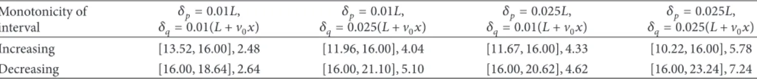
Table 7:𝑥’s intervals of 𝑃(𝜍) = 𝑧(𝑥) in situation A of Section 5.3.1. Monotonicity of interval 𝛿_𝑝= 0.01𝐿, 𝛿𝑞= 0.01(𝐿 + V0𝑥) 𝛿_𝑝= 0.01𝐿, 𝛿𝑞= 0.025(𝐿 + V0𝑥) 𝛿_𝑝= 0.025𝐿, 𝛿𝑞= 0.01(𝐿 + V0𝑥) 𝛿_𝑝= 0.025𝐿, 𝛿𝑞= 0.025(𝐿 + V0𝑥) Increasing [13.52, 16.00], 2.48 [11.96, 16.00], 4.04 [11.67, 16.00], 4.33 [10.22, 16.00], 5.78 Decreasing [16.00, 18.64], 2.64 [16.00, 21.10], 5.10 [16.00, 20.62], 4.62 [16.00, 23.24], 7.24

Monotonicity of interval 𝛿󸀠_𝑝= 0.25,𝛿󸀠_𝑞= 0.25 𝛿󸀠_𝑝= 0.25,𝛿󸀠_𝑞= 0.5 𝛿󸀠_𝑝= 0.5,𝛿󸀠_𝑞= 0.25 𝛿󸀠_𝑝= 0.5,𝛿󸀠_𝑞= 0.5 Increasing [14.24, 15.99], 1.75 [13.66, 15.99], 2.33 [13.12, 15.99], 2.87 [12.53, 15.99], 3.46 Decreasing [15.99, 17.72], 1.73 [15.99, 18.27], 2.28 [15.99, 19.18], 3.19 [15.99, 19.79], 3.8

[16, +∞), which is consistent with Figures 3(b), 3(c), 4(b), and 4(c).

In summary, the simulation results are consistent with the conclusions in Inference 4.

5.4.2. Discussions about Section 5.3. In Figures 5(a)–5(c),

the vertexes of the all curves are all (16.00, 0.50). From

the simulation results, the monotonically increasing and

decreasing intervals for 𝑃(𝜍) = 𝑧(𝑥) in situation A of

Section 5.3.1 are shown in Table 7. “[13.52, 16.00], 2.48” indicates that the increasing interval is [13.52 s, 16.00 s], and the length of this interval is 2.48 s. Although there are some differences among the lengths for increasing and decreasing intervals in each situation, it can be seen from Figure 5 that the catch-up probabilities are all approximately symmetrical

about𝑥 = 16 s.

In Figure 6(a), the vertexes of the four curves are all (15.99, 0.50). The monotonically increasing and decreasing

intervals for𝑃(𝜍) = 𝑧(𝑥) situation A of in Section 5.3.2 are

shown in Table 8. The indication of “[14.24, 15.99], 1.75” is the same as Table 7. It can be seen that the catch-up probabilities

are also approximately symmetrical about𝑥 = 16 s.

From Figures 5(b), 5(c), 6(b), and 6(c), it can be seen that, in each situation, the vertex of the catch-up probabilities is

approximately (16.00, 0.50); 𝑃(𝜍) = 𝑧(𝑥) is approximately

symmetrical about 𝑥 = 16 s; 𝑃(𝜍) = 𝑧(𝑥) monotonically

increases in (−∞, 16] and decreases in [16, +∞),

approxi-mately.

In summary, the probabilities of catch-up conflict changes in Section 5.3 are similar to the conclusions of Inference 4.

5.5. Simulation Conclusions and Time Window Setting. From

simulation results of catch-up conflict probability, it is known that the catch-up conflict probability reaches its maximum

when 𝑥 = 𝑥₀. When 𝑥 gradually decreases or increases

from𝑥₀, the catch-up conflict probability gradually decreases.

At last, the catch-up conflict probability is 0, or is close to 0. These probability features of AGV catch-up conflicts provide references for time window setting of the dynamic adjustment under uncertain travel time.

In the dynamic adjustment as detailed in Section 4, it is necessary to calculate the time windows. However, it is complicated to calculate them precisely according to Sec-tion 2. In contrast, it is simple and practical to apply Inference 4 and simulation conclusions of Section 5 to approximate calculation of time windows in AGVs operation. This feasible and beneficial strategy is as follows: for the link with “𝑃(𝜍) >

𝑇_ccp” after path preplanning, the corresponding𝑥 is initially

recorded. And then the𝑥 which makes |𝑥−𝑥₀| be the

histori-cal maximum is set as𝑥_𝑚, followed by the corresponding time

window[𝑥₀− |𝑥_𝑚− 𝑥₀|, 𝑥₀+ |𝑥_𝑚− 𝑥₀|]. Finally, in the process

of path replanning, if𝑥 is in the range [𝑥₀−|𝑥_𝑚−𝑥₀|, 𝑥₀+|𝑥_𝑚−

𝑥0|], logistics manager can determine that the corresponding

path is unacceptable (because of “𝑃(𝜍) > 𝑇ccp,” which can

be seen from Inference 4 and simulation conclusions of Section 5). Else, calculate the catch-up probability according

to Section 2. After the calculation, if “𝑃(𝜍) > 𝑇_ccp” still holds,

update𝑥_𝑚 and the corresponding time window. Although

this strategy cannot obtain the precise time windows at once, it is very favorable for AGV transportation systems since high time savings and improved efficiency encourage logistics

(9)

Table 9: Comparisons of adjustment effectiveness. Adjustment strategy _{“𝑃(𝜍) > 𝑇}Number of

ccp” Maximum conflict probability Average conflict probability Number of conflicts Average travel time Sensor detection 23 0.43 0.24 13 46.58 Conflict probability 0 0.23 0.13 2 38.17

managers to implement effectively. Therefore, this strategy is employed in Section 6.

6. Simulation on Dynamic Adjustment

The dynamic adjustment in Section 4 is verified by ten AGVs at an automated container terminal as shown in Figure 1.

The priority of AGVs is set as AGV₁ > AGV₂ > ⋅ ⋅ ⋅ >

AGV₁₀.𝑇_ccp = 0.25, which is half of the maximum of the

probability of catch-up conflict. The design speeds of AGVs are all 5 m/s, and the departure times of AGVs are random

values in [0 s, 10 s]. The starting nodes and final nodes are

random in quayside cranes and yard cranes. The probability density functions for times AGVs passing through nodes

are related to travel distance and 𝑥, and they are random

probability density functions in Sections 5.2 and 5.3. The data about catch-up conflicts of AGVs are shown in Table 9.

The data in the second row of Table 9 are referencing AGVs which avoid conflict only by sensor detection. In this mode, AGVs with low priority slow down or wait once con-flicts happen, and no dynamic adjustment is executed. The data in the third row of Table 9 are with reference to AGVs with dynamic adjustment detailed in Section 4. From

Fig-ure 1, it can be seen that some events of “𝑃(𝜍) > 𝑇_ccp” might

occur in the process of the dynamic adjustment, although

“𝑃(𝜍) > 𝑇_ccp” can be avoided after the dynamic adjustment.

Here, in the third row of Table 9, “Number of ‘𝑃(𝜍) > 𝑇_ccp’”

is the number of “𝑃(𝜍) > 𝑇_ccp” after the dynamic adjustment.

“Number of conflicts” is the number of catch-up conflicts that have occurred after the dynamic adjustment.

From Table 9, it can be observed that the number of

“𝑃(𝜍) > 𝑇ccp,” maximum conflict probability, average conflict

probability, number of conflicts, and average travel time of AGVs adjustment strategy based on conflict probability are quite smaller than those of AGVs adjustment strategy based on sensor detection.

The number of “𝑃(𝜍) > 𝑇_ccp” about AGVs adjustment

strategy based on conflict probability is 0, whereas the number of catch-up conflicts is more than 0. This is because

the situation in which𝑃(𝜍) ≤ 𝑇_ccphas not been dealt with in

dynamic adjustment.

Although the catch-up conflict cannot be eliminated completely in the execution of the dynamic adjustment strategy based on conflict probability, the number of conflicts has been greatly reduced. Such few potential conflicts will not cause serious problems in AGVs, because AGVs with low priorities can slow down or wait to avoid conflicts.

In brief, the dynamic adjustment based on conflict prob-ability is superior to the traditional adjustment based on detection using sensors. The proposed method lowers the frequency of control action and brings higher efficiency and

service ability of AGVs. The proposed method is suitable for the adjustment of path planning with uncertain travel time and has a high accuracy and practicability.

7. Conclusion

Travel time is crucial for the execution of transportation tasks. However, travel time uncertainty is one of the main defects of the loading and unloading operations often used in AGVs. This uncertainty affects AGV conflict and inevitably increases the variability in automated logistics systems. Higher travel time uncertainty leads to more difficult and complex path planning for AGVs.

To meet the demands of practical applications, this work considers the travel time uncertainty of AGVs, studies the impact of travel time uncertainty on AGV catch-up conflict, and designs the dynamic adjustment based on conflict proba-bility for AGVs. The probaproba-bility features of catch-up conflicts and the performances of the associated dynamic adjustment are simulated and validated for AGVs at an automated container terminal. The simulation results show that the con-clusions proposed in this work are correct, and the dynamic adjustment is effective. Moreover, the findings of the present work provide theoretical and decision-making bases for the improvement of automated logistics systems efficiency.

In the future, related work in different areas will be extended. First, the impact of other uncertainties, such as task arrival time and task assignment, on AGV conflict will be analyzed and verified in real automated logistics systems. Second, intelligent algorithms based on conflict probability for AGVs conflict-free path planning under uncertain envi-ronments will be designed.

Appendix

Proof of Theorem 1. ∵ 𝑔₁(𝑥) is symmetric about point

(𝑥₀, 0.5). ∴ 𝑔₁(𝑥₀+ Δ𝑥 ) + 𝑔₁(𝑥₀− Δ𝑥 ) = 2𝑔₁(𝑥₀) = 1. Similarly, 𝑔₂(𝑥₀+ Δ𝑥 ) + 𝑔₂(𝑥₀− Δ𝑥 ) = 1. From (3),𝑧(𝑥) = 𝑔₁(𝑥) + 𝑔₂(𝑥) − 2𝑔₁(𝑥) ⋅ 𝑔₂(𝑥). Thence,𝑧(𝑥₀+Δ𝑥) = 𝑔₁(𝑥₀−Δ𝑥)+𝑔₂(𝑥₀−Δ𝑥)−2𝑔₁(𝑥₀− Δ𝑥)𝑔2(𝑥0− Δ𝑥 ) = 𝑧(𝑥0− Δ𝑥 ).

Therefore,𝑃(𝜍) = 𝑧(𝑥) is symmetric about 𝑥 = 𝑥₀.

In addition,𝑧(𝑥₀) = 𝑔₁(𝑥₀) + 𝑔₂(𝑥₀) − 2𝑔₁(𝑥₀) ⋅ 𝑔₂(𝑥₀) =

0.5.

Then, Theorem 1 has been proven.

Proof of Inference 2.

Case 1. Both𝑔₁(𝑥) and 𝑔₂(𝑥) monotonically increase; then

𝑔₁(𝑥₁) < 𝑔₁(𝑥₂) ≤ 0.5 and 𝑔₂(𝑥₁) < 𝑔₂(𝑥₂) ≤ 0.5 when

(10)

From (3), 𝑧(𝑥₁) − 𝑧(𝑥₂) < 2𝑔₁(𝑥₂)[𝑔₂(𝑥₂) − 𝑔₂(𝑥₁)] +

𝑔₂(𝑥₁) − 𝑔₂(𝑥₂) ≤ 0.

Therefore,𝑃(𝜍) = 𝑧(𝑥) is an increasing function when

𝑥 ≤ 𝑥₀. From Theorem 1,𝑃(𝜍) is symmetric about 𝑥 = 𝑥₀.

Therefore,𝑃(𝜍) is a decreasing function when 𝑥 > 𝑥₀.

Case 2. Both𝑔₁(𝑥) and 𝑔₂(𝑥) monotonically decrease, then

𝑔₁(𝑥₁) < 𝑔₁(𝑥₂) ≤ 0.5 and 𝑔₂(𝑥₁) < 𝑔₂(𝑥₂) ≤ 0.5 when

𝑥1 > 𝑥2 ≥ 𝑥0. Similar to Case 1, it can be derived that𝑃(𝜍) is

an increasing function when𝑥 > 𝑥₀.

Therefore, Inference 2 has been proven.

Proof of Theorem 3. (1)∵ 𝜑_𝑝,𝑘(𝑡) and 𝜑_𝑞,𝑘(𝑡) are symmetric

about𝑡 = 𝑡₁and𝑡 = 𝑡₂, respectively.

∴ 𝐹_𝑝,𝑘(𝑡₁) = 𝐹_𝑞,𝑘(𝑡₂) = 0.5, 𝐹_𝑝,𝑘(𝑡), and 𝐹_𝑞,𝑘(𝑡₂) are

symmetric about points (𝑡₁, 0.5) and (𝑡₂, 0.5), respectively; the

probability density function of𝑡_𝑞,𝑘+ 𝑥 is 𝜑_𝑞,𝑘(𝑡 − 𝑥), which is

symmetric about𝑡 = 𝑡₂+ 𝑥.

∴ 𝑔(𝑥) = ∫_−∞+∞𝜑_𝑞,𝑘(𝜏 − 𝑥)𝐹_𝑝,𝑘(𝜏)𝑑𝜏.

Let𝑥₀= 𝑡₁− 𝑡₂; then𝑔(𝑥₀) is shown in

𝑔 (𝑥₀) = ∫+∞ −∞ 𝜑𝑞,𝑘(𝜏 − 𝑡1+ 𝑡2) 𝐹𝑝,𝑘(𝜏) 𝑑𝜏. (A.1) Let𝑢(𝜏) = 𝜑_𝑞,𝑘(𝜏 − 𝑡₁+ 𝑡₂)𝐹_𝑝,𝑘(𝜏); then 𝑢(𝑡₁− Δ𝑡) = 𝜑_𝑞,𝑘(𝑡₂− Δ𝑡)𝐹_𝑝,𝑘(𝑡₁− Δ𝑡), ∴ 𝑢(𝑡₁− Δ𝑡) + 𝑢(𝑡₁+ Δ𝑡) = 𝜑_𝑞,𝑘(𝑡₂+ Δ𝑡) ∴ 𝑔(𝑥₀) = ∫_𝑡+∞ 2 𝜑𝑞,𝑘(𝑡)𝑑𝑡 = 0.5. (2) From (A.1),𝑔(𝑥₀− Δ𝑥 ) + 𝑔(𝑥₀+ Δ𝑥 ) = ∫_−∞+∞[𝜑_𝑞,𝑘(𝜏 − 𝑥₀+ Δ𝑥 ) + 𝜑_𝑞,𝑘(𝜏 − 𝑥₀− Δ𝑥)]𝐹_𝑝,𝑘(𝜏)𝑑𝜏. Let 𝜓(𝜏) = 𝜑_𝑞,𝑘(𝜏 − 𝑥₀+ Δ𝑥 ) + 𝜑_𝑞,𝑘(𝜏 − 𝑥₀− Δ𝑥 ) and 𝜅(𝜏) = 𝜓(𝜏)𝐹_𝑝,𝑘(𝜏). Then,𝑔(𝑥₀− Δ𝑥 ) + 𝑔(𝑥₀+ Δ𝑥 ) = ∫_−∞+∞𝜅(𝑡)𝑑𝑡. In addition,𝜓(𝑡₁−Δ𝑡) = 𝜑_𝑞,𝑘(𝑡₂−Δ𝑡+Δ𝑥)+𝜑_𝑞,𝑘(𝑡₂−Δ𝑡− Δ𝑥), ∴ 𝜅(𝑡₁−Δ𝑡)+𝜅(𝑡₁+Δ𝑡) = 2𝐹_𝑝,𝑘(𝑡₁)𝜓(𝑡₁+Δ𝑡) = 𝜓(𝑡₁+Δ𝑡). ∴ ∫₀+∞𝜅(𝑡₁−Δ𝑡)𝑑(Δ𝑡)+∫₀+∞𝜅(𝑡₁+Δ𝑡)𝑑(Δ𝑡) = ∫₀+∞𝜙(𝑡₁+ Δ𝑡)𝑑(Δ𝑡). ∴ 𝑔(𝑥₀− Δ𝑥 ) + 𝑔(𝑥₀+ Δ𝑥 ) = ∫_𝑡+∞ 1 𝜓(𝑡)𝑑𝑡, ∫ +∞ 𝑡1 𝜑𝑞,𝑘(𝜏 − 𝑥₀+ Δ𝑥)𝑑𝜏 = 1 − 𝐹_𝑞,𝑘(𝑡₂+ Δ𝑥 ). Similarly,∫_𝑡+∞ 1 𝜑𝑞,𝑘(𝜏 − 𝑥0− Δ𝑥)𝑑𝜏 = 1 − 𝐹𝑞,𝑘(𝑡2− Δ𝑥 ), ∴ 𝑔(𝑥₀− Δ𝑥 ) + 𝑔(𝑥₀+ Δ𝑥 ) = 1 = 2𝑔(𝑥₀).

In summary,𝑃(𝑡_𝑝,𝑘 ≤ 𝑡_𝑞,𝑘+ 𝑥 ) is symmetric about point

(𝑡₁− 𝑡₂, 0.5).

Proof of Inference 4. Let𝑆_𝑘∩ 𝑆_𝑙 = [𝑒, 𝑓]; then [𝑒, 𝑓] ⊆ [𝑎, 𝑏].

From Theorem 3,𝑃(𝑡_𝑝,𝑘≤ 𝑡_𝑞,𝑘+ 𝑥 ) = 𝑔₁(𝑥) and 𝑃(𝑡_𝑝,𝑙≤ 𝑡_𝑞,𝑙+

𝑥 ) = 𝑔₂(𝑥) are both symmetric about the point (𝑡₁− 𝑡₂, 0.5).

And then from Theorem 1,𝑃(𝜍) = 𝑧(𝑥) is symmetric about

𝑥₀= 𝑡₁− 𝑡₂, and𝑧(𝑥₀) = 0.5. Then 𝑔₁(𝑥) is { { { { { { { { { 0, 𝑥 ≤ 𝑐_𝑝,𝑘− 𝑑_𝑞,𝑘 monotonically increasing, 𝑥 ∈ [𝑐_𝑝,𝑘− 𝑑_𝑞,𝑘, 𝑑_𝑝,𝑘− 𝑐_𝑞,𝑘] 1, 𝑥 ≥ 𝑑𝑝,𝑘− 𝑐𝑞,𝑘, 𝑔₂(𝑥) is { { { { { { { { { 0, 𝑥 ≤ 𝑐_𝑝,𝑙− 𝑑_𝑞,𝑙 monotonically increasing, 𝑥 ∈ [𝑐_𝑝,𝑙− 𝑑_𝑞,𝑙, 𝑑_𝑝,𝑙− 𝑐_𝑞,𝑙] 1, 𝑥 ≥ 𝑑_𝑝,𝑙− 𝑐_𝑞,𝑙. (A.2)

From Theorem 3,𝑥₀= 𝑡₁− 𝑡₂is the midpoint of𝑆_𝑘= [𝑐_𝑝,𝑘−

𝑑_𝑞,𝑘, 𝑑_𝑝,𝑘−𝑐_𝑞,𝑘] and 𝑆_𝑙= [𝑐_𝑝,𝑙−𝑑_𝑞,𝑙, 𝑑_𝑝,𝑙−𝑐_𝑞,𝑙]. Therefore, 𝑆_𝑘 ⊆ 𝑆_𝑙

or𝑆_𝑘⊇ 𝑆_𝑙.

From Inference 2,𝑃(𝜍) = 𝑧(𝑥) increases when 𝑥 ∈ [𝑒, 𝑥₀],

while 𝑃(𝜍) = 𝑧(𝑥) decreases when 𝑥 ∈ [𝑥₀, 𝑓]. If 𝑥 ∈

(−∞, 𝑎] ∪ [𝑏, +∞), then 𝑔₁(𝑥) = 𝑔₂(𝑥) = 0 and 𝑧(𝑥) = 0.

Here, the relationships between𝑆_𝑘and𝑆_𝑙are discussed for

three cases.

Case 1.𝑆_𝑘 = 𝑆_𝑙; then𝑆_𝑘∪ 𝑆_𝑙= 𝑆_𝑘∩ 𝑆_𝑙(that is,[𝑒, 𝑓] ⊆ [𝑎, 𝑏]); ∴ Formula (11) is true.

Case 2 (𝑆_𝑘 ⊂ 𝑆_𝑙). If𝑥 ∈ [𝑎, 𝑒], then 𝑔₂(𝑥) ∈ (0, 1), 𝑔₁(𝑥) =

0, and 𝑧(𝑥 ) = 𝑃(𝜍) = 𝑔₂(𝑥) > 0; ∴ 𝑔₂(𝑥) and 𝑧(𝑥)

are monotonically increasing; if 𝑥 ∈ [𝑓, 𝑏], then 𝑔₂(𝑥) ∈

(0, 1), 𝑔₁(𝑥) = 1, and 𝑧(𝑥) = 𝑃(𝜍) = 1 − 𝑔₂(𝑥) > 0.

Therefore,𝑔₂(𝑥) is monotonically increasing, while 𝑧(𝑥) is

monotonically decreasing. Therefore, Formula (11) is true.

Case 3(𝑆_𝑘⊃ 𝑆_𝑙). Being similar to Case 2, Formula (11) is true

when𝑆_𝑘⊃ 𝑆_𝑙.

Therefore, Inference 4 has been proven.

Conflicts of Interest

The authors declare that they have no conflicts of interest.

Acknowledgments

This work was supported by the Ministry of Education of Humanities and Social Science Project (Grants nos. 15YJC630145 and 15YJC630059) and Natural Science Foun-dation of Shanghai Science and Technology Committee (Grant no. 15ZR1420200).

References

[1] M. Saidi-Mehrabad, S. Dehnavi-Arani, F. Evazabadian, and V. Mahmoodian, “An Ant Colony Algorithm (ACA) for solving

(11)

the new integrated model of job shop scheduling and conflict-free routing of AGVs,” Computers & Industrial Engineering, vol. 86, pp. 2–13, 2015.

[2] M. Zhang, R. Batta, and R. Nagi, “Modeling of workflow congestion and optimization of flow routing in a manufactur-ing/warehouse facility,” Management Science, vol. 55, no. 2, pp. 267–280, 2009.

[3] H. Fazlollahtabar, M. Saidi-Mehrabad, and E. Masehian, “Math-ematical model for deadlock resolution in multiple AGV scheduling and routing network: A case study,” Industrial Robot:

An International Journal, vol. 42, no. 3, pp. 252–263, 2015.

[4] N. Smolic-Rocak, S. Bogdan, Z. Kovacic, and T. Petrovic, “Time windows based dynamic routing in multi-AGV systems,” IEEE

Transactions on Automation Science and Engineering, vol. 7, no.

1, pp. 151–155, 2010.

[5] A. Hidalgo-Paniagua, M. A. Vega-Rodr´ıguez, and J. Ferruz, “Applying the MOVNS (multi-objective variable neighborhood search) algorithm to solve the path planning problem in mobile robotics,” Expert Systems with Applications, vol. 58, pp. 20–35, 2016.

[6] G. Zou, T. Li, and Y. Qin, “Automated Guide Vehicles Dynamic Scheduling Based on Annealing Genetic Algorithm,”

Telkom-nika, vol. 11, no. 5, pp. 2508–2515, 2013.

[7] C. Wei, Y. Asakura, and T. Iryo, “A probability model and sam-pling algorithm for the inter-day stochastic traffic assignment problem,” Journal of Advanced Transportation, vol. 46, no. 3, pp. 222–235, 2012.

[8] T. Zhang, W. A. Chaovalitwongse, and Y. Zhang, “Scatter search for the stochastic travel-time vehicle routing problem with simultaneous pick-ups and deliveries,” Computers & Operations

Research, vol. 39, no. 10, pp. 2277–2290, 2012.

[9] T. Van Woensel, L. Kerbache, H. Peremans, and N. Vandaele, “A queueing framework for routing problems with time-dependent travel times,” Journal of Mathematical Modelling and

Algorithms, vol. 6, no. 1, pp. 151–173, 2007.

[10] S. Shao, Z. Xia, G. Chen, and J. Zhang, “A new scheme of multi-ple automated guided vehicle system for collision and deadlock free,” in Proceedings of the IEEE International Conference on

Information Science & Technology, pp. 606–610, Washington, D.

C., USA, 2014.

[11] J. Zhang, W. H. Lam, and B. Y. Chen, “A stochastic vehicle routing problem with travel time uncertainty: trade-off between cost and customer service,” Networks and Spatial Economics, vol. 13, no. 4, pp. 471–496, 2013.

[12] J. H. Lee, B. H. Lee, and M. H. Choi, “A real-time traffic control scheme of multiple AGV systems for collision free minimum time motion: A routing table approach,” IEEE Transactions on

Systems, Man and Cybernetics, Part A: Systems and Humans, vol.

28, no. 3, pp. 347–358, 1998.

[13] Q. Li, J. T. Udding, and A. Y. Pogromsky, “Modeling and control of the AGV system in an automated container terminal,” in

Proceedings of the 30th IASTED Conference on Modelling, Iden-tification, and Control, AsiaMIC 2010, pp. 166–173, Thailand,

November 2010.

[14] K. Hoo-Lim, C. Ri, P. Tae-Jin, and R. Kwang-Ryel, “Dynamic Optimization of the Traffic Flow of AGVs in an Automated Container Terminal,” Journal of KIISE: Computing Practices and

Letters, vol. 16, no. 5, pp. 591–595, 2010.

[15] L. Chen, M. H. H`a, A. Langevin, and M. Gendreau, “Optimizing road network daily maintenance operations with stochastic ser-vice and travel times,” Transportation Research Part E: Logistics

and Transportation Review, vol. 64, pp. 88–102, 2014.

[16] P. Burnos, J. Gajda, Z. Marszałek et al., “Road Traffic Parameters Measuring System with Variable Structure,” Metrology and

(12)

Hindawi www.hindawi.com Volume 2018

Mathematics

Journal of Hindawi www.hindawi.com Volume 2018 Mathematical Problems in Engineering Applied Mathematics Hindawi www.hindawi.com Volume 2018

Probability and Statistics Hindawi

www.hindawi.com Volume 2018

Hindawi

www.hindawi.com Volume 2018

Mathematical PhysicsAdvances in

Complex Analysis

Journal of

Optimization

Journal of Hindawi www.hindawi.com Volume 2018 Hindawi www.hindawi.com Volume 2018 Engineering Mathematics International Journal of Hindawi www.hindawi.com Volume 2018 Operations Research Journal of Hindawi www.hindawi.com Volume 2018

Function Spaces

Abstract and Applied Analysis

Hindawi www.hindawi.com Volume 2018 International Journal of Mathematics and Mathematical Sciences Hindawi www.hindawi.com Volume 2018

Hindawi Publishing Corporation

http://www.hindawi.com Volume 2013 Hindawi www.hindawi.com

World Journal

Volume 2018 Hindawi

www.hindawi.com Volume 2018Volume 2018

Numerical Analysis

Advances inAdvances in Discrete Dynamics in Nature and Society

Hindawi www.hindawi.com Volume 2018 Hindawi www.hindawi.com Differential Equations International Journal of Volume 2018 Hindawi www.hindawi.com Volume 2018

Impact analysis of travel time uncertainty on AGV catch-up conflict and the associated dynamic adjustment

Research Article