How green is sugarcane ethanol?

Ensaios Econômicos

How green is sugarcane ethanol?

Marcelo Sant’Anna

Os artigos publicados são de inteira responsabilidade de seus autores. As

opiniões neles emitidas não exprimem, necessariamente, o ponto de vista da

Fundação Getulio Vargas.

EPGE Escola Brasileira de Economia e Finanças Diretor Geral: Rubens Penha Cysne

Vice-Diretor: Aloisio Araujo

Coordenador de Regulação Institucional: Luis Henrique Bertolino Braido

Coordenadores de Graduação: Luis Henrique Bertolino Braido & André Arruda Villela Coordenadores de Pós-graduação Acadêmica: Humberto Moreira & Lucas Jóver Maestri Coordenadores do Mestrado Profissional em Economia e Finanças: Ricardo de Oliveira Cavalcanti & Joísa Campanher Dutra

Sant’Anna, Marcelo

How green is sugarcane ethanol?/ Marcelo Sant’Anna – Rio de Janeiro : FGV,EPGE, 2019

53p. - (Ensaios Econômicos; 807) Inclui bibliografia.

How green is sugarcane ethanol?

Marcelo Sant’Anna

First draft: Nov/2015, This draft: July/2019

Abstract

Biofuels offer one approach for reducing carbon emissions in transportation. How-ever, the agricultural expansion needed to produce biofuels may endanger tropical forests. I use a dynamic model of land use to disentangle the roles played by agricul-tural expansion and yield increases in the supply of sugarcane ethanol in Brazil. The model is estimated using remote sensing (satellite) information of sugarcane activities. Estimates imply that, at the margin, 92% of new ethanol comes from increases in area and only 8% from increases in yield. Direct deforestation accounts for 12% of area ex-pansion. I further assess carbon emissions and deforestation implications from ethanol policies.

JEL: Q11, Q16, Q57

∗_{FGV EPGE - Escola Brasileira de Economia e Finanças, e-mail: marcelo.santanna@fgv.br. I am} grate-ful to Philip Haile and Steven Berry for invaluable advice and support in this project. I thank Kenneth Gillingham, Camilla Roncoroni, Lorenzo Magnolfi and numerous seminars and conferences participants. All errors are my own.

1

Introduction

In the past decade the world has seen an unprecedented debate on climate change, mainly about how to reduce emissions of CO2 and other greenhouse gases. Reduction of emissions is especially challenging in the transportation sector, which still relies heavily on fossil fuels.1 Biofuels are an attractive tool for reducing carbon emissions in transportation, as they can be blended with petroleum fuels in unmodified vehicles. This is an advantage of biofuels compared to other lower carbon alternatives for transportation, such as electric vehicles, as it does not require changes in the vehicle stock or the refueling infrastructure. However, the agricultural expansion needed to produce biofuels may endanger tropical forests or other nat-ural habitats and thus offset the alleged environmental benefits of fossil fuels substitution.2 This deforestation could be reduced if more biofuels are produced by increasing agricultural yields in existing growing areas.

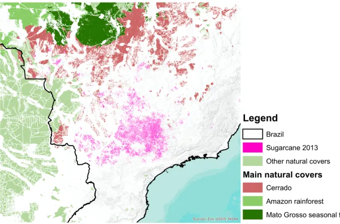
To assess the environmental benefits of biofuels, we need to understand the roles played by acreage expansion and yield increases as we move along the supply curve to meet the increased demand for biofuels feedstock. These issues are particularly important for Brazilian sugarcane ethanol, which accounts for 26% of the world ethanol supply in 2017. A large portion of Brazil is covered by tropical ecosystems, such as the Amazon rainforest, with important biodiversity and carbon storage. Figure 1 shows the remaining ecosystems in Brazil alongside existing sugarcane fields in 2013. Those ecosystems could be endangered by the expansion of farmland that would follow an increase in sugarcane ethanol demand.

In this paper, I disentangle the roles played by farmland expansion and agricultural yields in determining the supply of sugarcane ethanol in Brazil. I further estimate the effect of

1_{Transportation accounted for 23% of energy-related emissions in 2010 and transport}

demand is on the rise in the developing world (IPCC, 2014).

2_{The Intergovernmental Panel on Climate Change (IPCC) recognizes a lack of consensus}

on the role biofuels should play in climate change policies. The IPCC Fifth Assessment Report (IPCC, 2014) recommends support for biofuels be given on a case by case basis.

farmland expansion on forests and other untouched ecosystems.

The agronomic technology of sugarcane farming both guides my modeling and provides the means by which yields may respond to prices. Sugarcane is a semi-perennial crop, with declining expected yields over time until fields are replanted and yields restored. Replanting a field or planting sugarcane for the first time requires fixed land preparation investments that only pay off in future seasons, which makes optimal decisions forward-looking. The sugarcane growing technology gives a natural way in which prices can affect average yields through changes in the timing of replanting. By increasing the frequency of replanting, a farmer can boost average yields.

The most common types of biofuels policies, e.g., ethanol mandates, imply permanent shifts in the demand for feedstock used to produce biofuels. Given the fixed costs of land preparation, an increase in price perceived as permanent generates different incentives in terms of sugarcane planting and replanting than transitory price shocks. In this industry, such clean permanent price changes are hard to see in the data. My approach is to use variation in agricultural profitability and replanting patterns to estimate a model that allows me to disentangle the effects of permanent price changes on the intensive (yield) and extensive (acreage) margins.

I incorporate both adoption of sugarcane and replanting in a single dynamic model. In the model, farmers planting sugarcane must decide at every period either to replant their sugarcane fields or not. If they do not replant, expected yields decline next period. If they choose to replant, they pay a fixed replanting cost and sugarcane yields are restored. This feature makes this problem similar to optimal machine replacement (Rust, 1987).3 Farmers always have the option of switching away from sugarcane production to other uses. Meanwhile, farmers not planting sugarcane must decide at every period whether to plant sugarcane or not. Payoffs from both sugarcane and other uses depend on prices that are

3_{There is also an interesting parallel with optimal oil drilling (Kellogg (2014), Anderson}

allowed to evolve stochastically.

I estimate the model using a unique remote sensing dataset of sugarcane land use in Brazil from the CANASAT project (Rudorff et al., 2010). The project processes satellite images from Landsat to provide detailed maps of sugarcane field activity for the most important sugarcane producing region of Brazil. I complement this land use data with GAEZ/FAO high-resolution potential yield information and other detailed field level land characteristics. Given the sparsity of good transportation network in remote areas of Brazil, transportation costs are an important source of variation in agricultural profitability. Therefore, I model a quality-adjusted transportation network, which is used to measure the transportation cost to destination markets.

I use the model estimates to decompose the sugarcane supply elasticity into farmland expansion (extensive margin) and yield (intensive margin) components. I find a long-run yield elasticity of 0.32, comparable to what is believed an upper bound for most annual crops in developed countries.4 However, I find a value for the long-run acreage elasticity of 3.94, which is a different order of magnitude compared to the yield elasticity. The combined effects of acreage and yield translates into a high supply elasticity, which suggests small price effects from demand shifts. The high acreage to yield elasticity ratio I find means that, as we move along the supply curve, 92% of new ethanol comes from expansion in farmland and only 8% from yield increase that accrues from a faster replanting rate.

The high long-run acreage elasticity found here contrasts with existing measures of acreage price responses in the literature. Roberts and Schlenker (2013) measure short-run demand and supply elasticities for food crops and find inelastic demand and supply. Scott (2013a) estimates the acreage elasticity using a dynamic model and US land use data. He finds a higher long-run acreage elasticity once forward-looking behavior is taken into ac-count. However, the acreage elasticity found by Scott (2013a) is still an order of magnitude

4_{See Berry (2011), Scott (2013b) and Miao et al. (2015) for discussions on the potential}

lower than the acreage elasticity I find for sugarcane in Brazil. This difference can be due in part to the very active Brazilian agricultural frontier compared to the already consolidated American farmland. This highlights the danger of extrapolating measures of acreage elastic-ity from one country to another when evaluating land use changes. Using American numbers for long run acreage responses in Brazil would imply that 45% of new ethanol at the margin would come from yield increases. This would severely understate the environmental costs of biofuels policies as a smaller fraction of new ethanol would be coming from expansion in farmland.

The high-resolution nature of the data together with the estimated model allows me to make predictions about which types of land cover are affected by sugarcane expansion. Out of the total farmland expansion, 12% is predicted to be over forests and other types of natural cover, with the Cerrado ecosystem and the southern fringe of the Amazon rainforest being the most affected. Deforestation can be magnified by indirect land substitution as sugarcane takes over other cropland and pasture. The expansion of sugarcane in areas with previous agricultural use decreases the supply of other agricultural products and is expected to cause further expansion of farmland as the market re-equilibrates at a higher price level.

I use available empirical evidence to quantify these indirect effects in deforestation. In order to put this predicted deforestation in perspective, I balance the carbon released by direct and indirect deforestation and the carbon saved by replacing fossil fuels. I find that new ethanol “pays back” in terms of carbon in about 20 years. In contrast, corn ethanol produced in the US is expected to “pay back” in 167 years (Searchinger et al., 2008). Currently there is no consensus about payback times for sugarcane ethanol. Estimates of the sugarcane ethanol carbon payback time vary from 4 to more than 100 years in the scientific literature, depending on the type of land cover affected (Elshout et al. (2015), Gibbs et al. (2008), Fargione et al. (2008)). In this paper, I compute a carbon payback time that brings together the economics of land use and the current scientific knowledge about emissions from land use change.

As an illustrative policy experiment, I discuss the implications of current U.S. Renewable Fuel Standard (RFS) for land use in Brazil. The current standard assigns a total of 5 billion gallons in the Advanced Biofuels (ABF) category that need not be met by cellulosic biofuels. This is equivalent to about only 3% of the U.S. annual gasoline consumption. As of now, Brazilian sugarcane ethanol is the only viable large scale alternative to fill the ABF mandate. I find that a 5 billion gallons shift in the market demand for sugarcane ethanol would imply a modest 2.6% price increase, but about 4,500 sq. km in direct deforestation.

This is not the first study to investigate the implications of ethanol policies in the context of Brazilian sugarcane ethanol (e.g., De Gorter et al. (2013), Elobeid and Tokgoz (2008), Lasco and Khanna (2010) and Nagavarapu (2010)). Other studies in the literature use mainly static general equilibrium to evaluate the effects of policies in the markets for sugar and ethanol using supply elasticities derived from short-run responses to prices. An exception is Nagavarapu (2010), which estimates a static general equilibrium model for land use and labor allocation in the sugarcane industry in Brazil using micro level data on the worker decision, but aggregate data on land use.

The rest of the paper is organized as follows. Section 2 presents a short background of the sugarcane industry in Brazil. Section 3 describes in more detail the land use model. Section 4 presents the data and some descriptive analysis. Section 5 discusses the model estimation. Counterfactuals are discussed in Section 6. Section 7 concludes.

2

Industry background

Sugarcane has long history in Brazil, dating back to colonial times. Once sugar was the most important export commodity in the country, but its importance for the Brazilian economy has faded away over time. In the aftermath of the seventies oil shocks, a government program (PROALCOOL) was created to foster the use of sugarcane ethanol as a replacement for gasoline. Large scale production of sugarcane ethanol has been in place since then. In the

past decade, the emergence of flex-fuel vehicles has given a new boost to the sugarcane ethanol industry.

Sugarcane has been historically grown close to the coast in Southeast and Northeast Brazil. Today, more than half of sugarcane in Brazil is produced in the State of São Paulo, where physical conditions are ideal for sugarcane growing. In general, suitable conditions for sugarcane include a warm and rainy growing season and a cooler and drier harvest season. The harvest season in the region studied here goes from April to November, depending on the location and the varieties used. Sugarcane is a semi-perennial crop, which means that after plants are cut, if the roots are untouched, a ratoon or stubble crop will follow. However, yields for the ratoon crop are expected to be lower every time this process is repeated (Crago et al. (2010), Macedo et al. (2008)). For this reason, periodically the field must be replanted so that yields can be restored. Agriculture manuals recommend replanting roughly every 5 years.

After harvest, sugarcane is transported to a nearby mill, which is usually located at close proximity to sugarcane fields. Sugarcane is bulky, so it would be uneconomical to ship cane long distances for milling. Moreover the sugars in the cane deteriorate quickly after it has been cut, so generally mills are not more than 40 km away from source fields. At the mill the sugarcane is crushed and the resulting liquid is either fermented to produce ethanol or processed to produce sugar. Modern mills are also thermal electricity generators. They produce electricity by burning leftovers from the crushing process. This innovation significantly helped the sugarcane ethanol energy balance (Macedo et al., 2008). Although, there are constant improvements in the milling process, like electricity generation from fibrous materials, the milling technology is well known. There is an active market of equipment and machinery for mills and I know of no technological barriers to entry.

Most modern mills can produce both sugar or ethanol and switch production according to market conditions. This technological feature implies that under perfect competition the price for sugar and ethanol should follow closely together in the medium-run (De Gorter

et al., 2013). I consider therefore an unified sugarcane final products market in my analysis, that includes both sugar and ethanol as final outputs. As discussed above, most of the controversy regarding sugarcane ethanol is on aspects related to land use and yields and not on emissions accruing from the industrial processes, as those are well understood.

3

Model

The unit of analysis is a field indexed by i, which is managed by a profit maximizing farmer. In each year, t, farmers must make a decision regarding land use for the next season. This decision is denoted by qit. If farmers are not planting sugarcane, qit ∈ {plant, stay}, i.e., they

can either plant sugarcane or keep their fields in another economic use. For farmers already planting sugarcane, qit ∈ {replant, keep, out}, i.e., they can (i) replant the sugarcane fields,

(ii) keep the same plants for next season or (iii) switch land use to another activity.

I denote by ait ∈ {0, 1, . . . , ¯a} the state of fields regarding its sugarcane use. If ait = 0,

the field is not in sugarcane use, while if ait≥ 1, the field is in sugarcane use and ait denotes

the sugarcane field age. I denote by wit ∈ W the exogenous state vector, with information

on prices of sugarcane products and alternative crops, land characteristics, transportation costs and distance to existing sugarcane fields. Finally, there is a state vector εit∈ R5 which

farmers observe but not the econometrician. The flow payoff is given by:

Π(ait, wit, qit, εit; θ) = π(ait, wit, qit; θ) + εit(qit), (1)

where π(ait, wit, qit; θ) is a function that depends only on observed state variables and on a

vector of parameters to be estimated, θ. Equation 1 makes it clear that for each choice qit,

there is a different associated unobserved state εit(qit).

payoff is given by: π(0, wit, qit; θ) =          δrit, if qit = stay, −ΨE(hi, dit; θ), if qit = plant. (2)

The return index ritcaptures the payoff from non sugarcane uses. I defer the discussion about

how the return index rit is constructed to Section 4.4. If farmers choose to stay in other use, qit = stay, then ait+1 = ait = 0. The fixed cost of sugarcane planting ΨE(hi, dit; θ) depends

on the previous land use, hi, and on the distance between the field and the closest existing

sugarcane field at the time dit. As discussed in the previous section, due to cane bulkiness,

sugarcane fields are usually not more than 40 km away from a mill. Therefore, ditproxies for

mill proximity and ΨE(·; θ) captures the cost of moving the agro-industrial complex (mills

and other specific infra-structure) further into the agriculture frontier. The higher cost of planting sugarcane in land farther away from existing sugarcane activities helps to explain the sluggish pattern of sugarcane expansion we see in the data. Note that if farmers decide to plant sugarcane, they reap no sugarcane in the immediate season following their decision. Using the most common plant varieties, after planting (or replanting) sugarcane fields take one and a half years to be ready for harvest. If farmers choose to plant sugarcane, qit= plant,

then ait+1 = 1.

The flow payoff for fields in sugarcane use, ait ≥ 1, is given by:

π(ait, wit, qit; θ) =                    (ps_t − tci)κγait−1yis+ x0iβ, if qit = keep, −ΨR, if qit = replant, δrit− ΨA, if qit = out. (3)

If farmers keep the sugarcane fields, their next expected yields are given by the sugarcane potential yields for field i, ys

i, adjusted by the exponential decay in sugarcane productivity

to final product. Variables ps

t and tci denote, respectively, the final product price and

trans-portation cost to port. The vector xi keeps track of land specific characteristics, such as

climate, elevation, slope and soil type. Those characteristics should affect harvest and up-keep costs (e.g., the amount of fertilizer used), so they are allowed to shift the period return from sugarcane through the term x0_iβ. Naturally, physical land characteristics in xi should

also influence sugarcane yields. However, the effect of those variables in expected yields is assumed to be fully captured by the potential yield measure y_is.5 Finally, if qit = keep, the

sugarcane field ages in the next season, i.e., ait+1 = min{ait + 1, ¯a}. If farmers decide to

replant, they pay a fixed cost ΨR. Analogously to sugarcane planting, there are no

sugar-cane related payoffs in the next season. The replanting decision resets field age: ait+1 = 1.

Switching to other uses gives the farmer the return from those other uses, at a fixed land conversion cost ΨA, and sets ait+1 = 0.

In industry discussions, local weather shocks were usually listed as the most important factor affecting replanting decisions after sugarcane field age. Particularly bad weather may increase the costs of the agricultural operation necessary for field replanting as well as per period field upkeep costs. The effects of these weather shocks are captured by the state variable εit(qit). Moreover, replanting decisions may not always coincide with the optimal

decision from the agronomic point of view. For instance, mills must make sure they have a steady supply of sugarcane, therefore all source fields cannot replant at the same time. In this sense, εit(qit) captures the additional noise introduced by other operational concerns.

Assumption 1. The unobserved state variables, ε_it(q), are independently and identically

distributed over fields and time.

5_{In the model, I assume farmers use a fixed amount of inputs that gives the maximum}

attainable yield ys

i. Input choice is an additional margin farmers could use to increase yields.

Empirical evidence for high intensity agriculture suggests this margin should be small. For instance, Scott (2013b) finds an upper bound for the yield elasticity of 0.05 from changes in fertilizer use.

Assumption 2. The evolution of the exogenous state variables w is not affected by farmers decisions and ε, i.e., Fwit+1|qit,εit,wit = Fwit+1|wit.

Assumption 1 is standard in the dynamic discrete choice literature. Assumption 2 embeds two important underlying features. First, it implies that farmers are price takers, a reason-able assumption for agricultural products markets. Second, it implies that choice specific unobservables ε do not change expectations about the evolution of w.

I assume farmers discount future cash flows using a fixed discount rate ρ < 1. Farmers choose qit every period conditional on (ait, wit, εit) in order to maximize the sum of future

discounted flow payoffs:

max qit E   ∞ X j=0

ρjΠ(ai,t+j, wi,t+j, qi,t+j, εi,t+j; θ)|ait, wit, εit



.

I rewrite below the dynamic optimization problem faced by farmers in the recursive Bellman formulation. In a non sugarcane state, a farmer has two options: leave the land in other use or convert the land to sugarcane. Therefore, the value function at ait= 0 is

Vθ(0, wit, εit) = max {π(0, wit, stay; θ) + εit(stay) + ρE [Vθ(0, wit+1, εit+1)|wit] ,

π(0, wit, plant; θ) + εit(plant) + ρE [Vθ(1, wit+1, εit+1)|wit]} . (4)

At 1 ≤ ait≤ ¯a , which are the productive sugarcane field states, the farmer can either keep

the current field, replant or switch to other use. In this case, the value function is

Vθ(ait, wit, εit) = max {π(ait, wit, keep; θ) + εit(keep) + ρE [Vθ(min{ait+ 1, ¯a}, wit+1, εit+1)|wit] , π(ait, wit, replant; θ) + εit(replant) + ρE [Vθ(1, wit+1, εit+1)|wit] ,

Assumptions 1 and 2 imply the expected continuation value does not depend on the present unobserved state εit. Moreover, by Assumption 2, current choices do not alter the

distribution of wit+1 conditional on wit. Let vθ(ait, wit, qit) be the deterministic component

of each choice’s value, that is,

vθ(ait, wit, qit) = π(ait, wit, qit; θ) + ρE [Vθ(ait+1(ait, qit), wit+1, εit+1)|wit] ,

where ait+1(ait, qit) denotes the deterministic age transition given current age and choice.

The optimal choice, or policy function, is given by:

q?_θ(ait, wit, εit) = arg max

q vθ(ait, wit, q) + εit(q).

Since εit is unobserved to the econometrician, given observed state variables and

param-eters θ, we are not able to precisely determine the optimal choice. We can only recover a conditional choice probability (CCP) given the unobserved state distribution:

Pr(q|ait, wit; θ) =

Z

1{vθ(ait, wit, q) + εit(q) ≥ vθ(ait, wit, q0) + εit(q0) for all q0}dG(εit).

Assumption 3. εit(q) is independently and identically distributed across alternatives with type 1 extreme value distribution.

Assumption 3 implies the CCP has the usual logit form:

Pr(q|ait, wit; θ) =

vθ(ait, wit, q)

P

q0v_θ(a_it, w_it, q0)

. (6)

The CCP is the basic building block of the likelihood approach I use to estimate the model’s vector of parameters θ. Aguirregabiria and Mira (2010) provide a great review of dynamic discrete choice models and estimation methods available.

4

Data and descriptive analysis

I combine data from several sources to estimate the model. Here I present these data and provide a brief discussion of key stylized facts. I begin by describing the construction of the panel dataset of sugarcane land use. Next, I describe the construction of the distance measure and transportation costs, followed by a brief description of other covariates and its sources. Details are left to Appendix A.

4.1

Tracking sugarcane fields

I use a remote sensing dataset of sugarcane field activity to build the panel of field age

{ait}i,t. The CANASAT project mapped sugarcane fields and replanting decisions in the

Center South region of Brazil for all years between 2004 and 2013 (Rudorff et al., 2010). The maps created by the CANASAT project are very detailed and sugarcane fields vary in shape and size.

I built the panel dataset of sugarcane activities by creating a 1 km grid of points covering all the region of interest and tracking land use decisions for each point of the grid over time.6 The grid extends all geographical micro regions7 with sugarcane fields in any sample period year. This procedure creates 1,855,224 grid points.

There was a substantial expansion in sugarcane acreage over this sample period. In 2004, less than 1% of the grid points were sugarcane fields. In 2013, this share increased to more than 4%. Almost half of the sugarcane fields in the region are in the State of São Paulo,

6_{There is no standard way in which this grid should be constructed. As discussed in Scott}

(2013a), there is a trade-off between oversampling and the amount of extra information a thinner grid would provide. I know of no existing result on the optimal way of sampling grid points for this type of problem. I believe that the 1km choice of grid sparsity is a reasonable compromise between these two forces.

7_{Micro regions, defined by the Brazilian Institute of Geography and Statistics, are a}

which has 25% of its territory covered by sugarcane.

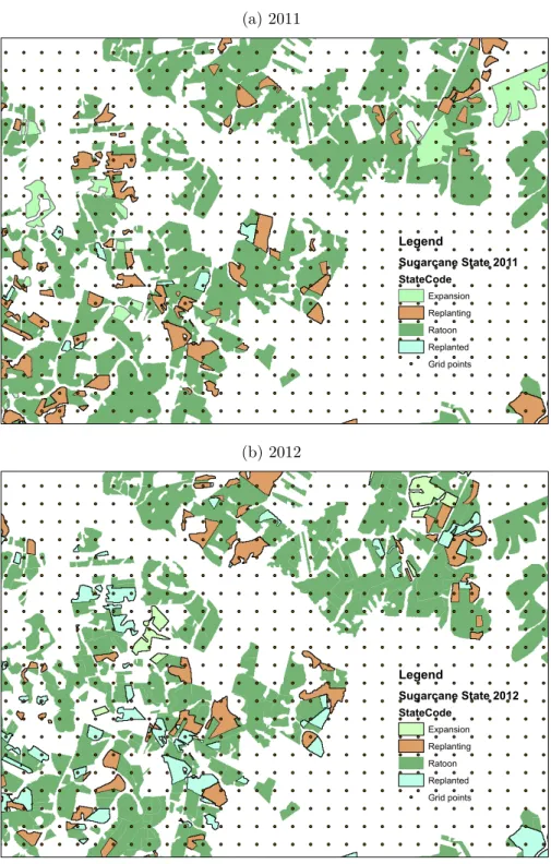
Figure 2 shows one specific producing area in detail. The shapes in the figures are sugarcane producing fields. They are colored according to the classification given by the CANASAT project. “Ratoon” refers to sugarcane that has not been replanted in the pre-vious cycle; “replanted” refers to fields that were replanting in the prepre-vious cycle; while “replanting” refers to fields being replanted in the current cycle; finally, “expansion” refers to new fields that are for the first time available for harvest.

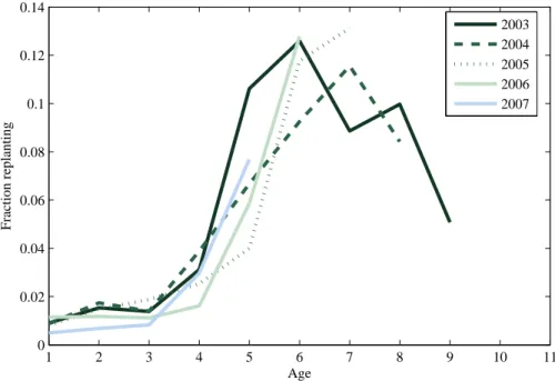
Land use decisions are tracked for each grid point over time, creating a panel data of sugarcane land use. Figure 3 shows the fraction of fields replanted by field age for various cohorts. The observed mode of replanting is 6 years, which is consistent with industry description of replanting decisions. Replanting at higher ages is also frequent, even though not the recommended practice by agronomists, who recommend replanting be done not after 5 years. This suggests that achieving higher yields would be possible by increasing the replanting rate.

There is an important caveat about the remote sensing information. Keeping track of the replanting decision requires the observation of more subtle variation in the satellite imagery at specific moments in the year than what is required to simply identify a sugarcane field. Depending on the variety used or on the time of the year replanting is done,8 _{the imaging} process may fail to identify the replanting activity. So it is expected that some fields are erroneously coded as not replanting in a given year, when in fact they were replanted. I deal with this issue explicitly when estimating the model.

4.2

Distances and transportation cost

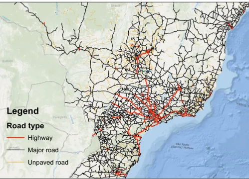
I use data on the Brazilian road network from the Ministry of Transportation and the average speed on each road type to adjust for road quality. This allows me to measure road distance

8_{In general mills have excess capacity in non-harvest months, so it is not uncommon for}

between two points taking into account the quality of the road network on the optimal path. More details about the construction of this transportation network are provided in Appendix A.2. Figure 4 shows the map of the available road network in the Center South Region. The network is more dense close to the shore and becomes more sparse as we move further into the hinterland.

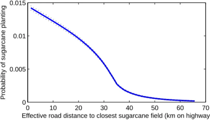
The first use of this distance measure is to compute, for each year, the distance of every grid point to the current closest sugarcane field (variable dit). Figure 5 shows the relation

between proximity of existing sugarcane fields and the decision to plant sugarcane for the first time. There is a sharp decline in the probability of sugarcane adoption as we move away from existing fields. This suggests a sluggish pattern of sugarcane expansion, as new sugarcane is usually planted very close to existing fields.

I further use the transportation network to compute transportation costs from every point in the grid to the closest maritime port. I complement the transportation network with actual freight quotes to estimate a simple model of transportation costs. I use freight quotes from SISFRECA (2008), which surveyed transportation quotes for moving sugar from 177 origins to one of three destination ports (Paranaguá, Guarujá and Santos).

The transportation cost model assumes a linear pricing schedule for freight rates. There is a fixed rate F C independent of distance traveled and a per kilometer on highway rate V C. Equation 7 describes the total cost of moving commodities from location i to j.

TCij = F C + V C × EffectiveDistanceij + νij, (7)

where EffectiveDistance_ij is on highway equivalent distance between i and j, and νij is

an error term, assumed exogenous. I compute effective distances for each one of the 177 origin-destination pairs using the constructed transportation network and estimate fixed and variable costs in equation (7). Results are shown in Table 1. I estimate a US$18.24 fixed cost and US$0.039 per kilometer on highway variable cost of moving one tonne of sugar.

maritime port. I consider as available ports all ports, that according to the Ministry of Transportation had reported any trading of sugar or ethanol. I use the estimated model and these effective distances to calculate transportation costs for all grid points (variable

tci). Figure 5 shows that grid points with a lower transportation cost to ports had a higher

conditional probability of planting sugarcane.

4.3

Other field characteristics

I use as sugarcane potential yield, ys

i, the agro-ecological potential yield from FAO/IIASA

(2011). FAO provides high-resolution potential yield for a variety of crops for all regions of the globe. Those potential yield measures take into account a wide range of soil and climate characteristics relevant for agricultural productivity. Figure 5 shows the relation between the measure I use of sugarcane potential yields and sugarcane planting. The conditional probability of sugarcane planting increases sharply for at values of potential yields above 7 ton. DW/ha. The variation in potential yields shifts the agricultural profitability in a similarly to permanent price changes. Therefore, this variation will be valuable to estimate the effects of counterfactual permanent price increases. The noticeable decline in planting at very high yields highlights the importance of accounting for alternative land uses, as potential yields for different crops are correlated.

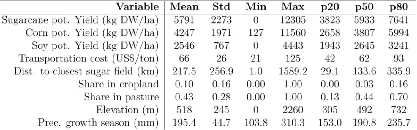
The dataset used to estimate the model is complemented with extensive information on land characteristics described in Table 2, such as climate variables and elevation. Informa-tion on previous land economic use (variable hi) is from Ramankutty et al. (2010a) and

Ramankutty et al. (2010b), which classified all land in the globe into cropland and pasture. I note the higher average share of pasture (0.43) in our sample area, which has led many9 _to believe that most of new sugarcane fields would replace old pasture.

4.4

Prices

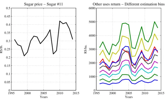
As argued in Section 2, I consider one single market for sugarcane final products, that includes both sugar and sugarcane ethanol. I use the NYSE price of sugar as the reference final product price. This was was pointed as the relevant reference price for decision making in industry discussions. The converted price series to Brazilian Reais (R$) is shown in Figure 6. The observed up and downward swings in prices provide variation in agricultural profitability that is helpful for the estimation of the model.

Equation 8 defines the return index for land not planting sugarcane. It is a weighted sum of the return of alternative agricultural commodities, with the weights given by the relative importance of those other crops in the field region:

rit =

X

c∈{corn,soy}

pc_tαc_iy_ic, (8)

where pc_t denotes the price of crop c, αc_i is a measure of the share10 of crop c in the region of field i and y_icis the FAO/IIASA potential yield of crop c in field i. Corn and soy correspond to more than half the cropland not in sugarcane in this region. Note that this is a contin-uous state variable since potential yield measures are contincontin-uous. For practical estimation purposes, I bin the grid points based on cross section categories for rit based on the expected

returns for the alternative crops. Figure 6 plots the index rit over time for the different

estimation bins.

5

Estimation

I estimate the parameters in the model by Maximum Likelihood. The goal of the estimation is to recover the vector of parameters θ from observed states {wit, ait}it and decisions {˜qit}it,

10_{Shares of land used for corn and soy are obtained from the 2006 Agricultural Census and}

refer to Meso Administrative Regions in the Brazilian Institute of Geography and Statistics (IBGE) classification.

where I make the distinction between observed decisions ˜qit and actual decisions qit. This

distinction will be more clear shortly. Assumption 2 implies that the evolution of the ex-ogenous state does not depend on current endex-ogenous states or field management decisions. Therefore, we can write the conditional log-likelihood criterion function as

L(θ; {˜qit, wit, ait}it) = X t X i log f (wit|wit−1; θ) + X i log (Pr(˜qi|wi, ai; θ)) , (9)

where I omit the subscript t to denote the whole vector of decisions and states.

Note that the only exogenous state variables in wit that change over time are (pst, rit).

For estimation purposes, I assume (ps

t, rit) follow an AR(1) process:

    ps t rit     =     ks kri     +     λs 0 0 λri         ps t−1 rit−1     + ηt, (10) where ηt∼ N     0, σ 2 s 0 0 σ2 ri     .

The exogeneity of the wittransition implies that we can estimate k, λ and σ in a separate

first step. I then treat those parameters as known when maximizing the second term in the likelihood function (equation 9) with respect to the payoff parameters. This procedure is discussed in more detail now.

The remote sensing exercise may fail to capture replanting if it happens in an unusual period of the year or depending on the sugarcane varieties used. This creates classification error, as some fields will be classified as not replanting, ˜q = keep, when indeed replanting

happened. If a field is not coded as replanting, I cannot be sure this actually reflects classi-fication error or just a long sugarcane cycle. If left untreated, this issue could bias upwards our estimated cost of field replanting. I treat classification error as a field specific unobserved state ui ∈ {1, 2}. If ui = 1, there is no classification error on field i remote sensing

replanting decisions on field i are not observed, that is, ˜qit = keep even when qit = replant.

Note there is only classification error for replanting, the decision to plant sugarcane is not subject to observational problems. I assume Pr(ui = 1) = µ for all i. We can write the

conditional probability of observed choices as:

Pr (˜qi|wi, ai; θ) = µ Y t Pr (˜qit|wit, ait, ui = 1; θ) + (1 − µ) Y t Pr (˜qit|wit, ait, ui = 2; θ) . (11)

The choice probability Pr (·|wit, ait, ui = 1; θ) is exactly the model’s CCP (equation 6)

for all ait ∈ {0, 1, . . . , ¯a}, since in this case there is no classification error. However,

Pr (·|wit, ait, ui = 2; θ) is only equal to the model CCP when ait = 0, that is, for fields not

planting sugarcane. For ait> 0 and ui = 2, only ˜qit = keep is coded, so Pr (keep|wit, ait, ui = 2; θ) =

1.

The model’s CCP depends in principal on the full solution of the dynamic discrete choice problem since vθ(ait, wit, q) depends on the continuation value E [Vθ(ait+1(ait, qit), wit+1, εit+1)|wit].

Solving the dynamic discrete choice problem by value function contraction at every different likelihood evaluation is computationally demanding. I use the Nested Pseudo Likelihood (NPL) method proposed by Aguirregabiria and Mira (2002) to circumvent this problem. Instead of solving the dynamic problem at every different likelihood evaluation, this method uses a single contraction in the space of CCPs. I embed the NPL algorithm with an Expec-tation Maximization (EM) step to account for classification error following Arcidiacono and Miller (2011).

Standard errors for payoff parameters are computed by bootstrap. The bootstrap proce-dure follows the estimation steps. For each bootstrap repetition, I re-estimate transportation costs to ports using a bootstrap sample of freight quotes. Additionally, I re-estimate the tran-sition process (equation 10) using a parametric bootstrap sample of prices. I then re-estimate the full model with a block bootstrap sample of observations. I discuss estimation details in

Appendix B.

5.1

Estimation results

Table 3 shows the estimates for the processes in equation (10). In the first column we present the bin number for each category of rit. The second and third column show the values of the

weighted yields for corn and soy that define each bin. The other columns show estimates and standard errors for the auto-regressive processes. The estimated transition for pts is shown

at the bottom of the table.

There is no sign of violation in the stationarity assumption in any of the processes, even though standard errors are relatively high. There is a trade-off here between using a longer price series in dollars and a shorter series measured in the Brazilian currency, Real (R$), which was only adopted in 1994. I opt for the second, since this seems to be the appropriate reference price, especially in terms of volatility, for decision makers in this market. Moreover, it is not clear that using very old price information adds much to the analysis given changes in market dynamics in recent decades.11 _{The cost of relying on} relatively recent price information is a short time series. Imprecision in the estimation of those processes will be taken into account when we compute standard errors for the dynamic model estimates.

In the model section, the functional form for the cost of sugarcane planting, ΨE(hi, dit; θ),

was left unspecified. In estimation, I use the following empirical specification for this cost:

ΨE(hi, dit; θ) =

X

l={crop,pasture,other}

ψ_hl1{hi = l} + ψd1dit1{dit≤ 40} + ψ2d1{dit > 40}. (12)

11_{For instance, it was common in the past to observe price spikes whenever there were}

stock-outs (Deaton and Laroque, 1992). Those type of stock-outs were not seen in recent decades.

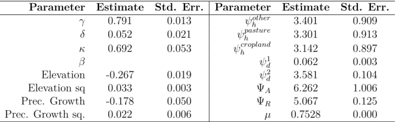
Table 4 shows the results from the NPL estimation of the payoff functions (equations 2 and 3) and fixed cost parameters. I find a steep rate of yield decay from sugarcane field age of 0.79, which represents an expected yield half life of approximately 3 seasons. Current available information about yield decay for sugarcane is restricted to surveys for specific regions and years. For instance, Crago et al. (2010) finds a less steep yearly decay rate of 0.86 using survey information restricted to the state of São Paulo in 2007. Their assessment, however, only considers the first 5 harvests. Taking into account that replanting takes one season, a decay rate of 0.79 implies that the replanting age that maximizes average expected yields is 3 years. This is in line with recommended agronomic practices, that suggest 3 years as a minimum age for field replanting. However, given the positive fixed cost of replanting, we rarely see such short sugarcane cycles, as observed in Figure 3.

I estimate a lower conversion cost for land previously being used for crops in comparison to land used for pasture or in other use. Consistent with descriptive evidence discussed before, I find a high penalty in the cost of planting sugarcane from the distance to existing sugarcane fields. This penalty implies that the increase in fixed cost associated with moving away from existing sugarcane fields by only 10 km is approximately 40% of the revenue associated with the first sugarcane cut of an average sugarcane field.

6

Counterfactuals

6.1

Counterfactual elasticities

I use the estimated model parameters to compute a supply elasticity from permanent price changes, which is then decomposed in yield and acreage components. There is a challenge in evaluating responses to permanent price changes in this setting. The importance of proximity to other fields for sugarcane adoption creates path dependence in the expansion pattern of new sugarcane fields. Therefore, initial conditions matter to determine the system evolution. Motivated by this, I compute price elasticities in the following way. Starting from the current

state of all fields in the sample at the last year available (2012), I simulate a 5% permanent price increase in the sugar price. I compare the evolution of this system under the new price regime to the baseline case of no price increase to calculate acreage and yield effects attributable to the price increase. The acreage effect refers to the additional number of grid points in sugarcane in the counterfactual simulation in comparison to the baseline case. The yield effect refers to the change in average output per field that follows the price increase.

Long-run supply side elasticities are reported in Table 5. I find an acreage elasticity ξL of 3.94, which is 12 times higher than the estimated yield elasticity ξY_{, for which I find a}

value of 0.32. This acreage to yield elasticity ratio means that, at the margin, only 7.66% of the increase in long-run supply comes from higher yields, the other 92.34% comes from acreage expansion. The combined effect of acreage and yield elasticities translates into a supply elasticity of 4.18.

The small contribution of yields at the margin does not mean the yield effect generated by a more intensive pattern of replanting studied here is small. In fact, the yield elasticity

ξY is actually in the ball park of estimates for different crops.12 _{The novelty here is actually} the very high acreage elasticity. In comparison, Miao et al. (2015) find a corn yield elasticity of 0.23 and an acreage elasticity of 0.45 using US data. In the context of global agriculture supply, Roberts and Schlenker (2013) find a much lower acreage elasticity of 0.1. Using a forward looking model of land use in the US, Scott (2013a) finds a higher acreage elasticity of 0.3, still much lower than the value found here.

Three effects combine to determine the high acreage elasticity for sugarcane in Brazil I document here in comparison to other studies of land use. First, I use a dynamic model to

12_{There is little consensus however on the magnitude of yield elasticities. Scott (2013b)}

uses indirect evidence from fertilizer use and finds that yield elasticities for corn are unlikely to be larger than 0.04. Miao et al. (2015) presents a good summary of other results in the literature, which range from not statistically significant to 0.61, depending on the crop studied and methodological approach.

derive the long-run elasticity, while some of the previous studies have only focused on short run acreage responses (Roberts and Schlenker (2013), Miao et al. (2015)). In this sense my results go in the same direction as Scott (2013a), who finds higher acreage price elasticity once forward looking behavior is taken into account. Second, as in Miao et al. (2015), this paper focuses on a single crop, so there is the possibility of cross crop substitution. This is in contrast to Roberts and Schlenker (2013) and Scott (2013a), which aggregate agricultural markets and consider responses to an aggregate price index. Third, Brazil has a very active agricultural frontier, with large extents of undeveloped land, still shy from realizing its agricultural potential.

In this sense, my results highlight the pitfalls of extrapolating cross-country measures of acreage elasticity to study land use. Using the acreage elasticity estimated by Scott (2013a) for the US in our analysis would imply that 45% new ethanol at the margin would come from the intensive margin. This would imply less expansion in farmland as we move along the supply curve and thus a downward bias in expected deforestation.

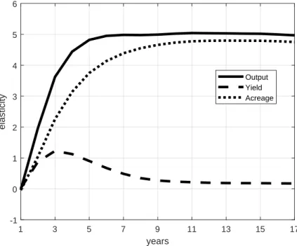
Figure 7 shows the evolution of output, acreage and yield elasticities in the first years after the permanent price shock. The permanent price change encourages expansion of sugarcane to new areas. The expansion of sugarcane in comparison to the baseline translates into acreage elasticities reported in Figure 7. Those new sugarcane fields have higher expected yields than the average pool of sugarcane fields, so yield elasticity jumps in the first periods. As those new areas age, the yield elasticity converges to its long-run value, which reflects the more intensive pattern of replanting that follows the permanent price increase. The output elasticity combines the effects of yield and acreage elasticities. This explains why the output elasticity is steeper than acreage elasticity in the first periods and the faster speed of convergence to the long-run, in comparison to acreage. Although, the focus of this paper is not the short-run dynamics of this market, it is still interesting to note how the yield and acreage effects studied here combine in the short-run to generate a faster response of output in comparison to acreage.

6.2

Deforestation and carbon “payback” times

The acreage and yield elasticities reported in Table 5 suggest that almost all new sugarcane produced following demand shifts in ethanol would come from new growing areas (extensive margin) and not from more intensive replanting cycles (intensive margin). This is a reason for environmental concern, since land use change accounts for a significant part of world greenhouse gas emissions.13

In fact, most of the controversy regarding the use of ethanol biofuels comes from the trade-off between the one-shot emission from land conversion and the carbon emissions avoided over time by replacing fossil fuels by a renewable source. A standard measure used to describe this trade-off is the carbon payback time, i.e., the time it takes for the benefits from replacing fossil fuels to compensate the land use change emissions.14 For the case of sugarcane ethanol there is little consensus for carbon payback times. This could vary from 5 to more than 100 years, depending on assumptions regarding the type of land cover substituted by sugarcane (Searchinger et al. (2008), Elshout et al. (2015), Gibbs et al. (2008), Fargione et al. (2008)). If the land converted to sugarcane fields comes from areas of natural cover with high carbon storage, e.g., tropical forests, the carbon payback time is going to be high. In turn, if land with a lower carbon retention is converted, e.g., cropland and pasture, the carbon payback time will be smaller.

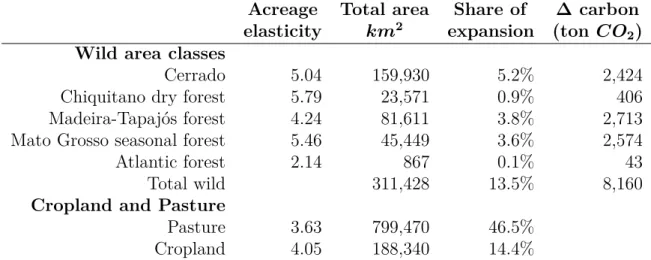
I use the estimated model to predict the direct effect of sugarcane expansion in different natural ecosystems from permanent price shifts. Table 6 shows a decomposition of acreage changes on different areas of natural cover and on existing cropland and pasture. The first column reports acreage elasticities of sugarcane for the different land covers. The third

13_{According to IPCC (2014), deforestation accounted for 12% of global anthropogenic CO}

2 emissions.

14_{It is important to note that the carbon payback time is not a sufficient measure for a}

normative analysis. However, several studies of biofuels have used this measure, which allows comparisons across studies.

column shows the share of each type of land converted to sugarcane at the margin in the long-run.

The last column in Table 6 reports expected carbon emissions from each natural cover for an 1 km2 _{sugarcane expansion at the margin.}15 _{Even though the Cerrado region is the} one with the highest predicted decrease in natural cover, emissions of the same magnitude are predicted to come from land conversion of the two ecosystems connected to the Amazon rainforest, the Madeira-Tapajós and Mato Grosso seasonal forests. This reflects the higher carbon density in the Madeira-Tapajós and Mato Grosso forests compared to the Cerrado.

A few caveats are in order. First, the model does not distinguish between areas of natural cover and cleared areas not in cropland or pasture. The predicted expansion reported ignores specific fixed costs of land clearing and environmental regulation that could restrict deforestation. In this sense, my measure of deforestation and carbon emissions are worse case scenarios. However, this is not the case for pasture and cropland conversion to sugarcane, as I allow the fixed cost of sugarcane planting to vary depending on these two types of land use. Moreover, my analysis focuses only on the Center-South region of Brazil, which includes only the Southern fringe of the Amazon rainforest, which is likely to be the most affected by the expansion of farmland. For a specific treatment of the demand for deforestation in the entire Brazilian Amazon rainforest, see Souza-Rodrigues (forthcoming).

The carbon emission reported in Table 6 represents only direct deforestation by sugarcane expansion, which could be aggravated by indirect land use substitution. Note that, out of sugarcane expansion at the margin, 60% is expected to come from areas already in some economic use, either in cropland or pasture. The substitution of these areas for sugarcane will arguably decrease the supply of agricultural products and may cause additional deforestation as prices of those products increase. The amount of additional land use change from this

15_{The assessment of carbon emissions comes from IPPC guidelines for the evaluation of}

emissions from land use change (IPCC, 2006); I leave the details of this computation to Appendix C.

indirect channel will crucially depend on the relative importance of demand and supply elasticities for the agricultural commodities displaced. Estimates in the literature for those elasticities (Roberts and Schlenker, 2013) suggest that 2_{/3 of productive areas displaced by} sugarcane could move further into the agriculture frontier, causing additional deforestation.16 In order to put those values of carbon emissions from land use change in perspective, one should consider the carbon that could be saved over time by replacing fossil fuels by sugarcane ethanol. Not taking into account emissions from land use change, sugarcane ethanol is supposed to avoid 84% of carbon emissions from gasoline, or 1, 979 kg CO2 equivalent per

m3 _{(Macedo et al., 2008). This measure already includes the use of fossil fuels and energy} in the several stages of the production of sugarcane ethanol, including farm operations and the manufacturing of ethanol from sugarcane.

I balance the carbon that is expected to be released by direct and indirect deforesta-tion with the carbon saved by fossil fuel substitudeforesta-tion to compute long-run carbon payback times for sugarcane ethanol. Table 7 shows payback times for different assumptions on the magnitude of the indirect land use change (ILUC). I find 4.6 years payback for sugarcane ethanol, considering only direct deforestation effects. Assuming that 2_{/3 of the expansion} over other cropland and pasture converts into further deforestation, I find a higher payback time of 18.2 years. This time could be increased to almost 25 years in the extreme case in which all cropland and pasture converted to sugarcane ends up expanding into forests. This extreme case would only be realized if the ratio between supply and demand elasticities for the commodities displaced by sugarcane is infinite. This extreme case provides an upper bound for the sugarcane ethanol carbon payback time.

The sensitivity of the carbon payback times to indirect land use change computed here

16_{There is little evidence however on the direct relationship between the expansion of}

sugarcane and deforestation in the Amazon region through indirect land use change (de Sá et al., 2013). Nevertheless, this indirect land use change could happen in other parts of the world if the agricultural commodities affected are traded internationally.

merits extra attention and should be a topic of future research. The deforestation from indirect land use change might be pivotal in a welfare assessment of sugarcane ethanol policies. However, the carbon payback times in any scenario are dwarfed compared to US corn ethanol, which pays back in 167 years (Searchinger et al., 2008). This difference is primarily due to a lower carbon efficiency in corn ethanol production in comparision to sugarcane.

6.3

Ethanol mandates

In this section I use the estimated model to discuss the effects of biofuels policies. There is a range of ethanol policies in the world today. Here I focus on the most common ones: those that shift the demand for ethanol by establishing ethanol blending standards in trans-portation fuel. Brazil, like many countries, establishes a fixed proportion of ethanol blend in gasoline. Although some States in the U.S. have similar rules, the Federal policy establishes only an aggregate volume of ethanol to be blended to gasoline every year. For simplicity, I study here the effects of shifts in the demand curve for ethanol that would be implied by those mandates.

There are some important caveats in the analysis that follows. First, the results so far concern only the supply side of sugarcane ethanol. Evaluating the effects of demand shifts in this market will require some knowledge of the demand side. I do not estimate a demand elasticity in this paper; instead, I rely on existing results from the literature and assess the robustness of my findings. Second, I estimate the long-run price increase that follows the demand shift using a static equilibrium model. This is in contrast to my measure of supply elasticity that was derived using a dynamic model. I believe that a static equilibrium framework provides a parsimonious environment to study the long-run effects of ethanol mandates.

As an illustrative policy experiment, I consider the effect of the 2007 EISA,17 _which

establishes increasing mandates for ethanol in a nested system. EISA sets an increasing total mandate for renewable fuels from 18 billion gallons in 2014 to 36 billion gallons in 2022 but is subject to EPA rulemakings, which can allow for lower standards each year.18 _Table 8 describes the mandated volumes of biofuels for selected years. The first column shows the total volume of biofuels to be blended. The second column defines the amount that must be met with advanced biofuels and the third column, the amount of the advanced biofuels mandate that must be met by cellulosic biofuels.

In order to meet the mandate, biofuels must achieve at least a 20% reduction in life cycle greenhouse19 _{emissions in comparison with gasoline and diesel. Under the non-advanced} biofuel category falls almost all corn based ethanol produced in the US. Advanced biofuels must achieve at least a 50% reduction in greenhouse gas emissions in comparison with fossil fuels. Finally, cellulosic biofuels refer to biofuels derived from any cellulose that achieve a 60% gain in terms of greenhouse gas emissions. There was not much interest from the private sector in cellulosic ethanol mainly because the necessary conversion technology is still too costly for large scale application (Bracmort, 2012). As consequence, EPA has been continuously using its statutory authority to the waive cellulosic biofuels mandate on the

18_{The EPA has the stutory authority to waive the biofuels mandate in the cases of}

“in-sufficient supply” or “economic harm.” For example, for 2019 the EPA set the final volume of ethanol in the standard to 19.2 billion gallons, below the volume predicted in EISA. It is likely that EPA will continue to set lower stadard volumes of ethanol in the following years.

19_{According to EISA 2007 sec. 201, “‘lifecycle greenhouse gas emissions’ means the}

aggre-gate quantity of greenhouse gas emissions (including direct emissions and significant indirect emissions such as significant emissions from land use changes), as determined by the Admin-istrator, related to the full fuel lifecycle, including all stages of fuel and feedstock production and distribution, from feedstock generation or extraction through the distribution and de-livery and use of the finished fuel to the ultimate consumer, where the mass values for all greenhouse gases are adjusted to account for their relative global warming potential.”

basis of “insufficient supply.”

Brazilian sugarcane ethanol is classified by the EPA as an advanced biofuel. In fact, it is the sole large scale source of Advanced Biofuels in the EPA classification. I consider a counterfactual shift in the world demand of sugarcane ethanol of 5 billion gallons, which is the volume in the advanced biofuel category that needn’t be met by cellulosic biofuels (21 − 16 = 5, in 2022, Table 8). This value is not far from the final advanced biofuel mandate set for 2019 by the EPA of 4.9 billion gallons.

Table 9 shows aggregate effects on prices, acreage expansion and yields in Brazil of a 5 billion gallons mandate of sugarcane ethanol. I use a baseline demand elasticity of −0.2 from Elobeid and Tokgoz (2008).20 _{Policy effects are not sensitive to demand elasticities in the} inelastic range. The low price responses and comparatively high acreage responses are driven primarily by the high acreage to yields elasticity ratio I find. This analysis suggests that a 5 billion gallon mandate, which is equivalent to about 3% of US gasoline consumption, could imply about 4,500 sq. kilometers in direct deforestation. Following the previous analysis of indirect deforestation, this could be magnified to 15,900 sq. kilometers if indirect effects are considered considering the baseline 66% indirect land use change effect.

7

Conclusion

This paper studies the economics of land use for the sugarcane ethanol production to quantify the environmental effects of biofuel policies. The expansion in ethanol production may endanger tropical forests, which could offset the carbon savings accrued over time by the replacement of fossil fuels. I use a dynamic model of land use that encompasses both adoption of sugarcane and replanting decisions, which is crucial to disentangle acreage and yield responses to policy changes.

20_{Roberts and Schlenker (2013) find a comparable values of demand elasticities for}

I find a high acreage-price elasticity, which implies much higher acreage to yield elasticity ratios than found in previous studies. The results suggest that ad-hoc assumptions on the pattern of land expansion can severely bias the evaluation of the merits of sugarcane ethanol as a greener replacement for fossil fuels. The most detrimental environmental effects from biofuels demand shifts come from land use change associated with an expansion of biofuels crops. If the acreage to yield elasticity ratio is low, there is scope for yields to absorb the increase in demand. However, if the acreage elasticity is higher than the yield elasticity, the increase in ethanol supply comes primarily from new producing areas.

In the case of Brazilian sugarcane ethanol, I find that the extensive margin (acreage) dominates the intensive margin (yield). This results in large acreage expansion following an increase in feedstock demand and a comparatively small increase in yields. I use the high-resolution nature of the dataset and the estimated model to predict the direct effects on natural land cover and associated carbon emissions. I discuss how indirect deforestation caused by crop and pasture substitution could aggravate land use change emissions. I find lower carbon payback times for sugarcane ethanol compared to US corn ethanol, but these are somewhat sensitive to the importance of indirect land use change, which points in the direction of important future research.

References

Victor Aguirregabiria and Pedro Mira. Swapping the nested fixed point algorithm: A class of estimators for discrete Markov decision models. Econometrica, 70(4):1519–1543, 2002.

Victor Aguirregabiria and Pedro Mira. Dynamic discrete choice structural models: A survey.

Journal of Econometrics, 156(1):38–67, 2010.

Treb Allen and Costas Arkolakis. Trade and the topography of the spatial economy. The

Soren T Anderson, Ryan Kellogg, and Stephen W Salant. Hotelling under pressure. NBER

Working Paper, (20280), 2014.

Peter Arcidiacono and Robert A Miller. Conditional choice probability estimation of dynamic discrete choice models with unobserved heterogeneity. Econometrica, 79(6):1823–1867, 2011.

Steven Berry. Biofuels policy and the empirical inputs to GTAP models. Discussion Paper, 2011.

Kelsi Bracmort. Meeting the renewable fuel standard (RFS) mandate for cellulosic biofuels: Questions and answers. CRS Report for Congress, (R41106), 2012.

Christine L Crago, Madhu Khanna, Jason Barton, Eduardo Giuliani, and Weber Amaral. Competitiveness of Brazilian sugarcane ethanol compared to US corn ethanol. Energy

Policy, 38(11):7404–7415, 2010.

Harry De Gorter, Dusan Drabik, Erika Kliauga, and Govinda R Timilsina. An economic model of Brazil’s ethanol-sugar markets and impacts of fuel policies. World Bank Policy

Research Working Paper, (6524), 2013.

Saraly Andrade de Sá, Charles Palmer, and Salvatore Di Falco. Dynamics of indirect land-use change: empirical evidence from Brazil. Journal of Environmental Economics and

Management, 65(3):377–393, 2013.

Angus Deaton and Guy Laroque. On the behavior of commodity prices. The Review of

Economic Studies, 59(1):1–23, 1992.

Amani Elobeid and Simla Tokgoz. Removing distortions in the US ethanol market: What does it imply for the United States and Brazil? American Journal of Agricultural

PMF Elshout, R van Zelm, J Balkovic, M Obersteiner, E Schmid, R Skalsky, M van der Velde, and MAJ Huijbregts. Greenhouse-gas payback times for crop-based biofuels. Nature

Climate Change, 2015.

EPA. Renewable Fuel Standard Program (RFS2) Regulatory Impact Analysis. 2010.

FAO/IIASA. Global Agro-ecological Zones (GAEZ v3.0). FAO and IIASA, Rome, Italy and Laxenburg, Austria, 2011.

Joseph Fargione, Jason Hill, David Tilman, Stephen Polasky, and Peter Hawthorne. Land clearing and the biofuel carbon debt. Science, 319(5867):1235–1238, 2008.

Holly K Gibbs, Matt Johnston, Jonathan A Foley, Tracey Holloway, Chad Monfreda, Navin Ramankutty, and David Zaks. Carbon payback times for crop-based biofuel expansion in the tropics: The effects of changing yield and technology. Environmental Research Letters, 3(3):034001, 2008.

R.J. Hijmans, S.E. Cameron, J.L. Parra, P.G. Jones, and A. Jarvis. Very high resolution interpolated climate surfaces for global land areas. International Journal of Climatology, 25:1965–1978, 2005.

V Joseph Hotz and Robert A Miller. Conditional choice probabilities and the estimation of dynamic models. The Review of Economic Studies, 60(3):497–529, 1993.

IPCC. 2006 IPCC Guidelines for National Greenhouse Gas Inventories, volume 4. IPCC, Hayama, Japan, 2006.

IPCC. Climate Change 2014: Mitigation of Climate Change. Contribution of Working Group

III to the Fifth Assessment Report of the Intergovernmental Panel on Climate Change.

Cambridge University Press, Cambridge, UK, 2014.

Ryan Kellogg. The effect of uncertainty on investment: Evidence from Texas oil drilling.

Christine Lasco and Madhu Khanna. US-Brazil trade in biofuels: Determinants, constraints, and implications for trade policy. In Handbook of Bioenergy Economics and Policy, pages 251–266. Springer, 2010.

Isaias C Macedo, Joaquim EA Seabra, and João EAR Silva. Green house gases emissions in the production and use of ethanol from sugarcane in Brazil: The 2005/2006 averages and a prediction for 2020. Biomass and bioenergy, 32(7):582–595, 2008.

Ruiqing Miao, Madhu Khanna, and Haixiao Huang. Responsiveness of crop yield and acreage to prices and climate. American Journal of Agricultural Economics, 2015.

Sriniketh Nagavarapu. Implications of unleashing Brazilian ethanol: trading off renewable fuel for how much forest and savanna land. Working Paper, 2010.

N. Ramankutty, A.T. Evan, C. Monfreda, and J.A. Foley. Global Agricultural Lands: Croplands, 2000. Data distributed by the Socioeconomic Data and Applications

Cen-ter (SEDAC): http://sedac.ciesin.columbia.edu/es/aglands.html. (Accessed 09/19/2014)., 2010a.

N. Ramankutty, A.T. Evan, C. Monfreda, and J.A. Foley. Global Agricultural Lands: Pasture,

2000. Data distributed by the Socioeconomic Data and Applications Center (SEDAC):

http://sedac.ciesin.columbia.edu/es/aglands.html. (Accessed 09/19/2014)., 2010b.

Michael J. Roberts and Wolfram Schlenker. Identifying supply and demand elasticities of agricultural commodities: Implications for the US ethanol mandate. American Economic

Review, 103(6):2265–2295, 2013.

B. F. T. Rudorff, D. A. Aguiar, W. F. Silva, L. M. Sugawara, M. Adami, and M. A. Moreira. Studies on the rapid expansion of sugarcane for ethanol production in São Paulo State (Brazil) using landsat data. Remote sensing, 2(4):1057–1076, 2010.

John Rust. Optimal replacement of GMC bus engines: An empirical model of Harold Zurcher.

Econometrica, 55(5):999–1033, 1987.

Paul T. Scott. Dynamic discrete choice estimation of agricultural land use. Working Paper, 2013a.

Paul T. Scott. Indirect estimation of yield-price elasticities. Working Paper, 2013b.

Timothy Searchinger, Ralph Heimlich, Richard A Houghton, Fengxia Dong, Amani Elobeid, Jacinto Fabiosa, Simla Tokgoz, Dermot Hayes, and Tun-Hsiang Yu. Use of US croplands for biofuels increases greenhouse gases through emissions from land-use change. Science, 319(5867):1238–1240, 2008.

SISFRECA. SISFRECA 2008 Yearbook. ESALQ-LOG, Piracicaba, Brazil, 2008.

Eduardo Souza-Rodrigues. Deforestation in the Amazon: A Unified Framework for Estima-tion and Policy Analysis. The Review of Economic Studies, forthcoming.

A. Valente, V. Tani, A. Coelho, M. Pimenta, P. Tome, R. Reibnitz, and R. Queiroz. De-terminacao das velocidades médias de operacao para o ano de 2006. Technical report, 2008.

Appendix

A

Data

A.1

Panel of sugarcane land use

I create a 1km grid of points encompassing all micro-regions in Center South Brazil that had reported sugarcane areas in the remote sensing dataset. I exclude urban areas as well as water bodies, such as lakes and large rivers. Moreover, I exclude grid point in the Pantanal eco-region. There is a strict ban on sugarcane growing in this area. In fact, I found no reports of sugarcane growing in this region. The resulting grid extends through 6 States in Brazil.

The remote sensing maps only inform new fields as well as replanting decisions for existing fields. Therefore I can only track the age of a given sugarcane field if it is a new field in my sample or if it replants.

A.2

Distances and transportation cost

Using existing road information from the Ministry of Transportation, we build a road network that covers the entire region of interest. We classify each road type in terms of average traveling speed of trucks relative to highways (the best road type available). This gives a measure of relative cost of traveling over each point in the map. We consider 1 km on highway to be equivalent to 1.25 km on a major road, 1.66 km on unpaved road and 2.5 km everywhere else. Those values are informed by Valente et al. (2008), which surveys traveling speed of different types of vehicles. As an example, suppose the best route between i and j is 1 km on a dirt road, then we consider that effective distance between i and j to be 1.66

km.