A new approach for RIM: from RIMCop
technology to process design
Ph.D. Dissertation in
Mechanical Engineering by
Nuno Miguel de Oliveira Gomes
SupervisorsJosé Carlos Brito Lopes Ricardo Jorge Nogueira dos Santos
Paulo Jorge da Silva Bártolo
Laboratory of Separation and Reaction Engineering - LSRE Laboratório Associado LSRE/LCM
Departamento de Engenharia Química
Faculdade de Engenharia Universidade do Porto
Acknowledgments
I wish to express my gratitude to all whose contribution was fundamental in completion of this work:
Prof José Carlos Lopes, my advisor, for his guidance, support during this course of the work and giving an opportunity to be part of this Mixing Group;
Dr. Ricardo Santos, my co-advisor, for his guidance, support, patience, time and effort during this course of this work and being a friend;
Prof Paulo Bártolo, my co-advisor, for support and the opportunity to start on research;
Profª Madalena Dias for the review of my work during my work and for support and suggestions;
Prof Artur Mateus, for the guidance and to introduced me on Reaction Injection Moulding;
Prof Alírio Rodrigues, director of LSRE, where part of this work was carried out; Susana Cruz, for her administrative support at LSRE;
Dr Carlos Sá and Dra Daniela Silva, both from CEMUP, for SEM analysis and help; Profª Fátima Barreiros, Prof Pedro Martinho, former directors of Departamento de
Eng Mecânica of Instituto Politécnico de Leiria, where part of the work was carried out, Prof. Joel Vasco, responsible of Lab. de Tecnologias Mecânicas and Prof Mário Pereira, responsible of Lab de Materiais;
My coworkers in the Lab de Tecnologias Mecânicas, Tiago Nunes, Carlos Mota, Dinarte Abreu, Eduardo Farinha, and specially to my friend Carlos Dias, for the all support and discussion;
My coworkers in LSRE, Carlos Fonte, Anna Maria Karpsinka, Nuno Gomes, Marina V. Torres, Kateryne Kruppa, Angela Novais and Enis Leblebici, for their help, friendship and specially to Cláudio Fonte for value discussions and patient;
My friends, for weekend breaks in Leiria, Ana Rita, Andreia, André, Pedro, Joana and Hugo Carriço, and for week breaks in Porto, Ashar, Julio and Rui;
Francisco Gomes, for his support in all kinds of machining and ideas; José Gomes for his help and guidance;
Maria Isabel and Sara, for their support and valuable ideas for work and the thesis; Rita, for her love, support and patience;
Finally, to Portuguese Foundation for Science and Technology, for supporting this research work and the result dissemination activities under the grant SFRH/BD/45621/2008;
Abstract
The present work concerns the study of RIMCop technology and Reaction Injection Moulding (RIM) process design. RIMCop is a patented technology to improve the mixing in the RIM process. The process design consisted in the setting of RIMcop machine parameters and of the mould filling. Computational Fluid Dynamics (CFD) tools were used to compare five different commercial types of RIM mixing chambers that were assessed from dimensionless maps of vorticity, pathlines and strain rate. Also an energy balance and the Residence Time Distribution (RTD) were measured. The results showed that the simplest T-jet configurations are more suitable as far as RIM mixing is regarded. A new project for new industrial prototype equipment was introduced.
Experimental study on poluyrethane mixing using a T-jet configuration, showed a dependency of the material properties on the pressure difference at the mixing head, *
P
, and it was also found that the pressure signal oscillates with typical frequencies. Based on these results, an impingement point position model was introduced. RIMCop technology proposes a unitary kinetic energy ratio between jets, KEr 1, for best mixing performance. Experimental results showed that KEr influences theadiabatic temperature rise, and reaction kinetics. Physical and mechanical properties, such as density, deflection temperature, glass temperature, tensile, compressive and flexural properties clearly showed the influence of KEr.
The RIM mould filling process was modeled with CFD using 2D and 3D models and Volume of Fluid model. The obtained results were in good agreement with available literature. This model was used for contracting and expanding flows. Four main phenomena were identified on RIM mould filling: stable front, air entrapment at salient corner, air entrapment and engulfment and air boundary layer; and were studied considering the effect of the gravitational, viscous, inertial and surface forces. From the CFD results were obtained maps with the occurrence of each particular phenomenon as function of some dimensionless numbers, aiming the selection of processing conditions. Also some considerations for calculating the thickness of mould plates, gate location and venting zone dimension were introduced.
Resumo
A presente dissertação dedica-se ao estudo da tecnologia RIMCop e ao projeto do processo de RIM. O RIMCop é uma tecnologia patenteada para melhorar a mistura durante o processo RIM. O projeto do processo consistiu na definição dos parâmetros de funcionamento duma máquina RIM com a tecnologia RIMCop e do enchimento do moulde.
Usando ferramentas de Computação de Fluídos Dinâmicos (CFD), cinco câmaras de mistura comerciais foram comparadas, e analisadas de acordo com os seus mapas adimensionais de vorticidade, linhas de fluxo e taxa de deformação. Também foi feita uma analise do balanço energético, e da distribuição dos tempos de residência. Os resultados mostram que as câmaras de mistura em T, são as mais adequadas para o RIM. Foi introduzido um novo projeto para um equipamento protótipo a nível industrial.
Estudos experimentais na produção de poliuretano, usando uma câmara de mistura em T, mostram a dependência das propriedades do material da diferença de pressão na cabeça de mistura,
D
P
*, bem como a existência de valores típicos de frequência nas oscilações do valor da pressão diferencial. Um modelo para a posição do ponto de impacto foi introduzido com base nos resultados. A tecnologia RIMCop propõe que a razão da energia cinética dos jactos deverá ser igual a um, KEr 1, de modo a melhorar a mistura. Resultados experimentais mostram que KErinfluencia a subida de temperatura adiabática, e a cinética da reação. Propriedades físicas e mecânicas, como a densidade, temperatura de defleção, temperatura vítrea, propriedades de extensão, compressão e flexão, mostram uma clara influência de KEr.
O processo de enchimento de mouldes em RIM foi simulado em 2D e 3D com ferramentas de CFD. Os resultados obtidos estão de acordo com os encontrados na literatura. Este modelo foi aplicado ao estudo do escoamento em contracções e expansões 2D. Quatro principais fenómenos foram identificados, e descritos: frente de escoamento estável, aprisionamento de ar no canto saliente, aprisionamento de ar no seio do escoamento e uma camada-limite de ar; sendo estudados de acordo com as forcas gravitacionais, viscosas, inerciais e de superfície. Os resultados obtidos permitiram a construção de mapas de ocorrência de cada fenómeno, em função de alguns números adimensionais, de modo a ajudar na selecção das condições de processamento. Foram apresentadas, ainda, algumas considerações para o cálculo da espessura das chapas dos mouldes, localização dos pontos de injeção e zonas de ventilação.
Page
1 Introduction ... 2
1.1 Reaction Injection Moulding ... 2
1.2 Relevance and Motivation ... 6
1.3 Thesis Objectives and Layout ... 7
1.4 References ... 8 2 State of Art ... 9 2.1 Mixing Head ... 9 2.1.1 L Mixing Head ...10 2.1.2 T Mixing Head ...13 2.1.3 Geometrical Studies ...20
2.2 Mixing Analysis Method ...23
2.2.1 Mixing and Reaction Studies ...26
2.2.1.1 Product Distribution from Test Reactions ...26
2.2.1.2 Tracer Studies ...27
2.2.1.3 Physical Characteristics of the Final Polymer ...28
2.2.1.4 Adiabatic Temperature Rise ...28
2.3 Numerical Simulation of RIM Process ...29
2.4 Project Rules for RIM’s Moulds ...32
2.5 Conclusions ...40
2.6 References ...42
3 RIMCop technology project ...49
3.1 Introduction ...49
3.2 Mixing-Chamber: Simple or Complex Geometries? ...50
3.2.1 Model ...51
3.2.1.1 Geometric Model ...51
3.2.1.2 Physical Model ...52
3.2.1.3 Boundary Conditions ...53
3.2.1.4 Numerical Method and Discretization ...54
3.2.2 Results ...54
3.2.2.1 Flow Maps ...54
3.2.3 Macroscopic Energy Balance ...80
3.2.4 Residence Time Distribution ...91
3.3 RIMCop System Characterization ...97
3.3.1 RIM Equipment Project ...97
3.3.1.1 Mixing Head ... 100
3.3.1.2 Meetering Pumps ... 104
3.3.1.3 Storage Tanks ... 106
3.3.1.4 Control System ... 111
3.4 RIMCop System Calibration ... 115
3.4.1 CDRsp-IPLeiria Equipment Calibration ... 115
3.4.2 LSRE-FEUP Equipment Calibration ... 116
3.5 Conclusions ... 121
3.6 References ... 122
4 Application of RIMCop Machine ... 127
4.2 Assessment of Mechanical Properties in RIM ... 128 4.2.1 Experimental Setup ... 130 4.2.2 CFD Model ... 133 4.2.3 Results ... 135 4.2.3.1 Mechanical Properties ... 135 4.2.3.2 Spectral Analysis... 136
4.2.3.3 Models for the jets equilibrium ... 143
4.3 Mixing Under Controlled Conditions - RIMCop ... 148
4.3.1 List of Experimental Conditions ... 150
4.3.2 Experimental Setup ... 151
4.3.3 Polymerization Kinetics ... 153
4.3.3.1 Adiabatic Reactor ... 156
4.3.3.2 Results and Discussion ... 160
4.3.4 Physical Characteristics of the Final Polymer ... 164
4.3.4.1 Physical Properties ... 166
4.3.4.2 Mechanical Properties ... 170
4.3.4.3 Morphological Studies ... 182
4.4 Conclusions ... 190
4.5 References ... 191
5 RIM mould design ... 197
5.1 Introduction ... 197
5.2 VOF Model for Reaction Injection Moulding’s Flow Front ... 198
5.2.1 Physical Model ... 200
5.2.2 Results ... 202
5.2.3.1. Filling of symmetric rectangular pipe ... 202
5.2.3.2. Filling of 3D symmetric cavity ... 205
5.3 Filling phenomena and flow maps in thickness variation ... 206
5.3.1 Dimensionless analysis ... 209
5.3.2 Flow phenomena ... 211
5.3.3 Fluid mechanics parameters effects ... 223
5.3.3.1 Effect of gravity – Froude number ... 223
5.3.3.2 Effect of viscous forces – Reynolds number ... 228
5.3.3.3 Surface forces during filling – effect of Weber ... 236
5.3.3.4 Effect of thickness ratio ... 237
5.3.3.5 Velocity Field ... 246
5.3.3.6 Pressure drop ... 249
5.3.4 Flow pattern maps ... 259
5.4 Mould project recommendations ... 262
5.4.1 Mould project ... 262 5.4.2 Filling stage ... 266 5.4.3 . Curing Stage ... 269 5.5 Conclusions ... 272 5.6 References ... 274 6 Final remarks ... 279 6.1 General Conclusions ... 279
6.1.1 RIMCop Technology Project ... 281
6.1.2 Physical Characteristics of Final Polymer ... 283
6.1.2.1 Assessment of RIM ... 283
6.1.2.2 Assessment of RIMcop ... 283
6.1.3 RIM Mould Design ... 284
6.2 Future Work ... 286
6.3 References ... 287
B. Detailed Experimental Procedure ... 292 B.1. Materials ... 292 B.2. Experimental Procedure ... 293
Table of Figures
Page
Figure 1-1 Reaction Injection Moulding scheme (Martinho et al., 2003) ... 2
Figure 1-2 Phenomena associated to the different stages in RIM(Bártolo and Mateus, 2003) ... 4
Figure 1-3 RIM cycle (Martinho et al., 2003) ... 4
Figure 2-1 L Mixing chamber (Schluter, 1976) ...11
Figure 2-2 Several mixing chamber geometries: a) circular b) balloon c) triangular d) rectangular (Tenhagen, 1986) ...11
Figure 2-3 L Mixing head of Schmitz and Krompass (1984) ...12
Figure 2-4 L Mixing head of Schneider (1991) ...12
Figure 2-5 L Mixing head with aftermixing (Schneider, 1984a) ...13
Figure 2-6 Moveable mixing chamber, at a L mixing head (Fiorentini, 1989) ...13
Figure 2-7 T mixing head with two pistons positions: a) injection position b) recirculation position (Keuerleber and Pahl, 1972) ...14
Figure 2-8 RIMCop mixing head (Lopes et al., 2005) ...15
Figure 2-9 Slide valve mixing head: a) mixing position b) recirculation position (Bolde and Schulte, 1994) ...15
Figure 2-10 Rotary valve mixing head, from Cannon: a) mixing position b) recirculation position (Bolde and Schulte, 1994) ...16
Figure 2-11 Wisbay mix –head: a) mixing position b) recirculation position (Wisbey, 1977) ...16
Figure 2-12 Vertically angled mixing head (Macosko and McIntyre, 1984) ...17
Figure 2-13 Recirculation Grooves (Macosko and McIntyre, 1984) ...17
Figure 2-14 Horizontal angled mixing head (Sweeney, 1987) ...18
Figure 2-15 Delivery system with retractable turbulence bar: a) mixing position b) recirculation position (Taubenmann, 1986) ...19
Figure 2-16 Schlueter mixing head in mixing position (Schlueter, 1984)...19
Figure 2-17 Bauer mixing head in mixing position (Bauer, 1985)...20
Figure 2-18 Toda and Hori mixing head in mixing position (Toda and Hori, 1989) ...20
Figure 2-19 Mixing head adopted from Johnson et al. (1996) ...21
Figure 2-20Mixing head Parameters adopted from Bierdel and Piesche (2001) ...22
Figure 2-21 Mixing head used adopted from Teixeira (2000) ...23
Figure 2-22– Spontaneous growth between the two interfaces of mixing phases (Macosko, 1989) ...25
Figure 2-23 Cavity Filling from Michalek and Kowaleski (2003): a) Temperature Profile from PIT b) Temperature Profile from Fluent ...31
Figure 2-24 – Cure degree (Igreja 2007) ...31
Figure 2-25 – Flow around a restriction, where the streamlines represent the flow along time (Müller et al., 1985a) ...33
Figure 2-26 Flow inside an aftermixer (Müller et al., 1985a) ...33
Figure 2-27 Aftermixers: a) peanut b) heart c) dipper and d) harp ...34
Figure 2-28 Direct gate ...35
Figure 2-29 Fan gate ...35
Figure 2-30 IKV version of fan gate ...36
Figure 2-31 Sprue gate with a) frontal inlet b) lateral inlet ...37
Figure 2-32 Dam gate ...37
Figure 2-33 Air or gas venting – at black the venting holes, and at grey the cavity ...38
Figure 2-35 Heating channels: a) thermal balanced b) thermal unbalanced ...39 Figure 2-36 Main dimensions of the heating channels ...39 Figure 2-37 Heating circuits configuration: a) manifold b) single pass ...40 Figure 3-1 Studied Geometries: a) Opposed jets mixing chamber, b) Opposed jets mixing
chamber with restrictions, c) Opposed jets mixing chamber in L configuration, d) Vertically angled jets mixing chamber e) Horizontally angled jets mixing chamber ...52 Figure 3-2 Studied planes from different geometries: a) Opposed jets mixing chamber,
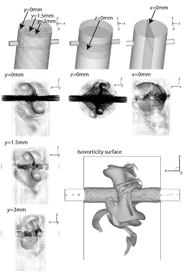
b) Opposed jets mixing chamber with restrictions, c) Opposed jets mixing chamber in L configuration, d) Vertically angled jets mixing chamber e) Horizontally angled jets mixing chamber ...62 Figure 3-3 Non-dimensional Vorticity maps, with pathlines for aRe75, at planes XZ and
XY a) Opposed jets mixing chamber, b) Opposed jets mixing chamber with restrictions, c) Opposed jets mixing chamber in L configuration, d) Vertically angled jets mixing chamber e) Horizontally angled jets mixing chamber ...63 Figure 3-4 Non-dimensional Vorticity maps, with pathlines for aRe75, at plane YZ a)
Opposed jets mixing chamber, b) Opposed jets mixing chamber with restrictions, c) Opposed jets mixing chamber in L configuration, d) Vertically angled jets mixing chamber e) Horizontally angled jets mixing chamber ...64 Figure 3-5 Non-dimensional Vorticity maps, with pathlines for a Re150, at planes XZ
and XY a) Opposed jets mixing chamber, b) Opposed jets mixing chamber with restrictions, c) Opposed jets mixing chamber in L configuration, d) Vertically angled jets mixing chamber e) Horizontally angled jets mixing chamber ...65 Figure 3-6 Non-dimensional Vorticity maps, with pathlines for a Re150, at plane YZ a)
Opposed jets mixing chamber, b) Opposed jets mixing chamber with restrictions, c) Opposed jets mixing chamber in L configuration, d) Vertically angled jets mixing chamber e) Horizontally angled jets mixing chamber ...66 Figure 3-7 Non-dimensional Vorticity maps, with pathlines for a Re300, at planes XZ
and XY a) Opposed jets mixing chamber, b) Opposed jets mixing chamber with restrictions, c) Opposed jets mixing chamber in L configuration, d) Vertically angled jets mixing chamber e) Horizontally angled jets mixing chamber ...67 Figure 3-8 Non-dimensional Vorticity maps, with pathlines for a Re300, at plane YZ a)
Opposed jets mixing chamber, b) Opposed jets mixing chamber with restrictions, c) Opposed jets mixing chamber in L configuration, d) Vertically angled jets mixing chamber e) Horizontally angled jets mixing chamberr ...68 Figure 3-9 Pathlines forRe75, a) Opposed jets mixing chamber, b) Opposed jets mixing
chamber with restrictions, c) Opposed jets mixing chamber in L configuration, d) Vertically angled jets mixing chamber e) Horizontally angled jets mixing chamber ...69 Figure 3-10 Pathlines forRe150, a) Opposed jets mixing chamber, b) Opposed jets
mixing chamber with restrictions, c) Opposed jets mixing chamber in L configuration, d) Vertically angled jets mixing chamber e) Horizontally angled jets mixing chamber ...70 Figure 3-11 Pathlines for Re300, a) Opposed jets mixing chamber, b) Opposed jets
mixing chamber with restrictions, c) Opposed jets mixing chamber in L configuration, d) Vertically angled jets mixing chamber e) Horizontally angled jets mixing chamber ...71 Figure 3-12 Flow imaging: vector maps from dynamic 3D CFD simulation at Re200 for
Opposed jets mixing chamber (Santos et al., 2009) ...72 Figure 3-13 Non-dimensional strain rate field maps, with pathlines for a Re75, at
planes XZ and XY a) Opposed jets mixing chamber, b) Opposed jets mixing chamber with restrictions, c) Opposed jets mixing chamber in L configuration, d) Vertically angled jets mixing chamber e) Horizontally angled jets mixing chamber ...73 Figure 3-14 Non-dimensional strain rate field maps, Re75, at plane YZ a) Opposed jets
mixing chamber in L configuration, d) Vertically angled jets mixing chamber e)
Horizontally angled jets mixing chamber ...74
Figure 3-15 Non-dimensional strain rate field maps, with pathlines for a Re150, at planes XZ and XY a) Opposed jets mixing chamber, b) Opposed jets mixing chamber with restrictions, c) Opposed jets mixing chamber in L configuration, d) Vertically angled jets mixing chamber e) Horizontally angled jets mixing chamber ...75
Figure 3-16 Non-dimensional strain rate field maps, Re150, at plane YZ a) Opposed jets mixing chamber, b) Opposed jets mixing chamber with restrictions, c) Opposed jets mixing chamber in L configuration, d) Vertically angled jets mixing chamber e) Horizontally angled jets mixing chamber ...76
Figure 3-17 Non-dimensional strain rate field maps, with pathlines for a Re300, at planes XZ and XY a) Opposed jets mixing chamber, b) Opposed jets mixing chamber with restrictions, c) Opposed jets mixing chamber in L configuration, d) Vertically angled jets mixing chamber e) Horizontally angled jets mixing chamber ...77
Figure 3-18 Non-dimensional strain rate field maps, Re300, at plane YZ a) Opposed jets mixing chamber, b) Opposed jets mixing chamber with restrictions, c) Opposed jets mixing chamber in L configuration, d) Vertically angled jets mixing chamber e) Horizontally angled jets mixing chamber ...78
Figure 3-19 Isosurface for a non-dimensional vorticity of *2 and a 300 Re , a) Opposed jets mixing chamber, b) Opposed jets mixing chamber with restrictions, c) Opposed jets mixing chamber in L configuration, d) Vertically angled jets mixing chamber e) Horizontally angled jets mixing chamber ...79
Figure 3-20 Geometric Model with a control volume - grey zone - and control surface – dash line ...80
Figure 3-21 Geometric Model of an opposed jets in L, with a control volume - grey zone - and control surface – dashed line. The less sparse dashed line limits the first control volume, and the sparser dashed line limits the second control volume of the mixing chamber. ...88
Figure 3-22 Geometric Model of a vertically angled jets mixing chamber, with a control volume - grey zone - and control surface – dash line. ...89
Figure 3-23 Residence Time Distribution for each geometry and Re the studies a) Opposed jets mixing chamber, b) Opposed jets mixing chamber with restrictions, c) Opposed jets mixing chamber in L configuration, d) Vertically angled jets mixing chamber e) Horizontally angled jets mixing chamber ...96
Figure 3-24 Industrial RIM prototype at CDRsp-IPLeiria, adapted from PLASRIM project ....98
Figure 3-25 Flow scheme of the RIM prototype machine at CDRsp-IPLeiria ...98
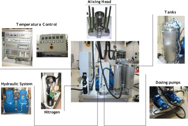
Figure 3-26 Pilot RIMcop® machine at LSRE-FEUP ...99
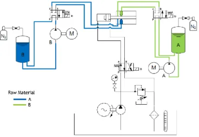
Figure 3-27 Flow scheme of the pilot RIMcop® machine at LSRE-FEUP ...99
Figure 3-28 Patented scheme of RIMCop mixing-chamber (Lopes et al., 2005) ... 101
Figure 3-29 Cad drawing of the Mixing-Head groups: a) Material outlet b) cylinder and cleaning piston c) Mixing-Head Body d) Material Inlet e) exploded view of the Mixing-Head ... 102
Figure 3-30 Cad drawing of the injector. ... 102
Figure 3-31 a) PTS Validyne P55, b) Model Cad of pressure tip, over the different parts . 103 Figure 3-32 RIMcop® mixing-head ... 103
Figure 3-33 Work phases: a) Recirculation b) Mixing ... 104
Figure 3-34 Viking pump SG80514: a) section (from www.viking.com @ 02/03/2012) b) photo ... 104
Figure 3-35 Magnetic coupling (www.dst-magnetic-couplings.com @ 02/03/2012) ... 105
Figure 3-36 Storage tank from CDRsp Equipment: a) cut from CAD project b) storage tank photography ... 106
Figure 3-37 Storage tank from CDRsp Equipment: a) CAD project b) storage tank photography ... 107
Figure 3-39 First and second order model and experimental data adjustment, with 300
step
... 111
Figure 3-40 First and second order model and experimental data adjustment, with 285 step ... 111
Figure 3-41 Control system from CDRsp Equipment: a) VEV NORDAC b) PID Temperature control from Omrom ... 112
Figure 3-42 GUI from RIMcop equipment, inside the PID menu ... 113
Figure 3-43 Simplified functionality block of LSRE-FEUP RIM Equipment process ... 113
Figure 3-44 Model Identification Adaptive Controllers scheme ... 114
Figure 3-45 Acquisition boards from Advantech ... 114
Figure 3-46 Glycerine Viscosity used in CDRsp equipment ... 115
Figure 3-47 Flow rate calibration for pump 1, at CDRsp-IPLeiria ... 116
Figure 3-48 Flow rate calibration for pump 2, at CDRsp-IPLeiria ... 116
Figure 3-49 Flow rate Calibration for pump 1, at LSRE-FEUP ... 118
Figure 3-50 Flow rate Calibration for pump 2, at LSRE-FEUP ... 118
Figure 3-51 Flow rate Calibration for both pumps with control, at LSRE-FEUP ... 119
Figure 3-52 Calibration curve for the FEUP’s pressure transducer sensor: Pressure drop vs. Voltage ... 119
Figure 4-1 Industrial Prototype of RIM Machine ... 130
Figure 4-2 Mixing chamber: a) scheme and b) mixing head drawing ... 132
Figure 4-3 Geometrical model of a mixing chamber ... 134
Figure 4-4 Static pressure difference and Apparent Modulus values from experiments using the following stoichiometric ratios: a) 1:1 b) 1:1.02c) 1:1.04d) 1:1.05 ... 136
Figure 4-5 Power spectra from experimental data and for stoichiometry of 1:1: a) Experiment 1, b) Experiment 2, c) Experiment 3) ... 137
Figure 4-6 Power spectra from experimental data and for stoichiometry of 1:1.02: a) Experiment 1, b) Experiment 2, c) Experiment 3) ... 137
Figure 4-7 Power spectra from experimental data and for stoichiometry of 1:1.04: a) Experiment 1, b) Experiment 2, c) Experiment 3) ... 138
Figure 4-8 Power spectra from experimental data and for stoichiometry of 1:1.05: a) Experiment 1, b) Experiment 2, c) Experiment 3) ... 138
Figure 4-9 Power spectra from CFD data and for stoichiometry ratio 1:1.02 ... 141
Figure 4-10 Flow structures based on oscillatory frequency ... 143
Figure 4-11 Control volume for the momentum balance ... 144
Figure 4-12 Influence of Fr and Δp* on the normalized impingement position, l , for a * mixing chamber with equal injectors ... 147
Figure 4-13 Average impingement point position (dashed line) and time series of impingement point time position (continuous line) computed from Δp* for the Experiment with the stoichiometric ratio of 1.02:1. ... 148
Figure 4-14 Polymerization kinetics variables adapted from Camargo et al. (1982) ... 156
Figure 4-15 Part and mold: Opaque – part, transparency - mold ... 157
Figure 4-16 Boundary Conditions for an axisymmetric case... 158
Figure 4-17 Dimensions of the mold used, in
mm
... 159Figure 4-18 Temperature at center of mass over the time, where the black point is the thermocouple tip localization... 160
Figure 4-19 Temperature contours after: a) 3600s b) 7200s c) 14400s d) 28800s e) 57600s f) 86400s ... 160
Figure 4-20 Temperature rise along the time: a) for different kinetic energy ratios and b) for unitary momentum ratio, kinetic energy ratio and flow rate ratio. ... 161
Figure 4-21 Adiabatic temperature rise and average pressure drop between the injectors along kinetic energy ratio: a) for different kinetic energy ratios and b) for unitary momentum ratio, kinetic energy ratio and flow rate ratio. ... 162 Figure 4-22 Activation energy and Adiabatic temperature rise along kinetic energy ratio 163
Figure 4-23 Rates of temperature rise vs. time, in function of kinetic energy ratio ... 164
Figure 4-24 Rencast FC52 viscosity rise in function of reaction time (Torres et al., 2012) 165 Figure 4-25 Specimens collected from the injected part: blue) flexural specimens; red) tensile specimens; yellow) compressive modulus specimens; green) compressive strength specimens; pink) density specimens; black) deflection temperature specimen; dark grey) glass temperature transition specimen; light grey) SEM specimens. ... 166
Figure 4-26 Density measurement according to ASTM D792 (ASTM, 2001b): a) distilled water temperature measurement, b) measurement of dry mass of the sample and c) measurement of wet mass of the sample. ... 167
Figure 4-27 Density as function of kinetic energy ratio ... 167
Figure 4-28 Deflection temperature as function of kinetic energy ratio ... 169
Figure 4-29 Glass transition temperature as function of kinetic energy ratio ... 170
Figure 4-30 Measurement of the mechanical properties: a) Zwick model Z100 DMA, b) flexural test , c) compressive modulus test, d) compressive strength test, e) tensile test f) break of specimen in tensile ... 172
Figure 4-31 Typical curve of strain-strength ... 173
Figure 4-32 Tensile properties as function of kinetic energy ratio ... 174
Figure 4-33 Compressive properties in function of kinetic energy ratio ... 174
Figure 4-34 Flexural properties in function of kinetic energy ratio... 178
Figure 4-35 Toughness in function of kinetic energy ratio. ... 179
Figure 4-36 Viscoelastic properties as function of kinetic energy ratio: a) storage modulus b) loss modulus and c)tan
. ... 181Figure 4-37 Optical microscopy images with a magnification of
500
: a) KEr 0.89 b) 0.93 r KE ... 183Figure 4-38 a)KEr=0.89 b) KEr=0.93 c) KEr=0.99 ... 185
Figure 4-39 Cutted image from optical microscopy for KEr 0.99where a) inverted imaged b) processing image with ISIS (2012) ... 186
Figure 4-40 Number based dark structure thickness: a) density function b) cumulative distribution function ... 188
Figure 4-41 SEM image for a sample with KEr 1.13, with a magnification of 1000X .... 189
Figure 4-42 Number based cell diameter for sample with KEr 1.13: a) density function b) cumulative distribution function ... 190
Figure 5-1 Flow Front ... 198
Figure 5-2 Geometry and boundary conditions of rectangular tube ... 203
Figure 5-3 Volumetric fraction of air, for the different interpolation schemes at 93.75s 204 Figure 5-4 Flow front for different contact angles ... 204
Figure 5-5 Fountain effect in flow front – monochromatic images from experimental data of Coyle et al. (1987), polychromatic images from MVF-VOF model. ... 205
Figure 5-6 Geometric model and dimensions ... 206
Figure 5-7 Flow front comparison between the 3D MVF-VOF model and the Chang and Yang (2001) models (red line correspond to 3D MVF+VOF model, dash line correspond to Hele-Shaw model and mesh surface to 3D model) ... 206
Figure 5-8 Typical obstacles during a mould filling ... 207
Figure 5-9 Geometric model used for contraction and expansion studies ... 208
Figure 5-10 Mesh size sensibility and computational time ... 209
Figure 5-11 Stable flow front for 3 10 Fr ,Re10and We1000 ... 214
Figure 5-12 Unstable flow front for Fr103, 100 Re and We1000 ... 215
Figure 5-13 Air entrapped at the salient corner for Fr1,Re1and We1000 ... 217
Figure 5-14 Air entrapped at the salient corner for Fr1,Re1and We1000: a) contraction b) expansion ... 218
Figure 5-15 Air entrapment and engulfment, originated from the air in the corner vortex for Fr101,
1
Re and We10 ... 220 Figure 5-16 Air entrapment and engulfment, originated from a closed gas boundary layer
for 1
10
Fr ,Re1000and We100 ... 221 Figure 5-17 Air boundary layer for Fr10,Re1000and We100 ... 222 Figure 5-18 Flow front shape for contraction flow 2:1 for different Fr, below Fr=1 , at
Re=1 and We=1000 , taken at different filling times. The red colour corresponds to the fluid phase, and colourless to the air phase. ... 225 Figure 5-19 Flow front shape for contraction flow 2:1 above Fr>1 , at Re=1 and
We=1000, taken at different fillingtimes. The red colour corresponds to the fluid phase, and colourless to the air phase. ... 226 Figure 5-20 Effect of the Froude number on air entrapped area in salient corer at
contraction flow 2:1, for different Reynolds number and Weber number: a)
We
10
b)
We
100
and c)We
1000
... 227 Figure 5-21 Flow front shape for flow expansion 1:2 for different Fr, below Fr<1 , atRe=1 and We=1000 , taken at different filling times. The red colour corresponds to the fluid phase, and colourless to the air phase. ... 229 Figure 5-22 Flow front shape for flow expansion 1:2 for different Fr, above Fr<1 , at
Re=1 and We=1000, taken at different filling times. The red colour corresponds to the fluid phase, and colourless to the air phase. ... 230 Figure 5-23 Effect of the Froude number on air entrapped area in salient corer at
expansion flow 1:2, for different Reynolds number and Weber number: a)
We
10
b)
We
100
and c)We
1000
... 231Figure 5-24 Flow front shape for contraction flow 2:1 for different Re at Fr=10-3 and We=1000, taken at different filling times. The red colour corresponds to the fluid phase, and colourless to the air phase. ... 233 Figure 5-25 Effect of the Reynolds number on air entrapped area in salient corer at
contraction flow 2:1, for different Froude number and Weber number: a)
We
10
b)
We
100
and c)We
1000
... 234 Figure 5-26 Flow front shape for flow expansion 1:2 for different Re at Fr=10-3 andWe=1000, taken at different filling times. The red colour corresponds to the fluid phase, and colourless to the air phase. ... 235 Figure 5-27 Effect of the Reynolds number on air entrapped area in salient corer at
expansion flow 1:2, for different Froude number and Weber number: a)
We
10
b)100
We
and c)We
1000
... 236Figure 5-28 Flow front for contraction flow 2:1 for different We at Fr=10-3 and Re=1, taken at different filling times. The red colour corresponds to the fluid phase, and colourless to the air phase. ... 238 Figure 5-29 Effect of the Weber number on air entrapped area in salient corer at
contraction flow 2:1, for different Reynolds number and Froude number: a)
3
10
Fr
b) 210
Fr
c)Fr
10
1 d) Fr1 and e)Fr
10
... 239 Figure 5-30 Flow front for flow expansion flow 1:2 for different We at Fr=10-3 and Re=1,taken at different residence times. The red colour corresponds to the fluid phase, and colourless to the air phase. ... 240 Figure 5-31 Effect of the Weber number on vortex area at expansion flow 1:2, for
different Reynolds number and Froude number: a) 2
10
Fr
b)Fr
10
1 c) Fr1 and d)Fr
10
... 241 Figure 5-32 Flow front for flow contraction flow 2:1 for different Fr at We=10 and Re=1,taken at 0.73τ* and for different thickness ratio. The red colour corresponds to the fluid phase, and colourless to the air phase. ... 243
Figure 5-33 Flow front for flow contraction flow 2:1 for different Re at We=10 and Fr=1, taken at 0.73τ* and for different thickness ratio. The red colour corresponds to the
fluid phase, and colourless to the air phase. ... 244
Figure 5-34 Flow front for flow contraction flow 2:1 for different We at Re=1 and Fr=1, taken at 0.73τ* and for different thickness ratio. The red colour corresponds to the fluid phase, and colourless to the air phase. ... 245
Figure 5-35 Normalized axial velocity along the symmetry line for contraction flow 2:1, for different Froude number for Weber
We
10
and Reynolds number: a)Re
1
b)10
Re
c)Re
100
and d)Re
1000
... 247Figure 5-36 Normalized axial velocity along the symmetry line for contraction flow 2:1, for different Froude number, for Reynolds number
Re
1
and Weber number: a)10
We
b)We
100
and c)We
1000
... 247Figure 5-37 Normalized axial velocity along the symmetry line for expansion flow 1:2, for different Froude number for Weber
We
10
and Reynolds number: a)Re
1
b)10
Re
c)Re
100
and d)Re
1000
... 248Figure 5-38 Normalized axial velocity along the symmetry line for expansion flow 1:2, for different Froude number for Reynolds number
Re
1
and Weber number: a)10
We
b)We
100
and c)We
1000
... 249Figure 5-39 Pressure drop vs. Froude number for contraction flow 2:1, at different Reynolds number and Weber number: a)
We
10
b)We
100
and c)We
1000
.. 251Figure 5-40 Pressure drop vs. Reynolds number for contraction flow 2:1, at different Froude number and Weber number: a)
We
10
b)We
100
and c)We
1000
.... 252Figure 5-41 Pressure drop vs. Weber number for contraction flow 2:1, at different Reynolds number and Froude number: a) 3
10
Fr
b) 210
Fr
c)Fr
10
1 d) 1 Fr and e)Fr
10
... 254Figure 5-42 Pressure drop vs Froude number for expansion flow 1:2, at different Reynolds number and Weber number: a)
We
10
b)We
100
and c)We
1000
.. 256Figure 5-43 Pressure drop vs Reynolds number for expansion flow 1:2, at different Froude number and Weber number: a)
We
10
b)We
100
and c)We
1000
.... 257Figure 5-44 Pressure drop vs. Weber number for expansion flow 1:2, at different Reynolds number and Froude number: a) 3
10
Fr
b) 210
Fr
c)Fr
10
1 d) 1 Fr and e)Fr
10
... 258Figure 5-45 CMYK model for flow phenomena’s ... 260
Figure 5-46 Flow pattern map for Re=1and Tr=2 ... 261
Figure 5-47 Flow pattern map for Re=10and Tr=2 ... 261
Figure 5-48 Flow pattern map for Re=100and Tr=2 ... 261
Figure 5-49 Flow pattern map for Re=1000and Tr=2 ... 262
Figure 5-50 Part with negative angle of extraction, where the arrows represents the mould open action: a) part b) cavity side c) core side ... 267
Figure 5-51 Polyurethane reaction ... 270
Figure 5-52 nth order kinetic model and diffusion model fitted to experimental data obtained for
KE
r
1
... 272Table of Tables
Page
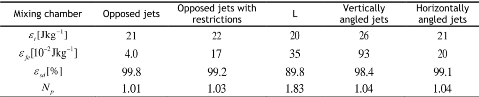
Table 2-1 Geometric parameters from experimental Work done by Sebastian and Boukobbal (1986) ...21 Table 2-2 heating system dimensions, regarding Figure 2-36 ...39 Table 3-1 Main Dimensions of the different mixing chamber’s studied ...52 Table 3-2 Inlet Velocities ...53 Table 3-3 Fluid’s properties ...54 Table 3-4 Energy dissipation for different geometries for different Re ...60
Table 3-5 ―Pancake‖ area, for several geometries at *
2
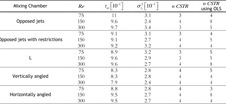
...61 Table 3-6 Fluid properties ...90 Table 3-7 CFD values for the different chambers ...90 Table 3-8 Total Energy and Friction Energy for the different chamber ...91 Table 3-9 First and second moment for the different geometries for different Re ...95
Table 3-10 Construction material compatibility, advice seals and couplings methods for the used fluids ... 105 Table 3-11 Pumps characteristics ... 106 Table 3-12 Polyurethanes dosing Pump’s type and price ... 106 Table 3-13 Transfer functions based on Sundaresan and Krishnaswamy (1978) model .... 110 Table 3-14 PID parameters for the temperature control ... 110 Table 3-15 Glycerol solution viscosities ... 117 Table 3-16 PID parameters for the temperature control ... 120 Table 3-17 Nitrogen requirements for each operation ... 121 Table 4-1 – Raw materials properties ... 132 Table 4-2 Processing Conditions ... 133 Table 4-3 Boundary conditions for the CFD simulation ... 134 Table 4-4 Frequency energy and power spectra for experimental and CFD data,
measured from ... 140 Table 4-5 Polar diameter for proposed flow structures obtained from experimental and
CFD, for stoichiometry 1:1.02 ... 142 Table 4-6 Rencast FC52 raw Material properties ... 151 Table 4-7 Processing conditions for Rencast FC52 ... 151 Table 4-8 Process characteristics time ... 153 Table 4-9 Material Properties ... 159 Table 4-10 Specimens Dimensions ... 170 Table 4-11 Mean, standard deviation and lower and upper limits of confidence of 97.5%
for the tensile test ... 175 Table 4-12 Mean, standard deviation and lower and upper limits of confidence of 97.5%
for the compressive test ... 176 Table 4-13 Mean, standard deviation and lower and upper limits of confidence of 97.5%
for the compressive test ... 177 Table 4-14 Mean, standard deviation and lower and upper limits of confidence of 97.5%
for the flexural strength and modulus ... 179 Table 5-1 Geometrical parameters and injection velocity ... 203 Table 5-2 Physical properties of the fluids ... 203 Table 5-3 Geometrical parameters ... 205 Table 5-4 Physical properties ... 205 Table 5-5 Geometric dimensions for contraction and expansion geometry ... 208 Table 5-6 Main Variables over a contraction in RIM injection ... 210
Table 5-7 – Dimensionless Factors’ and calculations ... 210 Table 5-8 Leading coefficient and exponential values for Fr number dependency in 2:1
contraction flow. ... 251 Table 5-9 Leading coefficient and exponential values for
Re
number dependency in 2:1contraction flow. ... 253 Table 5-10 Leading coefficient and exponential values for
We
number dependency in2 :1 contraction flow. ... 255 Table 5-11 Leading coefficient and exponential values for Fr number dependency in
2 :1 expansion flow. ... 256 Table 5-12 Leading coefficient and exponential values for
Re
number dependency in2 :1 expansion flow. ... 257 Table 5-13 Leading coefficient and exponential values for
We
number dependency in2 :1 expansion flow. ... 259 Table 5-14 Examples of flow pattern and corresponding color ... 260 Table 5-15 Solutions for pressure drop over a length, L , for different cross sections
(White, 2006) ... 267 Table 5-16 Constants for kinetic models ... 271
Notation
NCO
NCO concentrationA
Area 2[m ] v
A
Air entrapped area 2[m ]
B Body forces tensor [N]
b Width [m]
c Distance to the neutral plane [m] Ca Capillary number
p
c Specific heat capacity -1 -1
[Jkg K ]
d Injector diameter [m]
c
d Cell diameter [m]
D Mixing chamber diameter [m]
D Deformation tensor 1
D
Inlet thickness [m]2
D
Outlet thickness [m]dA Area’s normal vector 2
[m ]
E Total Energy [J]
e Total energy per mass -1
[Jkg ] '
E
Storage modulus [Pa]''
E
Loss modulus [Pa]a
E
Activation energy -1[Jmol ]
C
E
Compressive modulus [Pa]f
E Total work of friction [J]
i
E
Young Modulus [Pa]
rE t Residence Time Distribution F Free energy
[J]
inj F Injection force[N]
f Admissible displacement[m]
bd f Bending displacement[m]
sh f Shear displacement[m]
r F t Tracer output mF
Mass flux nF
Cumulative distribution functionn
f
Natural frequency [Hz]n
f
Density distribution functionF
r Flow rate ratioST
F
Force at interfacial surface[N]
g Gravity [ms ]2g Gravitational acceleration vector [ms ]2
xx
G
Power spectraH Mixing chamber length [m] h Specific enthalpy -1
[kJkg ]
i
h
Convective heat transfer coefficient of fluid i -2 -1[Wm K ]
m
H
Mould height [m]s
H
Initial specimen height [m]r
H
Heat released [J]I Cross-sectional beam moment of inertia [m ]4
I Identity tensor
J Diffusion flux vector
j
Position along inlet surface [m]k Specific velocity of reaction [Jmole K ]-1 -1
also, thermal conductivity -1 -1
[Wm K ]
i
K
Thougness -3[Jm ]
D
K
PID derivative term KE Kinetic energy [W]r
KE
Kinetic energy ratioI
K
PID integral termp
K PID proportional term
steel
k
Steel thermal conductivity -2 -1[Wm K ]
sc
k
surface curvature radiusl Impingement point position [m] *
l
Non dimensional Impingement point L Length [m]m Mass [kg]
m Mass flow rate -1
[kgs ] M Torque [Nm] r
M
Momentum ratioN
Nozzle length [m] n Number of reactorsn
Normal vector pN
Power number P Power [W] p Pressure [Pa]p Pressure tensor [Pa]
inj
p Injection pressure [Pa]
PE Pressure energy [W] q Volumetric flow rate -1
q Heat flux -2 [Wm ]
Q
Heat [J] tQ
Transferred heat [J]R
Part radius [m]also, square sum of deviation
also, Universal Gas Constant -1 -1
[Jk mol ]
r
Injector radius [m]r Position [m]
R r
Correlation of volume fractionRe Reynolds number s Striation thickness [m] St Strouhal number d
s
Standard deviation lS
Linear shrinkage ls
Scale of segregation wS
Thickness shrinkage T Temperature[°C]
T Traction forces tensor [N]
t
Time [s]also, Thickness [m] 0.975
t
t-Student parameter97.5%
av
t
Average residence timecure
t Cure time [s]
d
t Dark structure thickness [m]
d
T Deflection Temperature
[°C]
extraction
t Extraction time [s]
g
T Glass transition temperature
[°C]
gel
t Gel time [s]
r
t
Normalize residence timer
T
Thickness ratioTan
Damping factor u Internal energy [J]also, PID output
U Overall heat transfer coefficient -2 -1
[Wm °C ] v Velocity vector -2 [ms ] p
V
PTD [V]V
Volume 3 [m ] W Work [J] w Deflection [m] We Weber numberx
Space coordinate [m]g
X
Glycerine fraction y Space coordinate [m] z Space coordinate [m] Greek letters
Fraction conversion i
Volumetric fraction of phase ig l
Surface tension between phase gas and liquid [Nm ] -1inj
Strain rate at injector walls -1
[s ] r
H
Released heat [J] *p
Normalized differential static pressurep
Differential static pressure [Pa]t
Time step [s]
ad
T
Adiabatic temperature rise[°C]
x Numerical grid element length [m]
Internal walls thickness [m]
Strainfe
Friction energy dissipation 1[Jkg ]
se
Shear energy dissipation 1[Jkg ]
sd
Shear dissipation 1[Jkg ]
t
Total energy dissipation 1[Jkg ]
tot
Energy dissipation rate [W]
Surface Equationg
Volumetric efficiency Rate of energy production per unit mass -1
[Wkg ] Angle [rad]
Contraction coefficient
Viscosity [Pa s]
Kinematic viscosity 2 -1 [m s ]
Non-dimensional rate of strain
Density -3[kgm ]
σ Normal stress Tensor [Pa] 2
r
t
non-dimensional variance of RTDB
Break strength [Pa]
f
Flexural strength [Pa]M
Maximum strength [Pa]
y
Yield strength [Pa]
Passage time [s] also, Shear stress [Pa]τ Stress tensor [Pa]
Velocity -1
Induced frequency [Hz]r
Diameter ratio
Empirical loss coefficient Stream function -1 [m s ]2 *ω
Non-dimension vorticity Mathematical operators
d
dt
Time derivative
Gradient operator( )
Curl operator
Divergence operator
D Dt substantial derivate
2 Laplacian operator
T Transpose
Avarage
norm Subscripts Flow 0 Initial 1 Left injector 2 Right injector 3 Outlet a Air A Species Ab Bottom of mixing chamber bd Bending
c
Compressive cm Center of masscr
CriticalCS
Control surfacecs
Cross-sectionalCV
Control Volume d Dryds
Downstreame
Control surface ext a Exterior-airext o
Exterior-oilg
Gas f Flexuralfl
Fluidfr
Frictionfs
Flow section i Species indexin Inlet inj At injector
int Interior
iso Isocyanate
k Refer to surrounds
l Lateral of mixing chamber
liq
Liquidmax
Maximum valueo Oil
d
o
Dry part of oilw
o
Wet part of oilout Outlet pol Polyol
r
Rooms
Shaftsh
Shear t Tensiletop Top of the mixing chamber
us Upstream
w
Wall we Wetx
x
component of variable y y component of variablez
zcomponent of variable Abreviation1½D One-dimensional and half 2½D Two-dimensional and half 3D Three-dimensional
ALE Arbitrary Lagrangean-Eulerian
ASTM Americam Society for Testing Materials CAD Computeded Aided Design
CDRsp Centro para o Desenvolvimento Rápido e Sustentado do Produto CFD Computational Fluid Dynamics
CNC Computational Numerical Command CVFEM Control Volume Finite Element Method DMA Dynamical Mechanical Analyzer
DPT Differential Pressure Transducer FDM Finite Difference Method
FEM Finite Element Method
FEUP Faculdade de Engenharia da Universidade do Porto FVM Finite Volume Method
IPLeiria Instituto Politécnico de Leiria ISO International Standard Organization LDA Laser Doppler Anonemetry
LIF Laser Induced Fluorescence
LSRE Laboratory of Separation and Reaction Engineering MAC Marker-And-Cell
PID Proportional Integrate Derivative PIV Particle Image Velocimetry PIT Particle Image Thermometry PTV Particle Tracking Velocimetry
RIM Reaction Injection Moulding RIMcop®
Reaction Injection Moulding with Control of Oscillation and Pulsation RRIM Reinforced Reaction Injection Moulding
RTD Residence Time Distribution SEM Scanning Electron Microscopy
SRIM Structural Reaction Injection Moulding TIM Thermoplastic Injection Moulding VOF Volume of Fluid
1 Introduction
1.1 Reaction Injection Moulding
Reaction Injection Molding (RIM) is a molding process consisting in the mixture of two or more raw materials’, generally a polyol and an isocyanate, originating a Polyurethane. The mixing occurs in a mixing chamber followed by the injection of the reacting mixture of the two monomers into a mold. The RIM processes takes place at low pressure and temperature, when compared with Thermoplastics Injection Molding (TIM), due to the low viscosity of the monomers and of the reacting mixture of the monomers that solidifies inside the mold, originating a polymer part (see Figure 1-1).
Mixing in RIM can be promoted in two different ways: by stirring, using a static or dynamic mixer with several geometries and sizes – this is called low pressure RIM; or by impingement mixing, where two or more raw materials are mixed as opposed jets that impinge each other inside a mixing chamber at a high velocity, normally in the range between
10
to -1100ms (Santos et al., 2005). The process with a stirrer is called low pressure RIM and the process with impinging jets is called high pressure RIM. The mixing chamber is, usually, cylindrical with 10mm diameter, with two or more nozzles, with
1
to3mm
of diameter. The mixing phase is the only difference between high pressure RIM orlow pressure RIM.
After the mixing phase, the mixture is injected into a mold. Inside the mould cavity the reacting mixture flows at low pressure, temperature and viscosity. The polymerization, called cure reaction, occurs in the mold, where the material solidifies also at low pressure and temperature. This is an exothermic and a fast process, requiring less energy than injection of other types of polymeric materials (Teixeira, 2000).
It is possible to determine four or five distinct phases, depending on final part’s quality requirements in the RIM process:
the mixing of low viscosity monomers in the mixing chamber; the mold filling;
the polymerization or cure reaction; the part extraction;
eventually, post-cure operations to achieve better properties.
The mixing phase has a major impact on the final quality of the parts, since there is a relation between mixing and the extent of the polymerization reaction and as a consequence on the mechanical properties of the formed polymer properties. The mixing phase is short, and heavily relies on the hydrodynamics inside the RIM mixing chamber. After the mixing, the reacting mixture of monomers is injected into a mould, with a flow regime that should be as close to laminar regime as possible to avoid air bubbles entrapment and other parts defects. The mould should be totally filled before the viscosity increase due to the chemical reaction will cause a huge increase on the filling pressure. This viscosity increase rate is determined by the kinetics of the polymer curing. During the polymerization the mechanical properties, the transition temperature and the molecular weight of polymers increase. The cure reaction is exothermic, releasing a considerable amount of heat and promoting heat transfer between part and mould material. Due to this heat transfer and cure reaction, there are expansion and contraction phenomena, promoting residual tensions on the part. In order to avoid these residual tensions, the mould designers should project a proper cooling system. This phase and
phenomena are shown, over the moulding cycle, in Figure 1-2 (Bártolo and Mateus, 2003; Martinho et al., 2003).
Figure 1-2 Phenomena associated to the different stages in RIM(Bártolo and Mateus, 2003)
In Figure 1-3 are shown the cycle times associated to the RIM process. From this figure is possible to concluded that most of the cycle time is spent in the cure reaction inside the mould (
60%
of total time). Post-moulding operations uses20%
, and opening and closingthe mould account for
10%
of the cycle time. The filling time corresponds to1% of the
total cycle
, although, this time depends on the chemical system used, the part thicknessand on the mould and cooling system design (Bártolo and Mateus, 2003; Martinho et al., 2003).
The utilization of low viscosity materials (in the range of
10
a1500mPa s
), the lowprocessing temperature and the low pressure required for filling (up to
30bar
) are the thebasis of the major advantages of RIM over other polymer injection processes, namely TIM. The low pressures and temperatures allow simpler and less resistant moulds, and thus construction materials other than steel can be employed, an in addition to this less usual fabrication technologies, such as Rapid Manufacturing techniques, can be used (Bártolo and Mateus, 2003). This lead to economic advantages, since the equipment price is lower and also the energy consumption is lower (Bártolo and Mateus, 2003). Another advantage is the injection of bigger parts (until 50kg), with high complexity and large thickness variation without affecting the final quality. RIM also enables the injection of parts with metallic inserts, thinner walls and A Class surfaces (Bártolo and Mateus, 2003; George, 2000). Besides, it is possible to inject a huge range of materials with RIM, some of them with similar properties to thermoplastics, such as polycarbonate and ABS. The RIM material show high chemical resistance, and the manufactured parts show good resistance to organic and inorganic acids and a higher resistance to ageing (Bártolo and Mateus, 2003; Martinho et al., 2003).
On the other hand, some RIMs characteristics that are related with the advantages, also present disadvantages in industrial projects: the low viscosity of materials causes difficulties in mould seals, the resin can adhere to mould surface and if the filling is too fast, can create air bubbles or other defects. The low mould filling pressure introduces difficulties on removing air bubbles, mainly in corners or over inserts. If the filling is slower than curing, which could occur due to the usage of highly reactive materials, this could originate a short shot, where the mould is not totally filled (Macosko, 1989).
Intrinsic characteristics of the RIM, enables the processing of a wide variety of materials, where some reinforcements can be placed. Macosko (1989) points that half of the materials processed in RIM have fillers. Several fillers can be used, being the most common ones the mineral fibers that could be milled, flakes or continuous fibers (Bártolo and Mateus, 2003). Depending on the type of fiber the process can be classified as Reinforced RIM (RRIM) or Structural RIM (SRIM). The RRIM consist in mixing the fiber, or another type of filler, in one of the raw materials. The reinforcement filler, normally has small dimensions (between
0.4
to1.5mm
), which enables the dosing and pumping directlyinside the mould (Bártolo and Mateus, 2003). Relatively to SRIM, the fiber is placed inside the mould, and after the resin is injected into the moulds, a pre-formed layout of the fiber is impregnated with the resin (Bártolo and Mateus, 2003).
1.2 Relevance and Motivation
The Reaction Injection Moulding is a process for the production of parts with a wide range of applications and, until today, RIM has relevant utilization in low and medium size series. Despite the industrial relevance and advantages of the process, RIM is not so-well studied and so there is plenty of room to enhance this process and solve a number of operational issues, which is the main aim of this research work.
This thesis was framed within the scope of a joint project on RIM between LSRE-FEUP and CDRsp-IPLeiria, funded by Fundação da Ciência e Tecnologia: ―Reaction Injection Moulding (RIM): Controlled Mixing and Novel Design Concepts in a New Prototype Machine‖, REF: PTDC/CTM/72595/2006. This project was the follow-up of other projects on RIM, either at LSRE, and CDRsp. This thesis covers the previous work that was done by these two distinct research groups, LSRE-FEUP and CDRsp-IPLeiria, in different but complementary fields of the RIM technology.
The first part of the work will focus on the new technology RIMcop. This technology was patented and it was based on knowledge gathered from previous studies on the hydrodynamics in the RIM machine mixing head, namely on the results from the PhD theses of Teixeira (2000) and Santos (2003).
Teixeira (2000) studied the flow field experimentally using a Laser Doppler Anemometry (LDA) technique, and Computational Fluid Dynamics (CFD). The computational work was done with a 2D model of the RIM mixing chamber, and was the first computational approach to the study of the flow dynamics in RIM.
Santos (2003) studied the dynamic behavior of flow field, its dependence on the operational and some design parameters of the mixing chamber, using both LDA and CFD tools. Furthermore, using Particle Image Velocimetry (PIV), Santos (2003) observed and proposed the flow structures formed inside the RIM Mixing Chamber.
In the second part of this work, the use of CFD tools on the definition of rules for the design of RIM moulds will be studied. The knowledge of the behavior of polymeric flowing materials inside the mould cavity is a powerful tool on the design of RIM moulds, which can reduce the part rejection rate due to poor mould design. Presently, the mould design for thermoplastics is widely studied by several groups, who introduced concepts and project rules (Knipp, 1998). On the other hand, for the reactive polymers, and particularly, for polyurethanes, the available literature is scarce, and the few available guidelines are from private companies and it mainly is based on empirical approaches (Torcato et al., 2011). Another major motivation behind the present work, is to contribute on the methodologies
for RIM moulds design, which could contribute to an increase of the RIM technology share in the plastics injection market.
1.3 Thesis Objectives and Layout
This work intends to study several steps of the RIM process from mixing to mould design. The main goals of this study were the design of a new mixing head based on the patented RIMCop technology (Lopes et al., 2005), assess the mixing quality of the RIMCop technology for a polyurethane system and set rules for the design of RIM moulds. CFD tools were used for comparison between commercial solutions for RIM mixing heads, and to study the mould filling in RIM for characteristic geometry features of moulds. The implementation of the RIMcop technology in industrial prototype equipment enabled a better insight into the effect of mixing in RIM on the mechanical properties of the processed material.
The thesis goals are addressed following this structure:
Chapter 2 sets the state-of-art in RIM mixing chambers, from the first commercial mixing heads of Keuerleber and Pahl (1972) up to the RIMcop technology introduction (Lopes et al., 2005). This chapter also describes the different methods used for undirected mixing analysis in RIM. Chapter 2 also reviews the state-of-art of project rules for mould design in RIM.
Chapter 3 focus on the project of machines with RIMCop technology. This chapter introduces the actual project of the RIMCop pilot machine built at LSRE-FEUP. In the first section, a comparative study of several mixing geometries, used at commercial equipment, is made. The second section presents the two pilot RIM machines used along this work at CDRsp-IPLeiria and LSRE-FEUP. The equipment at LSRE-FEUP introduces the novel mixing control technology denominated RIMCop. The last section introduces the calibration and preparation of the RIM equipment for proof of concept of the RIMcop technology.
Chapter 4 provides details on the RIMCop technology usage. In this chapter, opposed mixing chamber RIM moulding and RIMCop technology were used to produce PU parts. In the first part of the chapter, the mechanical properties of RIM moulded part are assessed. The second part of Chapter 4 introduces the results from the application of RIMCoptechnology on the processing of the PU part, namely on the effect of the opposed kinetic energy ratio as a process control variable.
Chapter 5 presents a 2D and 3D VOF model for mould filling simulation in Reaction Injection Moulding, which tracks the flow filling front. Using the model, several simulations were run to identify the phenomena that occur during the RIM mould filling flow, and the effect of several fluid mechanics parameters. From this study, a flow map was created to help the decision based on inertial, viscous, gravitical and superficial forces. The last part of the chapter, introduces some rules for RIM moulds design, covering the project, filling and extraction operations.
Finally, the last chapter condenses the results and knowledge developed in course of the present work. Future steps, related with present work, are suggested.
1.4 References
Bártolo, P., Mateus, A., 2003. Moldação por Reacção a Baixa Pressão (RIM - Reaction Injection Moulding). Molde 57, 32-37.
George, H., 2000. Reaction Injection Molding(RIM) Technology - New Horizons. Tucson, Fall Meeting of Polyurethane Manufacturing Association.
Keuerleber, R., Pahl, F., 1972. Devide for feeding flowable material to a mold cavity. Patent US3706515.
Knipp, U., 1998. Molds for Polyurethanes Products, in: Stoeckhert, K., Menning, G. (Eds.), Mold-Making Handbook. Hanser Publishers, Munich, Germany.
Lopes, J.C.B., Santos, R.J., Teixeira, A.M., Costa, M.R.P.F.N., 2005. Production Process of Plastic Parts by Reaction Injection Moulding, and Related Head Device. Patent WO 2005/097477.
Macosko, C., 1989. RIM Fundamentals of Reaction Injection Molding. Hanser Publishers, Munich, Germany.
Martinho, P., Mateus, A., Bártolo, P., Bolrão, J., Gaspar, J., Ferreira, P., 2003. Utilização integrada de Técnicas Avançadas para Análise e Optimização do Processo RIM. O Molde 58, 43-49.
Santos, R.J., 2003. Mixing Mechanisms in Reaction Injection Moulding - RIM - An LDS/PIV Experimental Study and CFD Simulation, Ph.D. Thesis, Deparment of Chemical Engineering, Universidade do Porto, Porto.
Santos, R.J., Teixeira, A.M., Lopes, J.C.B., 2005. Study of mixing and chemical reaction in RIM. Chemical Engineering Science 60, 2381-2398.
Teixeira, A.M., 2000. Escoamento na Cabeça de Mistura de uma Máquina RIM, Ph.D. Thesis, Deparment of Chemical Engineering, University of Porto, Porto.
Torcato, R., Santos, R., Dias, M., Olivetti, E., Roth, R., 2011. Concurrent Development of RIM Parts, in: Frey, D.D., Fakuda, S., Rock, G. (Eds.), 18th ISPE International Conference on Concurrent Engineering. Springer-Verlag, Boston.