Repositório ISCTE-IUL
Deposited in Repositório ISCTE-IUL:
2018-04-19
Deposited version:
Post-print
Peer-review status of attached file:
Peer-reviewed
Citation for published item:
Ramos, T. R. P., Morais, C. S. & Barbosa-Póvoa, A. P. (2018). The smart waste collection routing problem: alternative operational management approaches. Expert Systems with Applications. 103, 146-158
Further information on publisher's website:
10.1016/j.eswa.2018.03.001
Publisher's copyright statement:
This is the peer reviewed version of the following article: Ramos, T. R. P., Morais, C. S. & Barbosa-Póvoa, A. P. (2018). The smart waste collection routing problem: alternative operational
management approaches. Expert Systems with Applications. 103, 146-158, which has been published in final form at https://dx.doi.org/10.1016/j.eswa.2018.03.001. This article may be used for non-commercial purposes in accordance with the Publisher's Terms and Conditions for self-archiving.
Use policy
Creative Commons CC BY 4.0
The full-text may be used and/or reproduced, and given to third parties in any format or medium, without prior permission or charge, for personal research or study, educational, or not-for-profit purposes provided that:
• a full bibliographic reference is made to the original source • a link is made to the metadata record in the Repository • the full-text is not changed in any way
The full-text must not be sold in any format or medium without the formal permission of the copyright holders. Serviços de Informação e Documentação, Instituto Universitário de Lisboa (ISCTE-IUL)
Av. das Forças Armadas, Edifício II, 1649-026 Lisboa Portugal Phone: +(351) 217 903 024 | e-mail: [email protected]
1
The Smart Waste Collection Routing Problem: alternative operational
management approaches
Tânia Rodrigues Pereira Ramos*
Centre for Management Studies, Instituto Superior Técnico (CEG-IST) Universidade de Lisboa
Av. Rovisco Pais, 1049-001 Lisbon, Portugal Business Research Unit, ISCTE (BRU-ISCTE)
Instituto Universitário de Lisboa
Av. Das Forças Armadas, 1649-026 Lisbon, Portugal
Carolina Soares de Morais
Centre for Management Studies, Instituto Superior Técnico (CEG-IST) Universidade de Lisboa
Av. Rovisco Pais, 1049-001 Lisbon, Portugal
Ana Paula Barbosa-Póvoa
Centre for Management Studies, Instituto Superior Técnico (CEG-IST) Universidade de Lisboa
Av. Rovisco Pais, 1049-001 Lisbon, Portugal
*Corresponding Author:
Tânia Rodrigues Pereira Ramos [email protected]
Address: Av. Rovisco Pais, 1049-001 Lisbon, Portugal Phone Number: +351 21 841 9956
2 The Smart Waste Collection Routing Problem: alternative operational management
approaches
Abstract: Waste collection is nowadays an increasingly important business. However, it is often an inefficient operation due to the high uncertainty associated with the real waste bins’ fill-levels. To deal with such uncertainty the use of sensors to transmit real time information is seen as possible solution. But, in order to improve operations’ efficiency, the sensors’ usage must be combined with optimization procedures that inform on the optimal collection routes to operationalize, so as to guarantee a maximization of the waste collected while also minimizing transportation costs. The present work explores this challenge and studies three operational management approaches to define dynamic optimal routes, considering the access to real-time information on the bins’ fill-levels. A real case study is solved and important results were found where significant profit improvements are observed when compared to the real operation. This shows the potential of the proposed approaches to build an expert system, which can support the operations manager’s decisions.
Keywords: Real-Time Data; Sensors; Smart Collection; Optimization; Waste Management; Dynamic Routing
1. Introduction
The Internet-of-Things (IoT) is an emergent research topic that is causing a positive impact in the way operations are managed (Atzori et al., 2017). With this in mind, companies are developing the capabilities needed to explore the use of Information and Communication Technologies (ICT). These will potentiate higher efficiency and a better effectiveness of their operations (Daugherty et al., 2005; Oliveira et al., 2015), while enhancing the organizations’ adjustment to today’s dynamic environment (Fayoumi and Loucopoulos, 2016). In this set, the necessary conditions to develop dynamic expert systems able to explore real-time information to inform the organizations’ practice and improve their operational decision-making are available. One of the areas where such conditions should be investigated is the waste management area where real-time information on bins’ fill-levels, provided by volumetric sensors installed in waste containers should be explored, as defined in the development of Smart Cities (Gruler et al., 2017). This access to real-time information on the bins’ fill-levels, if effectively used by operations managers, could result in an improvement of productivity. This will have a high impact not only on the company’s profit, but also on society’s welfare, since waste management is an important problem in global economies today. Urban populations and consumption patterns are increasing (UNEP, 2013), generating ever-growing waste levels that needs to be collected and treated. As an example, during 2015, around 477 kg of municipal waste per capita were generated in Europe (Eurostat, 2017), representing tons of waste that had to be collected every day, implying collection truck coverages of several kilometers with consequent thousands of Greenhouse Gases emissions that should be minimized.
3 Waste collection companies face, every day, in their operation, high transportation costs and, more importantly, high inefficient usage of their resources, as trucks often visit waste bins that are only partially full. As stated by Nuortio et al. (2006), the amount of municipal solid waste is highly variable and the accumulation of waste depends on several factors. Consequently, bins’ fill-levels are difficult to forecast. From published data on a Portuguese waste collection company, it was observed that within a period of 6 months, only 40% of the recyclable waste bins were collected with a fill-level higher than 75% (Gonçalves, 2014). This is, unfortunately, a common situation in waste management systems. To overcome this problem, efficient waste collection systems should be operated, where the role of in-place expert systems could represent a major cornerstone that would help to define optimal operational management procedures.
In this context, the access to bins’ fill-levels in real-time, through monitoring systems, emerges as a path to be explored, as this will allow the reduction of demand uncertainty (e.g. the amount of real waste level in the bins). However, accessing this data is not enough, and to increase a waste collection operation’s efficiency, such data should be also used accordingly to optimize the collection routes. Consequently, the development of routing models that would explore the information provided by monitoring technologies should then be pursued. As stated by Faccio et al. (2011), modern traceability devices, like volumetric sensors for example, can be used to obtain real-time information that should allow for an optimization of the route plan, minimizing the covered distance, as well as the number of vehicles needed for the collection. In conclusion, we should move from the traditional waste collection operation based on a so-called “blind collection”, to a dynamic operation. In the former, bins are attended without prior knowledge of their actual fill-level through pre-defined and static routes (i.e. the same route is repeated for a given time interval), while in the latter the access to information on the bins’ real fill-levels is available and the definition of dynamic routes (rather than static routes) is undertaken. A “smart collection” is defined which, as stated by Mamun et al. (2016), can result in a significant increase of cost effectiveness. Given this setting, the research question to be answered is: “how should dynamic routes be defined if access to real-time information exists?”
The present work aims to answer to this question, and for that it compares three different operational management approaches that define dynamic collection routes considering data provided by volumetric sensors placed inside the bins: 1) a limited approach; 2) a smart collection approach; and 3) a smarter collection approach. The three approaches are compared using real data from a Portuguese company responsible for the recyclable waste collection of 14 municipalities in Portugal. For each approach, its performance is assessed through a set of key performance indicators (KPIs): distance travelled; amount of waste collected; profit; kg per km ratio; and vehicle usage rate. These KPIs are compared with the values describing the current situation (also known as “blind collection”). Additionally, the service level provided by the waste collection company to the population is also studied. Service level is here defined by the number of bins that cannot overflow. Two scenarios are tested: service level of 100% and 99%, meaning that in the prior no container can overflow while in the latter 1% of the containers may overflow. In cases where the service level established is lower than 100%, a maximum overflowing threshold must be defined to prevent containers to overflow for a long period of time.
The remainder of the paper is organized as follows: In section 2, a Literature Review on routing models combined with ICT approaches applied to waste management is presented. In section 3, the three management approaches are detailed and the mathematical models embedded in each approach are characterized. Section 4 describes the real case study and shows the results of the
4 application for each approach. Finally, section 5 concludes the paper and presents some suggestions for further research.
2. Literature Review
The advances on ICT to develop dynamic expert systems able to improve organizations’ operational decision-making in the waste management area are supported by the work of Mamun et al. (2016) and reviews of Hannan et al. (2015) and Melaré et al. (2017), where decision support systems applied to waste management using ICTs are analyzed.
Mamun et al. (2016) designed an automated bin status monitoring system that exercises a set of novel rules based decision algorithms providing a robust platform that can acquire bins’ condition data instantly, as soon as waste is thrown inside a smart bin. The system, as the authors conclude, can help to implement dynamic routing for waste collection, which may provide significant increase of cost effectiveness, one of the main drivers in Smart Cities.
Hannan et al. (2015) reviewed 23 works on data acquisition technologies, and from these, four were classified as having as target application the route/collection optimization: Johansson (2006), Apaydin and Gonullo (2007), Rovetta et al. (2009), Faccio et al. (2011). Johansson (2006) evaluated different scheduling and routing policies using a blend of analytical and simulation modelling combined with empirical case research to, firstly, construct analytical models to determine the effect of dynamic planning in a waste collection context; and secondly, build more realistic models using stochastic discrete-event simulation. The approach considers a relaxation on the assumptions made in the analytical models and considers each container being fitted with a sensor that emits an alarm signal when the container is full. A case study is solved based on observations and interviews with planners and drivers operating recycling stations in a Sweden’s city aiming to investigate their usage of real-time data. As main conclusions, the authors state that dynamic scheduling and routing policies lead to lower operating costs and shorter collection and hauling distances, with a lower number of collected containers, when compared to the data when using a static policy. Apaydin and Gonullo (2007) create a data set for a Municipal Solid Waste Collection (MSWC) by recording, through a video camera installed in the collection vehicles, the collection operation of 39 districts in the city of Trabzon - Turkey. The authors applied a GIS based Vehicle Routing model and used the software Route View ProTM, integrated with GIS elements as
an optimization tool to define collection routes. As conclusion, their work reveals that performing route optimization on current solid waste collection paths leads to a reduction in the travelled distance and in time to collection and hauling. Rovetta et al. (2009) described an application of municipal solid waste monitoring based on the combination of a distributed sensor technology and a geographical information system. The main purpose of the work was to provide information about the containers, focusing on weight and density of its content. Devices equipped with a set of sensors were applied in Pudong, Shanghai (PR China) allowing the testing and evaluation of the application. The data collected from 15 containers was treated and used in a VRP to obtain an optimized path. As conclusion, the authors sustain that the implementation of a central monitoring application would provide quantitative data on the waste inside the containers, which could then be used to establish appropriate waste management policies. Finally, Faccio et al. (2011) studied the integration of real-time traceability data with a heuristic routing model where
5 only bins that reach an imposed minimum replenishment level were visited. A real-time traceability data routing model is proposed to solve multiple objectives, such as: to minimize number of vehicles per fleet; to minimize travel time; and to minimize total distance covered. The heuristic consists of two main steps: 1) to define which bins should be collected and, 2) once defined the set of bins to be emptied, each vehicle route is optimized.
In the mentioned works, where data acquisition technologies are combined with route collection optimization, routes have been defined through classical VRP models, which consider a predefined set of bins to be collected. In traditional waste collection problems, i.e., where no data acquisition technology is involved, the decision on the bins to be collected is not explored (see reviews on waste collection as: Belien et al. (2012), Ghiani et al. (2014), and Han and Ponce-Cueto (2015)). Dynamic collection should then be further extended to attain more profitable solutions with higher resources utilization, where the definition of the set of containers to visit is to be optimized, along with route sequence. Aras et al. (2011), Aksen et al. (2012) and Anghinolfi et al. (2013) are examples of works that studied dynamic collection problems, where sites are selected to be visited taking into account their profit. However, no real-time information is considered in those works. Aras et al. (2011) studied the reverse logistics problem of a firm that aims to collect used products (referred to as cores) from its dealers with the objective of optimizing the routes of a homogeneous fleet of capacitated vehicles each of which will depart from a collection center, visit several dealers, and return to the same center. As the firm was not obliged to visit all dealers, the authors formulated two MILP models for a Multi-Depot VRP with pricing where the profit associated with each visit (revenues from cores minus acquisition price to be paid to take the cores back) is maximized. As solution approach, the authors developed a Tabu Search based heuristic method. Aksen et al. (2012) considered a biodiesel production company that collects waste vegetable oil from source points to develop two different formulations for a Selective Periodic Inventory Routing Problem. The authors compare and apply the better performing formulation on a real-world problem. In the new formulation, the source points would not be visited if not profitable. Anghinolfi et al. (2013) proposed a dynamic optimization model for the definition of waste collection routes based on a GIS-based waste generation model. Bins were grouped in three cells (macro-bins) and the paths within the cells were considered known and fixed, i.e. the sequence of bins that are emptied is a priori known. The model determined the routes to be performed that maximize the profit (revenues for collected waste minus vehicles’ costs plus costs due to the waste remaining in the cells at the end of the planning period). A very small size problem was solved where three cells, a depot and a recycling site (where all the collected materials are transported to) are considered.
When dynamic collection is coupled with real-time information, few works were identified: Mes (2012), Anagnostopoulos et al. (2015), Gutierrez et al. (2015) and Ramos et al. (2017). Mes (2012) used discrete event simulation to evaluate how dynamic planning methodologies could be best applied to collect waste from underground containers equipped with motion sensors, which counts the number of lid openings, recording how many disposals are made. The author compared a static planning methodology based on a desired time between emptying’s, with a dynamic planning, where containers are daily selected based on their estimated fill-levels. For dynamic planning, a heuristic was used, and containers were divided into MustGos (those that need to be emptied on the current day) and MayGos (those which are only included in routes if there is space left in truck capacity and working hours). The MustGos are firstly included using a cheapest insertion heuristic, and then MayGos would be inserted if space in the trucks is available.
6 A real case was solved and the author concluded that major improvements were achieved when assuming a dynamic waste collection policy. Anagnostopoulos et al. (2015) studied a dynamic waste collection architecture based on data retrieved by sensors, considering the possibility of immediate collection of high priority bins during the collection time. At first, the system defines the collection routes for the regular bins. Then, when a high-priority bin triggers an alarm (the bin becomes full or its filling rate is over to a pre-defined threshold), the system initiates the proposed routing algorithms to respond with an optimal reaction, forcing trucks to deviate from their original path to first serve the high-priority bin. Gutierrez et al. (2015) presented a waste collection solution based on the information provided by sensors installed into trashcans. The sensors transmit the trash volume data, which is then stored in a database. The selection of the cans to be daily collected is based on the historical data stored at the database through an artificial intelligence module. Every day, after the trashcans to be collected have been selected, route optimization algorithms (shortest path spanning tree, genetic algorithms and k-means) calculate the best route to follow in order to minimize driving distance. The authors use simulation to assess the dynamic system benefits, and to compare it with traditional sectorial waste collection approaches. Recently, Ramos et al. (2017) addressed the definition of dynamic routes within the waste collection problem. This work, although considering the access to real-time information, studied a simplified version of the problem in which an optimization model is solved daily considering only 68 waste bins (a small size problem). The number of available vehicles and the percentage of bins that can overflow are not considered.
Based on the above works it can be concluded that the smart waste collection routing problem is still far away from being comprehensively studied and several interesting aspects should be further addressed. At one hand, only small-size problems were tackled by optimization models, and, on the other hand, the selection of the waste bins to be emptied is only based on its weight (and not on the profit that may be attained when collecting them) and this selection step is not integrated with the routing step. Therefore, models exploring the existence of real-time information and its usage to optimize real collection routes are therefore an important research line still open that we aim to explore along this paper.
3. The Smart Waste Collection Routing Problem
3.1 Problem Description
The Smart Waste Collection Routing Problem developed here considers the use of real-time information on the bins’ fill-level to define dynamic routes.
This problem can be defined as follows: given a set of n waste bins, a set of v homogeneous vehicles and a depot (where all vehicles start and end their routes), a complete undirected graph is defined on n+1 nodes, with distances dij for each edge (i,j) in the graph. Each waste bin i has a
maximum capacity Ei. We also consider a travelling cost C per unit of distance travelled and a
revenue value R per kg of waste collected. Each vehicle has a fixed capacity Q (in kg). At the beginning of each day t, in the morning, the sensors located inside the waste bins transmit information on the bins’ fill-levels, in m3, and this information is translated into kg given the waste
density (B). To simulate the data transmitting process, two parameters are assumed for each bin i: an initial morning stock (initial stock Si), which corresponds to the data read and transmitted
7 by the sensors; and an expected daily accumulation rate ai, which is defined based on historical
data read by the sensors. To provide a certain service level to the population, a percentage of bins that can overflow (δ) is given, as well as the maximum allowed overflow threshold (ψ).
The problem in hand selects the waste bins to be visited (if any) and the optimal visiting sequence in each day t for each vehicle k , which will maximize the profit while satisfying the vehicles’ fixed capacity, the bins’ capacity and the service level defined.
3.2 Operational Management Approaches
Considering the problem description, three operational management approaches to define dynamic collection routes are studied:
1) a limited approach, based on a Cluster First-Route Second heuristic in which a minimum fill-level rule is imposed to select the bins to be attended each day. This is coupled with a Capacitated Vehicle Routing Problem (CVRP) model that optimizes each vehicle’s route, defining the best sequence to visit the selected bins;
2) a smart collection approach, in which a mathematical model is proposed to decide which bins should be visited in each day and what is the best sequence to follow, so as to guarantee maximum profit;
3) a smarter collection approach, in which a heuristic method is proposed to decide the best days to perform the collection operation according to the service level established, and the mathematical model defined in approach 2) is applied for the chosen days.
The first approach is based on the approach followed by Faccio et al. (2011), where the selection of the bins to be visited in each day is based on a minimum fill-level threshold. In this approach, a heuristic procedure is used to select the bins to be collected in each day. Once the set of bins to be visited is defined, each vehicle route is optimized through a CVRP model. In the smart (second and third) approaches, the set of containers to be visited is defined by a mathematical model, which considers the containers “attractiveness”, meaning their fill-levels. A Vehicle Routing Problem with Profits (VRPP) model is developed, aiming at the objectives of maximizing the quantity of waste collected, while minimizing the total distance travelled. Such objectives are translated into profit maximization, defined as the difference between revenues obtained from the waste collected and the transportation costs of collecting that waste. This is attained by considering that recyclable waste has a price market. For a comprehensive survey on VRPP, read Archetti et al. (2014). The above approaches are detailed in the next sections.
3.2.1 Limited Approach
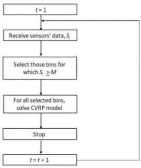
Considering an operational decision level, the routes to be completed on day t are decided in the morning of the same day t, after receiving the real-time information on the bins’ fill-level (Si). As
shown in Figure 1, the first step is to apply a simple heuristic procedure to define the bins that must be visited. This heuristic uses an imposed minimum fill-level M above which bins must be visited. Thus, all waste bins that have a Si ≥ M are considered for the routing phase. Once the set
of bins that must be emptied is defined, a CVRP model is run to optimize routes, determining the best sequence for visiting all the selected bins. This procedure is repeated for each day t.
8
Figure 1: Limited approach.
In this approach, and since the waste bins are selected in the first phase, the second phase objective is narrowed to minimize the transportation costs. The routes’ definition is performed through the mathematical formulation proposed by Baldacci et al. (2004) for the CVRP, which is adapted here to the waste collection context. The two-commodity flow formulation uses two flow variables, yij and yji, to model the flow of waste carried by a vehicle when traversing an edge (i,j).
If a vehicle travels from i to j, then the flow yij represents the load of the vehicle and the flow yji
represents the empty space on the vehicle (i.e., yij + yji = Q). Then, each route is defined by two
paths: one path from node 0 (real depot) to node n+1 (copy depot, which is a replica of the real depot) is given by the flow variables representing the vehicle load (yij); and the second path from
node n+1 (copy depot) to node 0 (real depot) is given by the flow variables representing the empty space in the vehicle (yji). This is represented in Figure 2.
Figure 2: Two-commodity flow formulation representation.
This model can be described as follows: Index sets
I = {0, 1, 2, … , n+1}: set of n waste bins and the real depot 0 and the copy depot n+1 Parameters
K: number of available homogeneous vehicles Q: vehicle capacity (in kg)
9 dij: distance between node i and node j (in km)
C: travelling cost per distance unit (in €) B: waste density (in kg/m3)
Si: amount of waste in kg at bin i (calculated using the information given by the sensor (in m3) and
the waste density (in kg/m3))
Decision variables
xij: binary variable indicating if edge (i,j) is visited, (i,j Є I)
yij: positive variable representing the flow between node i and node j, (i,j Є I)
Model
)
(
5
.
0
min
) ( ,C
d
x
T
I i j I j i ij ij
(1) s.t.
) ( ,}
1
,
0
{
\
,
2
)
(
i j I j i ji ijy
S
i
I
n
y
(2)
1 , 0 \ \{0, 1} 1 n I i i I n i inS
y
(3)
1 , 0 \ \{0, 1} 1 n I j i I n i j nQK
S
y
(4)
1 , 0 \ 0 n I i iQK
y
(5)
1 , 0 \ 00
n I j jy
(6)
) ( ,}
1
,
0
{
\
,
2
j i I i ijj
I
n
x
(7) j i I j i Qx y yij ji ij, , , (8)
i j I i j xij 0,1, , , (9)j
i
I
j
i
y
ij
,
,
,
(10)The objective function (1) considers the minimization of the transportation cost T. Given that we are using a two-commodity flow formulation, where two paths define a route, each edge is counted twice, therefore the total distance has to be multiplied by 0.5 to assess the actual distance. Constraint (2) ensures that the outflow minus the inflow at each bin is equal to twice the amount of waste present in each bin, since this formulation considers the existence of two flows passing through a node. Constraint (3) ensures that the total inflow of the copy depot is equal to the total amount of waste in the bins, while constraint (4) ensures that the total outflow of the copy depot is equal to the residual capacity of the vehicle fleet. Constraint (5) guarantees that the total inflow of the real depot is lower or equal to the capacity of the vehicle fleet and constraint (6) completes this by guaranteeing that the total outflow of real depot is equal to zero. The existence of two
10 edges incident to each bin is ensured by constraint (7). Constraint (8) links variables x and y, guaranteeing that the sum of the flows for every edge (i,j) must be equal to the vehicles’ capacity if the edge is traversed by a vehicle. Finally, the variables’ domain is given in constraints (9) and (10).
3.2.2 Smart Collection Approach
The Smart Waste Collection Routing (SWCR) approach performs, in an integrated way, the choice of the bins to be visited each day and the best sequence to collect them while guaranteeing the maximum profit. Here, the service level offered to the population is considered given a percentage of bins that may overflow (δ) and a maximum overflowing threshold (ψ) to guarantee that the same bin does not continue to accumulate waste without being collected for a long period of time. This maximum overflowing threshold represents a maximum usage of the bins’ capacity. In this model, the number of vehicles to be used is a decision variable and there exists a penalty for its utilization, Ω, forcing the model to allocate to the operation the least possible number of vehicles. No minimum imposed limit rule is used in this model to select the bins to be attended, as in approach 1).
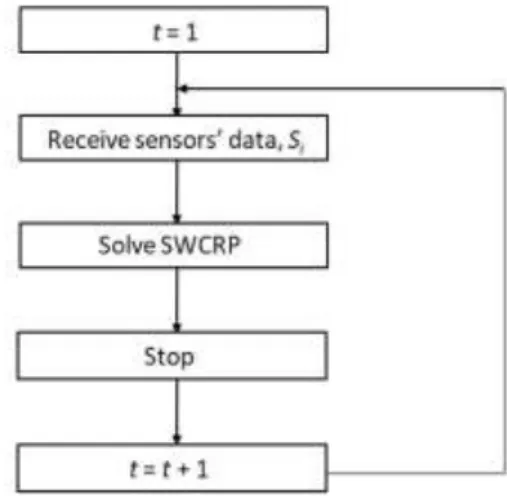
Considering an operational decision level, the routes to be performed at day t are decided in the morning of day t, after receiving the real-time information on the bins’ fill-level, as shown in Figure 3. The model is run every morning, defining the sequence of bins to be visited for each day, considering the ones that are worth to be collected given its fill-level and the transportation cost incurred to collect them.
Figure 3: Smart Collection approach.
For solving the SWCRP, a MILP model is developed. This is based on the two-commodity flow formulation proposed by Baldacci et al. (2004), which is adapted and extended to the smart waste collection scenario.
Index sets
I = {0, 1, 2, … , n+1}: set of n waste bins and the real depot 0 and the copy depot n+1 Parameters
11 R: selling price per kg of a recyclable material (in €)
Ω: penalty for the use of the vehicles (in €) Q: vehicle capacity (in kg)
B: waste density (in kg/m3)
dij: distance between node i and node j
Si: amount of waste in kg at bin i (calculated using the information given by the sensor (in m3) and
the material density (in kg/m3))
ai: expected daily accumulation rate of bin i (in kg)
Ei: capacity of bin i (in kg)
H: number of waste bins for which Si + ai > Ei
δ: percentage of bins that can overflow, considering the service level to be offered ψ: maximum bins overflowing threshold allowed
Decision variables
xij: binary variable indicating if edge (i,j) is visited, (i,j Є I)
yij: positive variable representing the flow between node i and node j, (i,j Є I)
gi: binary variable indicating if waste bin i is visited, (i,j Є I\{0,n+1})
k: integer variable on the number of vehicles to use
Model
(
0
.
5
(
)
)
max
1 , 0 \
,( )
n I i i I j I j i ij ij i ig
C
x
d
k
S
R
P
(11) s.t.(6), (8) and
) ( ,}
1
,
0
{
\
,
2
)
(
i j I j i i ji ijy
S
g
i
I
n
y
(12)
1 , 0 \ \{0, 1} 1 n I i i I n i i inS
g
y
(13)
1 , 0 \ \{0, 1} 1 n I j i I n i i j nQk
S
g
y
(14)
1 , 0 \ 0 n I i iQk
y
(15)
1 , 0 \ 00
n I j jy
(16) n Sigai Ei H n
I i i
\0, 1: (17)
i i ii
I
n
S
E
g
1
,
\
0
,
1
:
(18)
) ( ,}
1
,
0
{
\
,
2
j i I i i ijg
j
I
n
x
(19)
i
j
I
i
j
g
x
ij,
i
0
,
1
,
,
,
(20)12
j
i
I
j
i
y
ij
,
,
,
(21)
k
(22)The objective function (11) considers the maximization of profit (P), defined as the difference between the revenues from selling the waste collected and the transportation cost (which is considered as a linear function of the distance travelled, plus the penalty value for using the vehicles). Constraints are, in this model, generally the same as in CVRP previous model; this is the case of constraints (12), (13), (14), (15), (16) and (19). Constraint (17) allows for a percentage of the total number of bins to overflow, considering the service level to be offered, and constraint (18) guarantees that an overflowing bin does not remain in this state for a long period of time by imposing a visit when its fill-level achieves a maximum threshold. The variables’ domain is given in constraints (20), (21) and (22).
3.2.3 Smarter Collection Approach with a Heuristic Procedure
In this approach, the Smart Waste Collection Routing model presented in the previous approach is combined with a heuristic procedure that defines when (in which day) the model should be run to maximize the profit within a time horizon. This approach explores the minimization of resources inefficiency, while also considering a pre-defined service level. The MILP model described in the second approach is only solved for the days in which the number of bins allowed to overflow may be observed. In this case, bins are emptied as late as possible. For example, for a service level equal to 100%, routes are defined by solving the model for day t, in which is verified that at least one bin will overflow (see Figure 4). The expected daily accumulation rate ai is added
to the amount of waste Si, transmitted by the sensors, generating a parameter Fi that represents
an estimate of the amount of waste present in the bin at the end of the day. Generically, at day t, if H (representing the number of bins for which Fi is greater or equal than the bins’ capacity Ei,
i.e., the number of bins overflowing in day t) is lower than the number of allowed bins to overflow (nδ), the next iteration is set to be carried out on the next day (t=t+1); if not, the model is solved and the routes are defined.
13
Figure 4: Smarter Collection approach.
For solving this problem, the MILP model proposed in the second approach is applied.
4. Case-Study
Valorsul (Valorização e Tratamento de Resíduos Sólidos, S.A.) is a company responsible for the recyclable waste collection at 14 municipalities in Portugal. The company has a homogeneous vehicle fleet based in a single depot, located at the Western Waste Treatment Centre. Valorsul system performs three different types of collection: undifferentiated, selective of recyclable materials (glass, paper/cardboard and plastic/metal), and organic. Focusing on the recyclable waste collection, the routes for each recyclable material are pre-defined and its definition does not take into consideration the estimated bins’ fill level. The information regarding these levels comes from the collection team, which, during the collection itself, register the bins’ fill-level classifying them as empty (0%), less than half (25%), half (50%), more than half (75%) and full (100%).
For the collection of recyclable material paper/cardboard, Valorsul performs 26 different predefined routes periodically. In this work, we selected three of those routes to be analyzed simultaneously (routes 6, 11 and 13), as they are representative of the global operation. These routes involve 226 bins: 68 bins from route 6; 74 bins from route 11; and 84 bins from route 13. In Figure 5 the Valorsul system is represented, formed by the depot location (black diamond), bins to be collected (different types of dots), and respective routes. Routes 6, 11 and 13 are shown inside the selected area.
14
Figure 5: Valorsul’s routes
To permit a comparative analysis between the current situation (“blind collection”) and the application of the three operational management approaches (considering the installation of sensors to get real-time information about bins’ fill-levels), a time horizon of 30 days was established. Within these 30 days (i.e., between the 3rd of January and the 2nd of February), route
6 was performed two times, route 11 three times and route 13 five times. The first day of the first route performed is defined as t=1 (route 13 at the 3rd of January).
To calculate the weight collected in each bin, the bins’ fill rates registered by the collection team were used. The filling rate was translated into kg, considering that the density of the paper/cardboard at the bins is 29.5 kg/m3. This density value was obtained given the filling rate
registered by the team and the total weight collected for each route (all vehicles are weighed when they arrive at the depot). The maximum fill rates registered is 100% (full), and there is no option to register if the bin is in overflow status. A projection was made for the fill-levels, given the expected daily accumulation rate (calculated dividing the total filling levels registered for each bin by the number of days of the period) multiplied by the time interval between routes. This projection shows realistic values for the total weight collected and for the kg per km ratio and enables the comparison between the Valorsul’s current situation and the results obtained when applying the three operational management approaches. In this way, for the period under analysis (30 days), the real operation corresponds to more than 1 400 km travelled and a total of almost 22 700 kg of waste collected (see Table 1). The average rate of vehicle usage is approximately 57%. Analyzing the records from the collection team regarding the fill rates, the average number of empty bins visited per route corresponds to almost 10% of the average
15 number of bins collected per route, and a maximum of 38% was observed at day 8. Moreover, roughly 66% of the collected fill-levels registered have been less than or equal to 50%, leading to a low average monthly waste collection ratio of 15.5 kg/km. It could be observed that the maximum number of bins overflowing is one (on days 8, 15, 22 and 30), representing a service level of 99% (1 out of 84 bins collected were overflowing). Table 1 presents the key performance indicators for the current situation at Valorsul, for the time horizon under analysis.
Table 1: Current Situation
Date 03/01 09/01 10/01 10/01 17/01 21/01 24/01 24/01 01/02 01/02 Route Route 13 Route 11 Route 6 Route 13 Route 13 Route 11 Route 6 Route 13 Route 11 Route 13
KPI Day 1 Day 7 Day 8 Day 8 Day 15 Day 19 Day 22 Day 22 Day 30 Day 30 Total Average
Profit (€) 117.5 93.9 -73.2 96.5 97.6 80.0 -21.3 101.1 63.8 131.5 687.4 68.7 Weight (kg) 2471.8 2342.7 1420.4 2399.7 2399.7 2303.6 2100.1 2399.7 2111.6 2742.6 22692.0 2269.2 Distance (km) 117.3 128.6 208.2 131.5 130.4 138.8 220.8 126.9 136.8 129.0 1468.4 146.8 Attended bins 84 74 68 84 84 74 68 84 74 84 - 78 Overflowing bins 0 0 0 1 1 0 1 1 0 1 5 0.5 Empty visited bins 6 17 26 7 7 2 1 7 2 6 81 8 Ratio (kg/km) 21.1 18.2 6.8 18.2 18.4 16.6 9.5 18.9 15.4 21.3 15.5 16.5 Vehicles used 1 1 1 1 1 1 1 1 1 1 10 1 Vehicles usage rate (%) 61.8 55.6 35.5 60.0 60.0 57.6 52.5 60.0 52.8 68.6 - 56.7
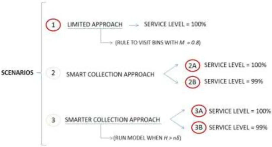
To simulate the installation of sensors inside the waste bins that would provide to the operations manager the actual bins’ fill-level, three scenarios were studied, where the three operational management approaches are applied to Valorsul’s data (see Figure 6). In the first scenario, the limited approach is applied and it is assumed that all bins that surpass the minimum fill-level of 80% of the bins’ capacity must be visited. The second scenario, involves the application of the smart collection approach. Finally, the third scenario consists in the application of the smarter collection approach. For the second and the third scenarios, two different service levels were considered: A) service level equal to 100%, meaning that all bins must be collected before overflowing; and B) service level equal to 99%, meaning that 2 out of 226 bins are allowed to overflow without being collected immediately.
16 The case study data is shown in Table 2. Transportation cost C includes fuel consumption, maintenance of the vehicle and the drivers’ wages. Regarding revenues, the value paid by Sociedade Ponto Verde (the packaging waste regulator in Portugal) for each ton of paper/cardboard collected and sorted by a waste collection company is 136€/ton. This value intends to cover the costs with collection and sorting operations and assumes that the collection operation represents about 70% of the total cost (Ramos et al., 2014). Therefore, since in this work only the collection activity is being considered, the selling price (parameter R) is adjusted to 95.2€/ton (70% x 136€/ton). The penalty for the use of the vehicles (Ω) is set to a small value (0.1€) just to force the model to allocate the least possible number of vehicles. The vehicle capacity Q, in kg, was determined considering the vehicles’ volume (20m3, according to Valorsul
data) and the density of the material inside the vehicle, after being compacted (250kg/m3, again
according to Valorsul data). Paper density inside the waste bins (B) is calculated assuming an average value for the routes performed during the analyzed period of time. Distances dij were
calculated using a Euclidian distance, adjusted by a correction factor (to adjust the straight-line distance to the actual road distance). The correction factor was set to 1.58 according to Silva (2016). The amount of waste at bin i, Si, simulates the values that the sensors will read and
transmit every day. To apply the models, the bins’ fill-levels registered by the team for day 1 and the accumulation rate ai for the following days are considered. The bins’ capacity in kg, Ei, was
calculated multiplying the volume of a bin (2.5 m3) by the density of the paper/cardboard inside
the bins (B=29.5 kg/m3). The total number of bins (n) is equal to 226 and the percentage of bins
which are allowed to overflow (δ) is equal to 0% for scenarios 2.A and 3.A and 1% for scenarios 2.B and 3.B, since the considered service level to be offered is 100% and 99%, respectively. The maximum overflowing threshold (ψ) is equal to 100% of the bins’ capacity for scenarios 2.A and 3.A and 120% of the bins’ capacity for scenarios 2.B and 3.B, since the considered service level to be offered is 100% and 99%, respectively. The number of overflowing bins, H, is calculated summing the number of waste bins for which Si + ai > Ei and can be different for each day the
model is run, depending on the amount of waste at each bin i, Si.
Table 2: Parameters values and sources
Parameters Values Source
C 1€/km Valorsul
R 0.0952€/kg SPV
Ω 0.1€ -
Q 5000kg Valorsul
B 29.5kg/m3 -
dij Adjusted Euclidian distance -
Si Team records for day 1 Valorsul
Ei 75kg Valorsul
n 226 bins Valorsul
δ 0% (for scenarios 2.A and 3.A)
1% (for scenarios 2.B and 3.B) Valorsul
Ψ 100% (for scenarios 2.A and 3.A) 120% (for scenarios 2.B and 3.B) Valorsul
The models were implemented in GAMS 24.6.1and solved with CPLEX Optimizer 12.6.3, on an Intel Xeon CPU X5680 @ 3.33GHz. The CPU time was limited to four hours for each day t.
17 4.1 Scenario 1
Since, in this scenario, the bins to be emptied are selected during the heuristic procedure, it is not possible to consider different service levels. Thus, the considered service level is equal to 100% and there are no bins overflowing. Furthermore, when applying the heuristic procedure, the value of the minimum fill-level (M) above which bins must be visited is assumed to be equal to 80% of the bins’ volume, i.e. every bin which has 80% or more of its total volume filled must be emptied on that day.
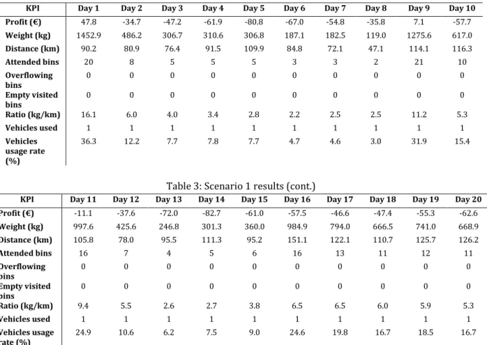
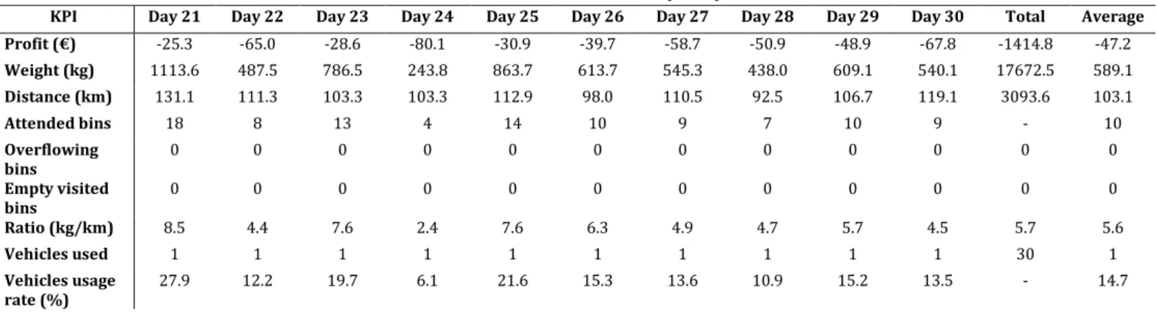
Table 3 shows the results for this scenario. In every day of the period in study (30 days), a single route is performed, even when just 2 or 3 bins must be emptied (e.g. days 6, 7 and 8). Even though no empty bins are visited on those routes, little amount of waste is collected while large distances are travelled, resulting in an inefficient operation. Such inefficiency is shown in Table 3 where very low kg per km ratios are reached and, in most days, negative profit values are obtained. The average rate of vehicles usage is also very low (less than 15%). The maximum number of bins being visited occurs in day 9 (21 attended bins).
Comparing this scenario with the current situation, we can determine that the total distance to be covered in scenario 1 is twice as large (3 093 vs. 1 468 km). This is justified due to the fact that a route is performed every single day and trucks travel large distances to collect fewer bins. Such results motivate the need for having a model capable of choosing the bins that are worth to be visited considering their fill-levels and locations.
Table 3: Scenario 1 results
KPI Day 1 Day 2 Day 3 Day 4 Day 5 Day 6 Day 7 Day 8 Day 9 Day 10
Profit (€) 47.8 -34.7 -47.2 -61.9 -80.8 -67.0 -54.8 -35.8 7.1 -57.7 Weight (kg) 1452.9 486.2 306.7 310.6 306.8 187.1 182.5 119.0 1275.6 617.0 Distance (km) 90.2 80.9 76.4 91.5 109.9 84.8 72.1 47.1 114.1 116.3 Attended bins 20 8 5 5 5 3 3 2 21 10 Overflowing bins 0 0 0 0 0 0 0 0 0 0 Empty visited bins 0 0 0 0 0 0 0 0 0 0 Ratio (kg/km) 16.1 6.0 4.0 3.4 2.8 2.2 2.5 2.5 11.2 5.3 Vehicles used 1 1 1 1 1 1 1 1 1 1 Vehicles usage rate (%) 36.3 12.2 7.7 7.8 7.7 4.7 4.6 3.0 31.9 15.4
Table 3: Scenario 1 results (cont.)
KPI Day 11 Day 12 Day 13 Day 14 Day 15 Day 16 Day 17 Day 18 Day 19 Day 20
Profit (€) -11.1 -37.6 -72.0 -82.7 -61.0 -57.5 -46.6 -47.4 -55.3 -62.6 Weight (kg) 997.6 425.6 246.8 301.3 360.0 984.9 794.0 666.5 741.0 668.9 Distance (km) 105.8 78.0 95.5 111.3 95.2 151.1 122.1 110.7 125.7 126.2 Attended bins 16 7 4 5 6 16 13 11 12 11 Overflowing bins 0 0 0 0 0 0 0 0 0 0 Empty visited bins 0 0 0 0 0 0 0 0 0 0 Ratio (kg/km) 9.4 5.5 2.6 2.7 3.8 6.5 6.5 6.0 5.9 5.3 Vehicles used 1 1 1 1 1 1 1 1 1 1 Vehicles usage rate (%) 24.9 10.6 6.2 7.5 9.0 24.6 19.8 16.7 18.5 16.7
18
Table 3: Scenario 1 results (cont.)
KPI Day 21 Day 22 Day 23 Day 24 Day 25 Day 26 Day 27 Day 28 Day 29 Day 30 Total Average
Profit (€) -25.3 -65.0 -28.6 -80.1 -30.9 -39.7 -58.7 -50.9 -48.9 -67.8 -1414.8 -47.2 Weight (kg) 1113.6 487.5 786.5 243.8 863.7 613.7 545.3 438.0 609.1 540.1 17672.5 589.1 Distance (km) 131.1 111.3 103.3 103.3 112.9 98.0 110.5 92.5 106.7 119.1 3093.6 103.1 Attended bins 18 8 13 4 14 10 9 7 10 9 - 10 Overflowing bins 0 0 0 0 0 0 0 0 0 0 0 0 Empty visited bins 0 0 0 0 0 0 0 0 0 0 0 0 Ratio (kg/km) 8.5 4.4 7.6 2.4 7.6 6.3 4.9 4.7 5.7 4.5 5.7 5.6 Vehicles used 1 1 1 1 1 1 1 1 1 1 30 1 Vehicles usage rate (%) 27.9 12.2 19.7 6.1 21.6 15.3 13.6 10.9 15.2 13.5 - 14.7 4.2 Scenario 2
In this scenario, the optimization model for the Smart Waste Collection Routing Problem is solved for every day of the 30-day period. The bins to be visited, as well as the optimal sequence of collection are obtained.
Tables 4 and 5 show the results for scenario 2. For a service level of 100% (Table 4), a collection route must be performed almost every 2-3 days during the time horizon and there are no overflowing bins due to the service level of 100%. In this scenario, the model is in fact able to choose the best bins to visit. Since the model is run every day, it selects the set of bins that will maximize the profit for that particular day and does not take the following days into consideration.
Table 4: Scenario 2.A results
KPI Day 1 Day 4 Day 7 Day 11 Day 14 Day 15
Profit (€) 212.1 13.1 43.5 59.6 45.8 -49.1
Weight (kg) 4422.5 1215.4 2405.2 2438.7 2063.6 910.5
Distance (km) 208.0 102.3 185.0 172.1 150.3 135.6
Attended bins 106 101 152 142 121 90
Overflowing bins 0 0 0 0 0 0
Empty visited bins 0 0 0 0 0 0
Ratio (kg/km) 21.3 11.9 13.0 14.2 13.7 6.7
Vehicles used 2 1 1 1 1 1
Vehicles usage rate (%) 55.3 30.4 60.1 61.0 51.6 22.8
Table 4: Scenario 2.A results (cont.)
KPI Day 17 Day 19 Day 20 Day 23 Day 26 Day 29 Total Average
Profit (€) 10.4 28.7 -80.9 77.6 25.5 36.0 422.4 35.2
Weight (kg) 661.9 1932.8 347.4 3037.9 1368.9 1785.8 22590.4 1882.5
Distance (km) 52.5 155.0 113.9 210.9 104.5 133.6 1723.7 143.6
Attended bins 45 125 44 168 104 122 - 110
Overflowing bins 0 0 0 0 0 0 0 0
Empty visited bins 0 0 0 0 0 0 0 0
Ratio (kg/km) 12.6 12.5 3.0 14.4 13.1 13.4 13.1 12.5
Vehicles used 1 1 1 1 1 1 13 1
19 For a service level of 99% (Table 5), corresponding to a maximum of two bins in overflow, this is only observed in day 22, as in the other days there is one or no bins overflowing. Compared to a service level equal to 100%, fewer routes are required (11 routes vs. 13 routes) and, in general, the results are better. In scenario 2B, the total profit is higher than in scenario 2A (548€ vs. 422€), and the same is observed for: the total kg per km ratio (14 vs. 13); vehicles usage average rate (50 vs. 42%); and the total distance travelled, in this case is shorter than in scenario 2A (1 568 vs. 1 724 km). For both service levels, the only day when two trucks are needed is in day 1, when the kg per km ratio is significantly bigger than the average.
When comparing these results with the current situation, these are however generally worse: scenario 2 represents smaller amounts of total waste being collected (22 590 (2A) and 22 272 (2B) vs. 22 692 kg) and higher total distances being travelled (1 724 (2A) and 1 568 (2B) vs. 1 468 km), besides a smaller total kg per km ratio (13 (2A) and 14 (2B) vs. 15) and smaller vehicles usage average rates (42 (2A) and 50 (2B) vs. 57%). This fact justifies the development of scenario 3, where the selection of the best days to perform the routes during the time horizon is at stake.
Table 5: Scenario 2.B results
KPI Day 1 Day 4 Day 7 Day 10 Day 13 Day 16 Day 19 Day 22 Day 25 Day 28 Total Average
Profit (€) 212.1 13.1 49.4 27.5 52.7 26.5 49.3 27.5 66.4 23.3 548.0 54.8 Weight (kg) 4422.5 1215.4 2543.0 1388.9 2761.6 1358.5 2657.0 1336.0 3291.6 1297.1 22271.7 2227.2 Distance (km) 208.0 102.3 192.1 104.4 209.6 102.6 203.1 99.4 246.3 99.9 1567.8 156.8 Attended bins 106 101 156 104 163 101 161 98 179 99 - 127 Overflowing bins 0 0 0 0 0 1 1 2 1 0 5 0.5 Empty visited bins 0 0 0 0 0 0 0 0 0 0 0 0 Ratio (kg/km) 21.3 11.9 13.2 13.3 13.2 13.2 13.1 13.4 13.4 13.0 14.2 13.9 Vehicles used 2 1 1 1 1 1 1 1 1 1 11 1 Vehicles usage rate (%) 55.3 30.4 63.6 34.7 69.0 34.0 66.4 33.4 82.3 32.4 - 50.1 4.3 Scenario 3
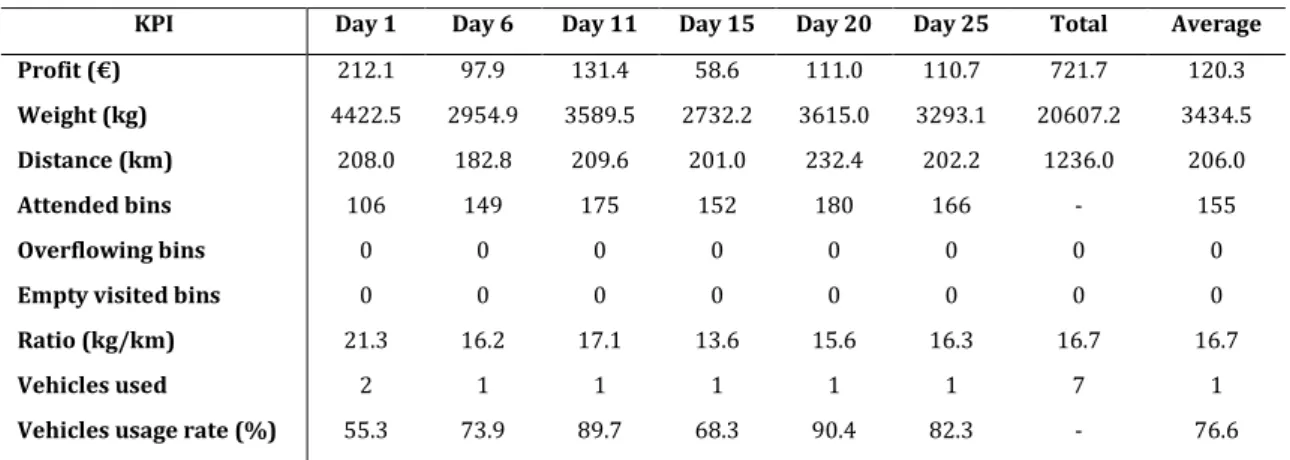
Finally, when applying the third operational management approach which combines a heuristic procedure to define the best days to perform a route through the Smart Waste Collection Routing model, fewer routes are defined and a more efficient vehicle usage rate is obtained, as shown in Tables 6 and 7. For a service level equal to 100%, only 7 routes are performed in 6 days, and for a 99% service level, 8 routes are defined in only 4 days.
Table 6: Scenario 3.A results
KPI Day 1 Day 6 Day 11 Day 15 Day 20 Day 25 Total Average
Profit (€) 212.1 97.9 131.4 58.6 111.0 110.7 721.7 120.3
Weight (kg) 4422.5 2954.9 3589.5 2732.2 3615.0 3293.1 20607.2 3434.5
Distance (km) 208.0 182.8 209.6 201.0 232.4 202.2 1236.0 206.0
Attended bins 106 149 175 152 180 166 - 155
Overflowing bins 0 0 0 0 0 0 0 0
Empty visited bins 0 0 0 0 0 0 0 0
Ratio (kg/km) 21.3 16.2 17.1 13.6 15.6 16.3 16.7 16.7
Vehicles used 2 1 1 1 1 1 7 1
20
Table 7: Scenario 3.B results
KPI Day 1 Day 8 Day 15 Day 21 Total Average
Profit (€) 212.1 190.2 196.7 138.6 737.6 184.4
Weight (kg) 4422.5 4606.3 4797.4 4250.4 18076.6 4519.1
Distance (km) 208.0 247.3 259.1 265.2 979.7 244.9
Attended bins 106 185 186 184 - 165
Overflowing bins 0 1 1 2 4 1
Empty visited bins 0 0 0 0 0 0
Ratio (kg/km) 21.3 18.6 18.5 16.0 18.4 18.6
Vehicles used 2 2 2 2 8 2
Vehicles usage rate (%) 55.3 57.6 60.0 53.1 - 56.5
Moreover, as the real situation corresponds to a service level of 99%, for the same service level (scenario 3B) this approach finds a solution that globally increases both the kg per km ratio (from 15 kg/km to 18 kg/km), as well as the total profit (from 687€ to 738€) significantly, meaning that more waste has been collected with less distance travelled (from 1468 km to 980 km). Unlike the current real case, where more than 80 empty bins were visited in the period, in this scenario there are no empty visited bins. Additionally, and just as in scenario 2B, no bin exceeds the maximum overflowing threshold, i.e., all the overflowing bins are emptied before they reach 120% of the bins’ capacity. As an example, at day 8, the bin number 24 is registered to be overflowing (fill-level =109% of the bins’ capacity), but it is emptied at the same day; the same happens at days 15 and 21; in this last day, bins 24 (fill-level =109%) and 364 (fill-level = 104%) are overflowing and both are emptied.
The model allocates two vehicles each day a route is performed meaning that the bins were fuller than in the other scenarios (there was more waste available to be collected). Besides this fact, the number of total vehicles required for the collection decreases when compared to the real situation (from 10 to 8 vehicles), representing significant savings for Valorsul and a reduction of emissions of pollutant gases.
Analyzing in detail some of the results obtained for scenario 3, an interesting situation is observed. For a service level equal to 99%, and in day 8, for example, when defining the routes the model decides to collect bins that are not full. This is because the route passes near such bins and the revenues of collecting them surpasses the costs of doing so. This situation is depicted in Figure 5 where it is possible to see the two routes performed in day 8, where bin 103 is collected, in red (with a fill-level of 20%). From Figure 5 it can also be seen that bin 359, in blue, is an example of a bin that is almost full (fill-level of 75%) but was not collected as it was not near enough to be worth to visit. Figure 7 also shows that the route defined for day 8 includes bins from the three pre-defined routes (route 6, 11 and 13).
21
Figure 7: Collection routes of day 8 (Scenario 3.B)
4.4 Summarized scenarios comparison
As global conclusions, Figure 8 shows, for all scenarios analyzed, the values obtained for the key performance indicators: kg per km ratio; profit; distance travelled; and vehicle usage rate. Considering the service level of 99% that represents Valorsul’s actual operation (“blind collection”), it is possible to see that exploring the presence of sensors in the bins coupled with the operational management approach described in scenario 3 (which was proved to be the best alternative operational management approach), an improvement of 20% on the kg per km ratio is observed, as well as 7% profit increase (Current Solution vs. Scenario 3.B), while the distance travelled decreases in 33%. These improvements are due to an increase in the amount of waste collected (since the bins are collected as late as possible, and thus the waste can accumulate in some bins), while at the same time, empty bins are not visited. It is important to note that this happens in all studied scenarios and thus no resources are spent to visit empty bins. However, if Valorsul aims to increase the service level to 100%, there is a need to perform more routes and this reduces the kg per km ratio and the profit while increases the distance travelled by 26% when compared to the value registered for the 99% service level (Scenario 3.B vs. Scenario 3.A). Nevertheless, this case also shows better key performance indicators when compared to the current situation (Scenario 3.A vs. Current situation).
22
Figure 8: Comparison of some key performance indicators for the current situation and the three scenarios studied.
5. Conclusions
This work introduces the Smart Waste Collection Routing Problem, where it is assumed that uncertainty regarding the amount of waste in each bin is reduced by installing sensors capable of reading and transmitting the bins’ fill-levels in real-time. This allows the definition of dynamic routes to collect only the more attractive bins resulting in an improvement of the operations´ efficiency.
Three different operational management approaches are studied to deal with the information transmitted by the sensors: 1) a limited approach, in which a minimum fill-level rule is imposed; 2) a smart collection approach, that uses a model to decide the best bins and the best sequence to collect them; and 3) a smarter collection approach, that uses a combination of a heuristic method to decide the best days to collect the bins, with the smart collection model developed in approach 2). To validate the three approaches, data from a real case-study was used and for each approach, the impacts on profit, distance travelled, kg per km ratio and vehicle usage rate were assessed and compared to the company’s current operation. The results show that the third operational management approach is the most efficient of the three, leading to a potential company’s profit increase of 7%, which represents a meaningful managerial insight for practical implementations. From this work major findings are established: a model able to choose the bins to be visited considering their fill-levels and their location leads to higher values of profit and less pollutant
23 gases emissions when compared to a situation where the model is just used to optimize a pre-defined selection of bins; knowing the amount of waste at each bin does not necessarily means that only full containers should be collected on a specific day - the model is able to consider that minimizing the distance might not be the most efficient solution in terms of resources usage as small additional distances may reveal more profitable situations (e.g. collecting less than full containers located nearby a full container). Additionally, defining the more “profitable” route for a day does not mean that the profit will be maximized for a time horizon (as a decision in one day often has repercussions on the following days, and thus longer planned time horizons should be considered). Based on these findings, it can be concluded that the Smarter Waste Collection approach is efficient in improving waste collection operational systems and is generic enough to be applied to other recyclable materials.
As for future work, three main ideas can still be explored. Firstly, the solution approach could be applied to a larger time horizon exploring a tactical level of planning, allowing in this way a better planning of resources. In this sense, the expected daily accumulation rate (ai) could be used to
simulate the bins’ fill-levels permitting a broader planning assisting decision making in the medium and long term. Secondly, as the success of the Smart Waste Collection model concerns the reduction on the uncertainty associated with the fill-levels, and this still may exist on the sensors’ information, a sensitivity analysis could be a first step to address such concern. However, the development of stochastic or robust optimization approaches should be the path to follow. These approaches could also be extended to address other types of uncertainties as, for instance, cost factors. Thirdly, as the sensors investment can be very high, an interesting extension of the current problem would be the development of a model to decide which containers should be monitored considering the costs involved.
Acknowledgements
This work was supported by the Smart2 Project – Smart Cities & Smart Grids for Sustainable
Development, as a partnership of the Erasmus Mundus Programme [Application number SS15DF0179], and by the financial support of “Fundação para a Ciência e Tecnologia” (FCT – Portugal), through the research project MIT-EXPL/SUS/0132/2017.
References
Aksen, D., Kaya, O., Salman, F. S. and Akça, Y., 2012. Selective and periodic inventory routing problem for waste vegetable oil collection. Optimization Letters, Vol. 6, p. 1063 - 1080.
Anagnostopoulos, T., Kolomvatsos, K., Anagnostopoulos, C., Zaslavsky, A. and Hadjiefthymiades, S., 2015. Assessing dynamic models for high-priority waste collection in Smart Cities. Journal of Systems and Software, Vol. 110, p. 178-192.
Anghinolfi, D., Paolucci, M., Robba, M. and Taramasso, A. C., 2013. A dynamic optimization model for solid waste recycling. Waste Management, Vol. 33, p. 287 - 296.
Apaydin, O., Gonullu, M., 2007. Route optimization for solid waste collection: Trabzon (Turkey) case study. Global NEST J., Vol. 9, p. 6 - 11.
24 Aras, N., Aksen, D. and Tekin, M. T., 2011. Selective Multi-Depot Vehicle Routing Problem with pricing. Transportation Research Part C: Emerging Technologies, Vol. 19, p. 866 - 884.
Archetti, C., Speranza, M. G. and Vigo, D., 2014. Chapter 10: Vehicle routing problems with profits. Vehicle routing: problems, methods, and applications, 2nd edition, Society for Industrial and Applied Mathematics, Philadelphia.
Atzori, L., Iera, A., Morabito, G., 2017. Understanding the Internet of Things: definition, potentials, and societal role of a fast evolving paradigm. Ad Hoc Networks, vol. 56, p. 122 - 140.
Baldacci, R., Hadjiconstantinou, E. and Mingozzi, A., 2004. An exact algorithm for the Capacitated Vehicle Routing Problem based on a two-commodity network flow formulation. Operations research, vol. 52, p. 723 - 738.
Belien, J., De Boeck, L. and Van Ackere, J., 2012. Municipal Solid Waste Collection and Management Problems: A Literature Review. Transportation Science, Vol. 48, p. 1 - 40.
Daugherty, P. J., Richey, R. G., Genchev, S. E. and Chen, H., 2005. Reverse logistics: superior performance through focused resource commitments to information technology. Transportation Research Part E, vol. 41, p. 77 - 92.
EUROSTAT – Statistics Explained (2017). Waste statistics. Available at: http://ec.europa.eu/eurostat/statistics-explained/index.php/Waste_statistics
Faccio, M., Persona, A., Zanin, G., 2011. Waste collection multi objective model with real time traceability data. Waste Management, Vol. 31, p. 2391 - 2405.
Fayoumi, A. and Loucopoulos, P., 2016. Conceptual modeling for the design of intelligent and emergent information systems. Expert Systems with Applications, Vol. 59, p. 174 - 194.
Gonçalves, D. S. Tecnologias de informação e comunicação para otimização da recolha de resíduos recicláveis. Master’s thesis, Lisboa: ISCTE-IUL, 2014.
Ghiani, G., Laganà, D., Manni, E., Musmanno, R. and Vigo, D., 2014. Operations research in solid waste management: A survey of strategic and tactical issues. Computers & Operations Research, Vol. 44, p. 22 - 32.
Gruler, A., Quintero-Araújo, C. L., Calvet, L. and Juan, A. A., 2017. Waste collection under uncertainty: a simheuristic based on variable neighbourhood search. European Journal of Industrial Engineering, vol. 11, no. 2, p. 228 - 255.
Gutierrez, J. M., Jensen, M., Henius, M and Riaz, T., 2015. Smart waste collection system based on location intelligence. Procedia Computer Science, vol. 61, p. 120-127.
Han, H. and Ponce-Cueto, E., 2015. Waste Collection Vehicle Routing Problem: Literature Review. Traffic & Transportation, Vol. 27(4), p. 345 - 358.
Hannan, M.A., Mamun, M.A.A., Hussain, A., Basri, H., Begun, R.A., 2015. A review on technologies and their usage in solid waste monitoring and management systems: Issues and challenges. Waste Management, Vol.43, p. 509-523.