A Work Project, presented as part of the requirements for the Award of a Master Degree in Finance from the NOVA – School of Business and Economics.
ACTIVE PORTFOLIO MANAGEMENT USING THE
BLACK-LITTERMAN MODEL
Catarina Muacho Anacleto 2452 José Valadas 2411
Theresa Felder 2448
A Project carried out on the Master in Finance Program, under the supervision of Martijn Boons from Nova SBE and Pedro Frada and Paulo Ribeiro from Caixagest
Abstract
In this project, we are studying the application of the Black-Litterman model for active portfolio management. We focus on three elements that are important for a real-world application of the model. First, we present a robust construction of the variance-covariance matrix that is used as input for the model. Second, we present a rigorous explanation of the model as it was presented initially by Black and Litterman, which is important to highlight the driving mechanisms inside the model. Third, we describe how to adjust the model to an application in an active setting, where the investor is evaluated relative to a benchmark. Empirical evidence for the active case is limited to date. Working with a range of benchmarks (relevant for various types of investors), we derive a portfolio that includes multiple asset classes and present the results obtained under the application of the model. Finally, a simulation exercise was developed to understand how the model reacts to its inputs.
3 Contents 1. Introduction ... 4 2. Theoretical context ... 6 3. Literature review ... 7 4. Data ... 12 4.1. Data treatment. ... 12
4.2. Returns and descriptive statistics ... 16
5. The Variance-Covariance Matrix: An input to the Black-Litterman model …. 17 5.1. The importance of the covariance Matrix ………. 17
5.2. Methods of estimation of the Covariance matrix ……….. 18
5.2.1. Historical Method ……… 18
5.2.2. The exponentially weighted moving average ……….. 20
5.2.3. GARCH... 22
5.3. Invertibility ... 24
5.4. Analysis of the Covariance estimations ………. 25
5.4.1. Non-overlapping analyses of the estimations ……….. 26
5.4.2. Overlapping analyses of the estimations ……….. 27
6. The Black-Litterman model ………... 29
6.1. Limitations of the Markowitz Optimization – An introduction to the Black-Litterman Framework ……….. 29 6.2. Overview ... 31
6.3. Equilibrium Returns ... 32
6.4. The Black Litterman formula ... 35
6.5. Investors’ Views: P, Q and Ω Matrix ………. 36
6.6. BL excess returns and optimal weights ……….. 40
6.7. Caixagest portfolio – Initial Black Litterman model ………. 41
6.7.1. Simulation and Model Analysis ………... 43
7. Black Litterman and Active Management... 48
7.1. Black Litterman framework ... 48
7.2. Formulation of the new model... 49
7.3. Problems of applying Black-Litterman in active management ……….. 52
7.4. Black-Litterman model and Active Management ……….. 55
7.5. Solution: New vector of excess returns ... 55
7.6. Implementation- General case ... 57
7.7. Qualitative views ... 53
7.8. Constraints added to the initial setting ... 59
7.9. Risk Analysis... 59
7.10. CaixaGest portfolio - Active Management ... 63
7.10.1. Risk analysis ... 67
7.10.2. Simulation ... 69
8. Conclusion ... 77
Section 1. Introduction
How to allocate one’s wealth in a variety of assets and portfolio optimization are topics widely discussed in literature and crucial for investment banks. The major drawback of the Markowitz optimization (developed in 1952) is that it can lead to corner solutions, which is highly undesirable for portfolio managers. They develop accurate estimations of expected returns to aim for a more diversified portfolio. Thus, this optimization method is not often used in practice. Black and Litterman (1992) introduced the Black-Litterman (BL) asset allocation model, which has the advantage of considering the forward-looking investor’s views for the estimation of the expected excess returns. The views are investors’ opinions on how the market or specific assets will perform in the future. In addition to the opinions regarding the market, investors need to specify their confidence about them; this confidence level will be vital to understand how much the final portfolio weights will tilt away from the market portfolio. All in all, the main idea of this model is to start the portfolio construction with a neutral reference point which is the market equilibrium, that will then suffer deviations due to the specific investors’ views and their respective confidence. Black and Litterman argue that their model leads to a more diversified portfolio.
However, applying this model in the active portfolio management, where one evaluates the weights’ deviations relative to a given benchmark portfolio, comes along with some problems. The initial BL model aims to maximize the Sharpe ratio of a portfolio-average return earned in excess of the risk-free rate per unit of volatility or total risk. On the contrary, under an active management environment, it is the investor’s intention to maximize the information ratio, which involves to maximize the portfolio’s alpha (active return) per unit of tracking error. As a result, if the benchmark portfolio is not chosen to be the Global Minimum Variance portfolio, the portfolio will move away from the benchmark even if no views are specified. This is due to the mismatch of the defined objective functions defined in the original BL model and in the
5 active management framework, that leads the investor to believe that he/she can take advantage of alpha opportunities that in fact do not exist.
The goal of the project is to implement the BL framework in a portfolio of indexes given by Caixagest with a major focus on the active portfolio management. Caixagest is the asset management subsidiary of the group Caixa General Depósitos (CGD) and is specialized in the mutual fund management and portfolio fund management, having a huge portfolio of different funds diversified by global financial markets. In this Work Project, we present several ways of implementing the model under analysis always followed by an explanation of the results based on portfolio statistics. In the end, Caixagest should have an essential basis for deciding if this asset allocation method is an appropriate one to suggest to its investors and under which hypothesis it wants to work with. Moreover, Caixagest should be able to apply the BL model for every type of investor as, in the active framework, different benchmarks that mirror different risk appetites (defensive, balanced and dynamic) are considered. It is crucial for Caixagest to understand how the views impact the different risk profiles in the active management framework, so that they can give the most accurate advice to each type of investor.
It is important to mention that this project is supported and has it basis in many academic papers, which constituted a great help in order to implement the model in the portfolio of indexes that we are working with. In a first step, this paper focus on the estimation methods of the variance-covariance matrix since this is an important input of the BL model and in portfolio theory in general. Second, we introduce the initial BL model as it was developed by Black and Litterman with a detailed explanation of all it inputs. Moreover, we implement the BL model for an active portfolio management environment. An exhausting analysis of the results implying the BL method is followed. Our Work Project also introduces a simulation exercise in which the goal is to understand how the model, particularly the weights allocation, reacts when the inputs change and some constraints are added to the initial setting. In this simulation, we focused on
the analysis of the reaction of the active and, consequently, portfolio weights to different types of returns- the first ones result from the implementation of the initial BL framework and the second ones from considering the active reformulation of the BL returns. Which model is better to work with and gives more accurate results when compared with the initial unconstrained BL framework is not trivial, in the sense that both cases have pros and cons. One can point out that using the initial BL returns leads to a higher active return for the types of investor analysed. However, when considering the more constrained portfolio, the correlation between the active weights and the returns of the assets included in the views is negative, which goes against the fact that if an investor specifies a positive view in a certain asset, the correspondent active weight should move in the same direction. On the other hand, a positive correlation between the weights previously mentioned is positive when one considers the reformulation of the returns that will be presented in the BL framework. Furthermore, it is important to notice that when doing a comparison between the final weights of the portfolio and the tangency, the correlation is higher when one considers the initial BL returns, which allows to have a notion of if the portfolio obtained is moving towards the tangency.
We conclude our report with further research suggestions.
Section 2. Theoretical context
As referred in section 1, the aim of this project is to apply the active BL model to a real portfolio of assets that was given to us by the company. In order to fulfill this purpose, we closely followed the work that was performed by some investment banks that are already using the model to allocate weights to the assets included in a portfolio. The project was also supported and has it basis in many academic papers that study, for instance, the implications, advantages and disadvantages of using this model under active management. This project came associated
7 with some business challenges in the sense that we needed to adapt the initial model developed by Black and Litterman in the early 1990s for the type of Caixagest’s investors and to its investment strategy. Thus, the main goal of using this model was to obtain a more diversified portfolio with not much concentration in just a few assets, allowing to a higher diversification of risk. As a result, we needed to reformulate the original framework in which the model was built and to study the inclusion of some constraints on it, such as a risk target per type of investor or account for the fact that no short selling is allowed. Finally, another challenge that we needed to face was based on the difficulty of building some of the inputs needed to implement the model, an issue discussed in existing literatures.
Section 3. Literature review
Starting by the estimation of the variance-covariance matrix, our project has as support and is closely related with some papers that analyse the difference between the diverse methods that can be used in order to obtain a robust estimation of this important input to the BL model. Furthermore, some papers that specifically discuss the three methods that will be studied and implemented in this project were also considered, namely the historical method, the Exponentially Weighted Moving Average (EWMA) and the Generalized Auto Regressive Conditional Heteroskedasticity (GARCH) method.
Some basic properties of covariances, variances and correlations are described by Carol Alexander (2007). He presents the different methods of calculating variances and covariances, namely the EWMA and the equally weighted average methods, explaining all the different inputs that each model requires; the GARCH model is briefly mentioned as well. In the paper, he argues about the forecast (predictive) power of each model and presents the advantages and drawbacks of each one. The criticisms go mainly to the historical formula, also called the
equally weighted average method, which is presented with many pitfalls, such as the fact that extreme events are just as important to current estimates whether they occurred yesterday or very far in the past. All in all, the paper suggests that the historical method is obsolete and is not appropriate anymore to model volatility, since other methods such as the EWMA and the GARCH method are available.
Laplante, Desrochers and Préfontaine (2008) provide research not only on the GARCH model but also on other methods that serve as risk predictors in financial applications. The authors put forward the importance of having good estimates of the variances and covariances for financial portfolios: according to them, using forecasts that do not provide a reasonable estimate of variances and covariances close to their actual value can result in a wrong portfolio mix. In the paper, they first examine and compare three different variance and covariance estimation methods, namely the JP Morgan’s EWMA, the historical mean, the random walk and a GARCH (1,1). Then, the authors analyse and measure the effectiveness of all methods in forecasting the standard deviation of a minimum variance portfolio using several econometric statistics, such as the root-mean square error, mean absolute error and mean absolute percentage error. Their results provide confirmatory evidence that both the GARCH (1,1) and the EWMA preform way better than the historical estimate. Their findings also suggest that the GARCH is the best method to estimate the variances and covariances as all the indicators computed based on this model are the lowest ones. These results were supported by many authors, such as Brailsford and Faff (1996) and West and Cho (1997). Nevertheless, Alexander and Leigh (1997) studied three models in order to forecast the covariance matrix, and concluded that the EWMA preforms better than the GARCH model. Thus, the literature shows no consensus on which method to systematically use to model volatilities.
When one mentions the GARCH model, it is important to refer to Engle (2001) who is prominent in the literature on modelling variances for financial applications. His paper focuses
9 on the Autoregressive Conditional Heteroskedasticity (ARCH) and GARCH models. The need to use a GARCH model comes from the presence of a “volatility clustering” and high degree of autocorrelation in the “riskiness of financial returns”. In the paper, all the inputs of the GARCH are described when modelling the variance and the implementation of a GARCH (1,1) is explained as well. The author encouraged other ones as Bollerslev (1986), who only focuses on the GARCH model and goes beyond a simple explanation of the model by developing it in detail. The author finally gives an empirical example, related to inflation rate uncertainty, very helpful to fully understand the dynamics of the GARCH model. As one can see, there is ample support for the claim that a GARCH (1,1) is very capable to model volatility.
It is very important to have a robust variance covariance matrix to input in the BL model, which is an asset allocation method used to overcome the problem of unintuitive, highly-concentrated and input-sensitive portfolios. Input sensitivity is a well-documented problem with mean-variance optimization and is the most likely reason that more portfolio managers do not use the Markowitz optimization, in which return is maximized for a given level of risk.
In addition to describing the intuition behind the BL Model, the paper of Idzorek (2005) consolidates critical insights contained in the various works on the BL model and focuses on the details of actually combining market equilibrium expected returns with “investor views” to generate a new vector of expected returns. At this time, relative few works on the model were published and thus, the aim was to provide instructions by describing the model and the process of building the required inputs in very detail, which enables the reader to implement this complex model. Furthermore, a new method for determining Ω was introduced: it allows the specification of the investor view confidence as a percentage, where the model will back out the proper value of Ω to reach the confidence level specified.
In their paper, Benzschawel and Su (2015) focus mainly on asset allocation across major fixed income sectors. The paper points out the major shortcomings of mean-variance optimization
and thus, explains the benefits of extending vesting duration, investing in a diversified portfolio of asset classes, and optimization methods. The authors explain deeply the mean-variance optimization because it comprises the final stage of the BL model. Furthermore, they allocate a great part of the paper to the description of the inputs used in the model and various equivalent formulations and their implications. Besides the focus on the mechanics of inputting views into the model and controlling the relationship between investors’ views and market returns, the authors provide a step-by-step formulation of the model, resolve ambiguities and use examples to demonstrate the effects of parameter choices on resulting optimizations. Finally, they compare performance of model-based estimates of sector returns, the effects of risk and equilibrium parameters and how investors’ view uncertainty affects allocations.
Walters (2014) focus on the canonical model including full derivations from the underlying principles using both Theil's Mixed Estimation model and Bayes Theory and a full description of this model. The author describes the fact that the BL model uses a Bayesian approach to combine the investor’s views with the market equilibrium vector of expected returns to form a new, mixed estimate of expected returns. He also describes the theory behind the BL model and its inputs including all the various formulas.
Since its publication in 1990, the BL asset allocation model has gained wide application in many financial institutions as it provides the flexibility to combine the market equilibrium with additional market views provided by the investor. Thus, the user inputs any number of views and statements about the expected returns of arbitrary portfolios, and the model combines those views with equilibrium, producing a set of expected returns for the assets that are included in the portfolio and the resulting portfolio weights. As the investors usually want to beat a specific benchmark, the initial model was also extended to an active setting by some practitioners. In the article developed by the Goldman Sachs’ Investment Management Research Team, He and Litterman (1999) present examples to illustrate the difference between the traditional
mean-11 variance optimization process (which can produce results that are extreme and not intuitive) and the BL one. Moreover, they show that the optimal portfolios that result from the BL framework have intuitive properties, such as the fact that the unconstrained optimal portfolio is the market equilibrium portfolio plus a weighted sum of portfolios representing an investor’s views. In addition, the weight on a portfolio representing a view is positive when the view is more bullish than the one implied by the equilibrium and other views, being this weight higher as the investor becomes more bullish and confident in the view. This article is also meaningful in the sense that it tests the inclusion of constraints in the optimal portfolio: a risk constraint (the investor aims to maximize the expected return while keeping the volatility of the portfolio under a given level), a budget constraint (forcing the sum of the total portfolio weights to be one) and a beta constraint (forces the beta of the portfolio with respect to the market portfolio to be one).
In the original BL paper, the asset universe to be optimized was constituted of equity in a framework that did not include active management. However, it can be extended to a wider class of assets and to an active management setting; that is what Maggiar (2009) studies in his thesis. Thus, he focusses on the study of the application of the BL model to an active fixed-income portfolio1 management. Maggiar presents a derivation of the model in a general setting and then moves on to apply it to active management, in which one desires to maximize the return of a portfolio with respect to a benchmark. Furthermore, this paper discusses the advantages of the BL model as being a great tool in allocating the portfolio’s weights and an improvement over the classical mean-variance optimization process developed by Markowitz. In particular, Maggiar points out that the highest advantages of this model are the fact that it allocates risk according to the managers’ confidence in their views and offers a great flexibility in the way in which they can be expressed. However, despite its many qualities and advantages
over the allocation methods, the model still suffers from some constraints, namely the assumptions on the distribution of the returns, the parameters that one needs to specify and the imposed linearity of the expression of the views are all factors which limit its optimal use. Maggiar also discusses one of the crucial points of the BL model- the covariance matrix, as previously mentioned- by presenting a “state-dependent model to try to more accurately capture the expected covariance matrix”. Finally, this paper adds to the previous literature the introduction of some risk management tools to assess the benefits of using the BL model in an active management setting, by adapting the method developed by Fusai and Meucci (2003). Moreover, Silva, Lee and Pornrojnangkool (2009) give special attention to the fact that the straight application of the BL framework in active investment management can lead to unintended trades and risk taking, which leads to a riskier portfolio than desired. Thus, focusing on the mismatch between the Sharpe ratio (SR) optimization used in the initial BL framework and the information ratio (IR) optimization that constitutes the goal of the active management, they propose a solution to fix this problem that leads to portable alpha implementation of active portfolios. These resulting active portfolios reflect the real investment insights given by the investors. Furthermore, after explaining the pitfalls of the traditional Minimum-Variance optimization and providing a review of the BL framework, both theoretical and empirical results are provided in order to show how one can go from the original BL setting to the one that includes active management.
Section 4. Data 4.1. Data treatment
At the very beginning, Caixagest team gave us a broad list of assets (Indices divided by asset class) that are used on clients’ portfolio allocation and were previously used by the Caixagest
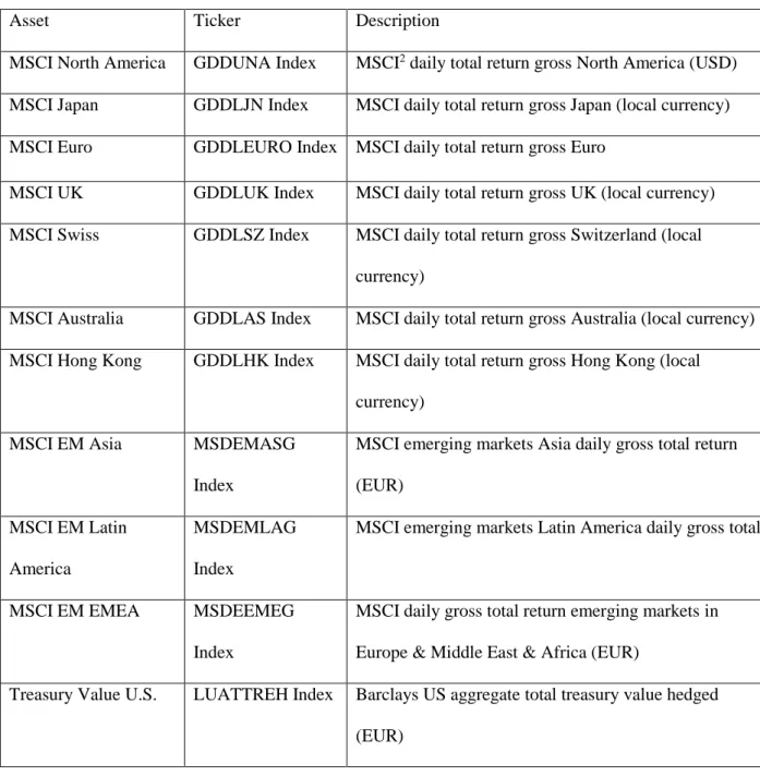
13 team to perform some studies on the BL model. This broad list of assets includes US stock indices, international indices, fixed income instruments from all over the world and an index that tracks commodities price evolution. The list assets whose allocations we are studying in this project are displayed in the following figure:
Figure 1: Assets included in the portfolio and respective description
Asset Ticker Description
MSCI North America GDDUNA Index MSCI2 daily total return gross North America (USD) MSCI Japan GDDLJN Index MSCI daily total return gross Japan (local currency) MSCI Euro GDDLEURO Index MSCI daily total return gross Euro
MSCI UK GDDLUK Index MSCI daily total return gross UK (local currency) MSCI Swiss GDDLSZ Index MSCI daily total return gross Switzerland (local
currency)
MSCI Australia GDDLAS Index MSCI daily total return gross Australia (local currency) MSCI Hong Kong GDDLHK Index MSCI daily total return gross Hong Kong (local
currency)
MSCI EM Asia MSDEMASG
Index
MSCI emerging markets Asia daily gross total return (EUR)
MSCI EM Latin America
MSDEMLAG Index
MSCI emerging markets Latin America daily gross total
MSCI EM EMEA MSDEEMEG
Index
MSCI daily gross total return emerging markets in Europe & Middle East & Africa (EUR)
Treasury Value U.S. LUATTREH Index Barclays US aggregate total treasury value hedged (EUR)
2A MSCI index is a measurement of stock market performance in a particular area. It tracks the
performance of the stocks included in the index. MSCI stands for Morgan Stanley Capital International
Corporate investment U.S.
LUACTREH Index The corporate bond index measures the investment grade fixed rate and taxable corporate bond market; it includes USD denominated securities publicly issued by US and Non-US industrial
JPM Euro JNEUI1R3 Index European sovereign debt up to 3 years (short maturities) Euro-Aggregate
Treasury
LEATTREU Index Barclays euro treasury index an index that contains 13 Euro countries (all maturities)
Euro-floating rate LEF1TREU Index Benchmark that measures the investment grade, fixed rate bond market, including treasuries, governments (EUR)
Euro Aggregate Corporate
LECPTREU Index Barclays Euro aggregate: Corporate bonds index is a rules based benchmark measuring investment grade, EUR denominated, fixed rate, and corporate only. Only bonds with a maturity of 1 year and above are eligible EM hard currency
aggregate
BEHSTREH Index This index is a flagship hard currency Emerging Markets debt benchmark that includes fixed and floating-rate US dollar-denominated debt issued from sovereign and corporate EM issuer
EM currency government total return
EMLCTREU Index Barclays Emerging Markets local currency government total return index value unhedged (EUR)
US Corporate Yield LF98TRUU Index Barclays high yield (fixed rate corporate bond market): middle rated bonds by Moody's, Fitch and S&P (USD Denominated)
European high yield LP01TREH Index Barclays Pan-European high yield index measures the market of non-investment grade, fixed rate, corporate
15
bonds (inclusion is based on the currency of issuer (EUR))
US TIPS Index JPILUILA Index The index includes all the publicly issued US Treasury inflation protected securities that have at least one year remaining to maturity and are rated investment grade Euro linker securities JPILEILA Index It is an inflation-linked bond index (bonds where the
principal is indexed to inflation) Bloomberg
commodities index EU
BCOMEU Index The index is composed of futures contracts on 22 physical commodities; it reflects the return of underlying commodity futures price movements only and is quoted in EUR
For each class of assets, price indices were downloaded from Bloomberg terminal. They contain the last price or closing price at which the index is traded on a given trading day. Special attention was given to the treatment of equities’ data as the equities’ price indices can have two variants: gross and net. Gross indices do not include any tax effect, while net indices account for tax deduction. To decide which one to use, we studied the correlations between the gross and net price indices and concluded that they are highly correlated meaning that using one or another would be indifferent and would not bias the model. The fact that the gross price indices had more data for all assets than the net price indices, lead us to choose to work with the first ones. As for fixed income and commodities’ data, special attention was not needed as we only had one index per asset in this two classes of assets.
When it came to decide which risk-free rate to use, many options were available: in most literature, it is common practise to input treasury bills as the risk-free asset, however investors prefer to use a broad range of money market instruments as a risk-free rate. As Caixagest works with European investors, Euribor rates were the most plausible option to use in the BL model
as a proxy for the risk-fee rate. Having made this choice, we downloaded the EUCV01W index3 data from Bloomberg terminal, aligning the time frame with the one of the assets used in the portfolio and imposing the same periodicity. It is important to make clear that, to back out the risk-free rates, we had to carefully treat the data, as this index gives a yield to maturity of a zero coupon bond (ZCB). Using this yield, we backed out the ZCB's price, and used the last week bond prices to obtain the risk-free rate observed today.Having a weekly risk-free rate supposes that investors re-invest the risk-free rate weekly. It is also important to notice that having an interest rate of such short maturity, interest rate risk or default risk are negligible.
The time frame chosen was from the 5th December 2009 to 2nd September 2016. It is very important to mention that it was chosen in function of the missing data; as a matter of fact, only this time frame had all the gross prices for all the assets. As for the data periodicity, weekly data was chosen in detriment of daily data, as the later contains a lot of random fluctuations and noise. Furthermore, monthly data was not considered as the time frame was very short, and using it could bring inaccuracy to our model as the data to work with would decrease. All in all, using weekly data seemed appropriate to compensate for the short time frame, to have more data to work with and to avoid noise and make the trend clearer.
4.2. Returns and descriptive statistics
Theoretically, a random variable x, is lognormal if its logarithm ln(x) is normally distributed. In the financial world, most academics and practitioners agree in assuming that the stock prices follow a lognormal distribution, therefore is common to use a log transformation to compute the stocks’ returns. Making this transformation results in approximately normal returns, easier to work with. Nevertheless, it is important to keep in mind that historical returns on stocks
17 empirically exhibit more frequent large negative deviations from the mean than it would be predicted from a normal distribution, and the actual tails of returns’ distribution are fatter. Thus, we computed weekly returns for each single asset using the log transformation and also the weekly excess returns using the risk-free rate previously mentioned. In addition, cumulative returns by asset class are displayed in graph 1 and some descriptive statistics, presented in figure 2, were computed, such as the average returns, standard deviation and SR (weekly and annual), kurtosis and skewness.
Section 5. The Variance-Covariance Matrix: An input to the Black-Litterman model 5.1. The importance of the covariance Matrix
The covariance matrix is used as an input for the BL model, and at a later stage as an input for the Mean-Variance optimization process. A variance-covariance matrix is a square matrix that contains the variances and covariances associated with several variables (in this case 23 assets). The diagonal elements of the matrix contain the variances of the assets and the off-diagonal elements contain the covariance between all possible pairs of the 23 assets. It is important to underline that the variance-covariance matrix is symmetric because the covariance between asset 1 and 2, for instance, is the same as the covariance between asset 2 and 1. Therefore the covariance for each possible pair of assets is displayed twice in the matrix.
At this stage, it is relevant to highlight the key role that this matrix plays on some financial applications, especially on the portfolio theory. When talking about portfolio theory, it is necessary to talk about diversification, where the covariance matrix appears to be vital as it studies the co-movements between assets and helps the investor to choose how much of an asset should he/she buy/sell relatively to another, so that the portfolio can be diversified. A positive covariance means that assets generally move in the same direction and a negative one means
that assets move in opposite directions. When constructing the portfolio, it is critical to attempt to reduce its overall risk by including assets that are negatively correlated with each other. As we can see, the variance-covariance matrix is an extreme important input for the BL model and, because it may improve the accuracy of the model, three different estimations were performed to then decide which one to input in the model. First, we estimated the covariance matrix with historical data, second, we used an EWMA covariance matrix and finally, we computed it using a GARCH estimation.
5.2. Methods of estimation of the Covariance matrix 5.2.1. Historical Method
Estimating the covariance matrix with historical data is essentially the simplestsolution. It is a method that uses the joint history of all the 23 assets beginning on the 25th December of 2009 until 2nd September 2016. It is relevant to mention that the historical covariance estimation was a two-step process: before calculating the covariance, we calculated the diagonal elements of the variance-covariance matrix. Theoretically, the diagonal elements, as previously mentioned, correspond to the variance of each asset. The variance, which is a measure of variability of the set of data, mathematically speaking is the average squared deviation from the mean of the data set. The formula used to compute those diagonal elements of the covariance matrix is the following: 𝜎𝑥2 = ∑ (𝜇𝑥𝑖−𝐸(𝜇)) 2 𝑛 𝑖=1 𝑛 , (1)
where 𝜎𝑥2 is the historical variance of asset x, 𝜇𝑥𝑖 is the return of the asset at time i, 𝐸(𝜇) is the average of the asset returns and 𝑛 corresponds to the number of observations.
As the covariance studies the co-movements between the different pairs of assets, the following formula was used in its computation:
19 𝜎𝑥𝑦 = 1𝑛 ∑𝑛 (𝑥𝑖
𝑖=1 − 𝐸(𝑥))(𝑦𝑖 − 𝐸(𝑦)), (2)
where 𝜎𝑥𝑦 is the covariance between assets x and y, 𝑥𝑖 is the return of asset x at time i, 𝐸(𝑥) is the average of the asset x returns, 𝑦𝑖 is the return of asset y at time i, 𝐸(𝑦) is the average of the asset y returns and 𝑛 is, once again, the number of observations (number of weeks).
It is important to highlight that this method assumes that the same relationship between assets will continue in the future, which in practice would not be the case; this represents a big disadvantage of this method and can possibly bias the model. Also, due to the fact that there is some time dependency present in the data, the historical estimation brings another big disadvantage as it assigns equal weights for each return when computing the variances and covariances. Treating past data, without adding the effect of time dependency, is limited when inferring volatilities and correlations. Nevertheless, the historical estimation of the variance-covariance matrix is useful for benchmark and comparing purposes.
Moving to our specific data and assets included in the portfolio, in the excel file, we computed both the variance and the covariance using equations (1) and (2), respectively. For the sake of displaying more information to the user, in addition to the covariance matrix estimate, we decided to separate the variances and the correlations between assets in two different matrices, so that the co-movements between assets could be seen at first glance. We computed a weekly and annual covariance matrix assuming 52 weeks in one year.
To fill the gaps that the previous estimation has, we decided to compute variances and covariances with the EWMA method, to then compare its effectiveness to the historical method.
5.2.2. The exponentially weighted moving average
The EWMA method improves the simple variance calculated based on the historical method, where basically the yesterday’s returns have the same importance on the variance of the asset as the return observed two months ago. As a matter of fact, the EWMA estimation assigns more weight to the most recent returns, as to reflect some time-dependency of the data. For instance, when computing the variances, the most recent returns have more importance than the returns observed in the past. Brooks (2014) underlines the two main advantages of the EWMA estimation method compared to the historical volatility estimation: the first is that “Volatility
will be more affected by recent events, which have more weight assigned, than by past events”,
and secondly, “the effect on volatility of a single given event declines at an exponential rate as
weights attached to recent events fall”.
To better understand this estimation method, it is important to decompose the EWMA formulas - both the variance and covariance. Thus, using this estimation method, the variance can be obtained with the following equation:
𝜎𝑖,𝑡2 = 𝜎
𝑖,𝑡−12 . 𝜆 + (1 − 𝜆). 𝑟𝑖,𝑡−12 , (3)
where 𝜎𝑖,𝑡2 is the today’s variance, 𝜎
𝑖,𝑡−12 is the last week’s variance, 𝑟𝑖,𝑡−12 is the lagged squared returns
(last week’s return) and 𝜆 is the decay factor. Secondly, the covariance can be obtained with
𝜎𝑖𝑗,𝑡 = (1 − 𝜆). 𝑟𝑖,𝑡−1. 𝑟𝑗,𝑡−1+ 𝜆. 𝜎𝑖𝑗,𝑡−1, (4)
where 𝜎𝑖𝑗,𝑡 is the covariance at time t between asset i and j (today’s covariance), 𝑟𝑖,𝑡−1 is the lagged return of asset i (last week return), 𝑟𝑗,𝑡−1is the lagged return of asset j (last week return) and 𝜎𝑖𝑗,𝑡−1is the lagged covariance between asset i and j (last week’s variance).
As one can observe in both formulas, the variance and covariance are a function of the lagged variance (covariance) and the lagged returns. In addition, this model depends heavily on a
21 parameter usually called the decay factor. Depending on the value assigned to this decay factor, recent observations will become more or less heavily weighted. Going deeper into the EWMA model, one can basically decompose it in two different terms. The first one, 𝜎𝑖,𝑡−12 . 𝜆, that determines the persistence in the volatility; for instance, if the volatility was high yesterday it will still be high today, meaning that the last observed volatility will have an effect on the next volatility to be observed. The closer 𝜆 is to 1, the more persistent volatility will be. The second term, (1 − 𝜆) 𝑟𝑖,𝑡−12 , determines the intensity of reaction to market events - the bigger 𝜆, the less the volatility reacts to market information contained in yesterday’s return4. It is important to mention that the same reasoning applies to the covariance formula. Because the decay factor used in many academic papers is 0.94, and Brooks (2014) also recommends it, we decided to use the same value for the parameter. Before describing our procedure, it is relevant to understand the major pitfall of this EWMA model: as mentioned by Carol Alexander (2007), when using EWMA to estimate variances and covariances, one uses the same value of lambda for all the variances and covariances of assets that belong to different asset classes. This means that we apply the same lambda for equity, fixed income and commodities indices. In practice, the different asset classes do not have the same reactions to shocks on returns, for instance, neither the same volatility persistence. Nevertheless, as also mentioned by the same author, the same lambda for all indices should be used to guarantee the matrix to be positive semidefinite. In our excel file, instead of using the squared returns, we used the squared of the difference between the returns and the average of the returns5. Having all the necessary data, we computed the weekly variances for each asset recursively using equation (3) and subsequently, we computed the weekly covariances using equation (4) for each possible pair of assets.
4 Carol Alexander (2007)
5The goal was to correct the estimation of the variance-covariance matrix for the cases that the mean
In many papers volatility is effectively modelled by a GARCH model. For instance, Jingjing Bai (2011) mentions in his work that this model is “widely acknowledge to be able to generate more realistic long term forecasts than exponentially weighted moving averages”. Adding a GARCH estimation to compare it with the previous variance estimations would only be beneficial to completely be sure about the best covariance matrix to input in the Black-Litterman model. Nevertheless, it is important to bear in mind that due to the short sample, it is not obvious to get a robust variance covariance matrix by the GARCH method.
5.2.3. GARCH
The GARCH process is an econometric model widely used to estimate volatility. Being an autoregressive process, the GARCH (1,1) will make the conditional variance depend, in our case, on last week’s variance (1) and on last week’s square returns (1). As mentioned by Brooks (2014), the GARCH (1,1) model will be sufficient to capture the volatility of the data. Moreover, in most academic papers, it is rarely extended to model volatility; therefore, it was appropriate to use a GARCH of type (1,1) to model volatility. To have a deeper understanding of the GARCH model, one must look to the formula:
𝜎𝑖,𝑡2 = 𝛾𝑉
𝐿+ 𝛼𝜇𝑖,𝑡−12 + 𝛽𝜎𝑖,𝑡−12 (5)
where 𝜎𝑖,𝑡2 is the today’s variance, 𝑉𝐿 is the long Run Variance, 𝛾 is the parameter (weight) associated to the long run variance, 𝜇𝑖,𝑡−12 is the lagged squared returns (last week’s return), 𝛼 is the parameter (weight) associated to the lagged squared returns, 𝜎𝑖,𝑡−12 is the lagged variance (last week’s variance) and 𝛽 is the parameter associated to the lagged variance.
As one can see, the GARCH equation contains three different components and each one has a different parameter (weights) assigned to it. The first component is the long run variance and represents the essential difference between the GARCH and the EWMA. By inputting this
23 parameter, one expects the variance to be pulled towards the long run variance. Furthermore, one can see a parameter associated with the lagged squared return and another one associated with the lagged variance.
For the practical estimation of the GARCH (1,1) model several steps are required. As referred by Jingjing Bai (2011), the GARCH model can be implemented via the maximum likelihood method. As a matter of fact, the first step of this process is to estimate the different parameters by maximizing a log-likelihood function equal to the one depicted below.
𝑙𝑜𝑔 𝐿(𝛾; 𝛿) = −12(𝑇. 𝑙𝑜𝑔(2𝜋) + ∑ (log(ℎ𝑡) +𝑟𝑡
2
ℎ𝑡
𝑇
𝑖=1 )), (6)
where ℎ𝑡 is the conditional variance, 𝑟𝑡2 is the return square and 𝑇 is the number of observations. Before discussing its application, it is important to mention the requirements to apply the log-likelihood function (LLF). For the LLF to work, assuming normality is vital, and besides that, the residuals must be white-noise. The log-returns can be negatively skewed and demonstrate some excess kurtosis (characteristics that should also be observed in log returns), and still be well illustrated by a GARCH. Having all the requirements filled, all the necessary computations could be done. After obtaining a value for the density function, one must maximize it by changing the three different parameters (weights) - gamma, alpha and beta (from the GARCH model) - subject to the following constraint: 𝛼 + 𝛽 < 1 (7). Finally, one can compute the covariance matrix.
Moving to the excel file, we followed the steps described above. We performed some tests on the residuals to check if they were in line with the requirements needed to apply the density function. Thus, we computed the returns’ residuals, the standardized residuals and the necessary statistics (Kurtosis, Skewness, Average6). Finally, we studied the serial correlation of the errors, using the NumXL tool, which showed that the errors were in fact a white-noise process.
After being sure that the density function could be used, we calculated a value for the LLF for each asset, using equation (6). Having the correspondent LLF value for each asset, we maximized them by changing the value of the parameters gamma, alpha and beta, that were used to calculate the conditional variance (equation (5)). It is important not to forget to constrain the maximization problem with the constraint given in formula (7). After having all the parameters estimated and the right values for the conditional variances, we calculated the covariances using the EWMA correlation matrix computed previously, as calculating covariances through a GARCH process requires very heavy and complex computations7.
5.3. Invertibility
Not much attention is usually given to matrix invertibility, but it is highly important to explain it in detail. Invertibility is one of the main characteristics needed in the variance-covariance matrix for portfolio allocation models. For instance, to compute BL returns, an inverted covariance matrix is needed. For the matrix to be invertible, some rules must be respected, namely the matrix has to be squared, positive semi-definite and non-singular8.
By nature, a covariance matrix is squared (23 x 23), therefore this requirement was filled. A matrix is positive semi-definite if and only if 𝑥𝑡𝐴𝑥 ≥ 0, which was verified in all the matrices estimates. It is important to note that in the case of the covariance matrix, as long as the assets have non-zero variance, the matrix will be positive definite9: all the assets’ variances were non-zero, which made the matrix positive definite and, therefore, invertible. Nevertheless, to be sure about the invertibility, we calculated the determinant of each matrix estimate and they were
7 As a matter of fact in most literature a bivariate GARCH or a DCC-GARCH are needed to compute the covariances of each pair of assets
8A square matrix is non-singular if and only if its determinant is non-zero
25 non-zero determinants, which confirmed that the covariance matrices were invertible.
The purpose of modelling volatility with three different methods is to understand what model gives a more accurate volatility prediction. Understanding the forecast ability of each method is vital to know which covariance estimate to input in the model.
5.4. Analysis of the Covariance estimations
Back tests for each of the three different methods of estimating volatilities were necessary to assess the forecast ability of each method. To conduct those back tests, we decided to use an in-sample analysis. In-sample analysis means that one estimates the volatility using all available data, and then compares the fitted values with the actual realizations. To proceed, one must split the data series into the in-sample estimation period used for the initial parameter estimation, and an out-of-sample forecast evaluation period used to evaluate the prediction/forecasting performance. Theoretically, in-sample refers to the data that one has and out-of-sample the data that one does not have and wants to forecast. In our work, we divided the data as showed below:
It is relevant to mention that two different variance back tests were computed. First we have a non-overlapping back test and second, we computed an overlapping back test. In the following paragraphs, both procedures will be described and the indicators chosen to evaluate the
performance of the three different estimation methods will be explained as well.
5.4.1. Non-overlapping analyses of the estimations
In this first analysis that was performed, the goal was to obtain the errors of the difference between the verified volatility in the market and the one that is obtained using the three methods explained previously, namely the historical one, the EWMA and the GARCH (1,1). The estimation of the variances started in the 31st December 2012 and for that purpose all the past data was used (history). As we are working with three different methods, the same procure was followed for all of them. Then, a prediction of the volatility for the next six months (corresponding to the 30th June 2013) was obtained and the errors of the difference between the actual volatility that was verified in this date and the one estimated by the different methods under analysis were stored. Thus, in every step of this analysis, a comparison between the actual volatility (computed only using the six months’ data correspondent to the period that is being analysed) and the forecasted one was done every six months in order to obtain the errors of the different estimations that will be used in the indicators that allow to see which estimation method performs better ad fit better to our data.
After storing all the differences, one can test the forecasts using the mean square error (MSE), the mean absolute error (MAE) and the mean absolute percentage error (MAPE). The formulas of the three different indicators are depicted below:
MSE = 𝑁1 ∑𝑁𝑠=1(𝑦𝑡+𝑠− 𝑦̂𝑡+𝑠)2 (8) MAE = 𝑁1 ∑𝑁𝑠=1|𝑦𝑡+𝑠− 𝑦̂𝑡+𝑠| (9) MAPE = 𝑁1 ∑ |𝑦𝑡+𝑠−𝑦̂𝑡+𝑠 𝑦𝑡+𝑠 | 𝑁 𝑠=1 (10)
27 of predictions.
In this first variance analysis, the indicators were conclusive: the most effective predictive method was the EWMA method, as all the econometric indicators were the lowest ones compared to the other methods (GARCH and historical variance), as one can see in figure 3.
5.4.2. Overlapping analyses of the estimations
The second analysisfollowed a very similar procedure as the first one but differs from the latter in the time lapse chosen. In the first analysis, we chose a time lapse of six months between estimations, while in this analysis we reduce that time lapse to one month. Basically, in the previous one, each time we predict a new volatility, six months are added to the in-sample data; meaning that we only obtained six predictions. Having only six predictions and therefore six errors to analyse, the choice of the most performing model could be biased as it depended on very few observations. Moreover, doing the predictions every six months could mean that we would be giving a great importance to the 31st December and the 30th of June. Therefore, we decided to reduce the time lapse between estimations to increase the number of predictions (overlapping analysis10). By this means, we first estimated variance for the 31st December 2012 using all the past data, then we predicted the volatility for the next 6 months (30th of June 2013), using the estimator of the 31st December 2012, just as we did on the first analysis; but instead of adding six months to the in-sample period, we only add one month: we now estimated the variance for the 30th of January 2013 and used this value to predict the variance for the 31st of July 2013. This procedure was followed until the end of the data set, always storing the errors of the difference between the actual variance and the predicted one for each one of the three
10Overlapping analysis means that estimations periods will overlap one another; the new estimation
methods. This resulted in much more predictions, and therefore in a much more robust analysis. Once again, all the relevant econometric indicators that measure prediction effectiveness were computed for the three methods: MSE, MAE and MAPE.
In this second analysis, the results were not in line with the ones obtained in the first analysis. Overall, the GARCH performed better than the other methods. As a matter of fact, all the econometric indicators were the lowest ones for the GARCH (1,1) compared to the other methods (EWMA and historical variance), as one can see on figure 4.
After carefully reviewing our results, we decided to use the covariance matrix estimated by the EWMA. After all, the correlations inputted in the covariance matrix estimated with the GARCH method were the ones obtained with the EWMA. Basically, the variance-covariance matrix was obtained with the variances estimated by the GARCH and the correlations used were the ones obtained from the EWMA method; thus, it resulted in a not so robust estimation. Moreover, in the GARCH model one needs to estimate more parameters and, therefore, bears greater model risk. EWMA was found to have good estimates and preformed much better results than a simple historical estimation.
To simplify the users’ comprehension, we made the excel user friendly by giving the option to choose any covariance matrix estimate that the user wants to work with. The user is also given the option to choose a particular time frame that he would want to study. For instance, the users are given the option to choose the start and end dates (month and year) for the estimation of the variance-covariance matrix, in order to analyse a timeframe that may be relevant. Both the variance and correlation matrix of each method are displayed in two separate matrices so that the user can see the behaviour and the co-movements of the assets at first glance.
29 Section 6. The Black-Litterman model
6.1. Limitations of the Markowitz Optimization – An introduction to the Black-Litterman Framework
An essential element of asset allocation theory is the Mean-Variance Optimization11 (also known as Modern Portfolio Theory), which holds that the optimal portfolio is the one that maximizes the expected returns with respect to a certain level of risk, given by the variance or volatility of those returns. Consequently, the optimal portfolio is obtained through an efficient diversification of the underlying assets, considering the correlations among the asset classes involved in the portfolio. The mean variance optimizer will assign more weight to the assets that have smaller estimated variances in returns, larger estimated expected returns or negative estimated correlations with other assets in the portfolio, which allows for portfolio diversification and risk reduction.
However, common criticisms12 to the Mean-Variance framework state that the model is very sensitive to small changes in expected returns because it requires the forecasting of absolute returns for all the available assets and, furthermore, it assigns extreme positions in some assets that are not intuitive from an investor’s perspective and a weight of zero to some other asset classes. This leads to the so-called corner solutions, which have as consequence an undesirable portfolio concentration among only a few assets. As a remedy, constraints on positions are often imposed as an alternative, however it is often criticized as ad hoc - when enough constraints are imposed, one can almost pick any desired portfolio without giving too much attention to the optimization process itself. Moreover, one can also point out as a pitfall of this procedure the fact that the optimal allocation weights are not stable over time, and it can result in large
11 Markowitz (1952 and 1959)
12Some criticisms were presented, for instance, by Su, Yong and Benzschavel (2015) and Silva, Lee
portfolio turnovers and high transaction costs. Finally, Markowitz’s Optimization is based on a backward looking in its implementation, meaning that it only uses historical data (returns, variances and correlations), not allowing the incorporation of expectations regarding future returns.
To overcome the pitfalls inherent to the Mean-Variance Optimization, Black and Litterman (1991 and 1992) developed a new framework to construct optimal portfolios, in which the optimization is forward looking allowing investors to input their own views13 regarding future performance of the market and the assets (the optimizer blends the views with an equilibrium portfolio to output the new optimized portfolio). Thus, if one investor has no views, he should just hold the market portfolio. Another advantage of the Black and Litterman framework is that it provides a starting point for the estimation of the asset returns, which is the equilibrium market portfolio. In other words, the model uses a shrinkage approach to improve the final asset allocation: uses reverse optimization to generate a stable distribution of returns from the market portfolio, giving robustness and more flexibility to the model. Consequently, this approach provides a much greater stability to changes in the inputs.
In summary, the BL model is a portfolio optimization model, which smoothly incorporates the expression of particular views on the market.
31 6.2. Overview
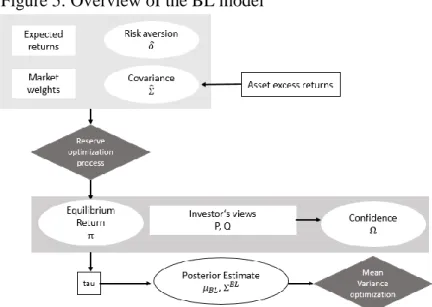
As referred in the previous point, the BL optimization model overcomes major shortcomings of the mean-variance optimization and results in a combining portfolio optimization model with forward-looking investor’s views on the market (Benzschawel and Su, 2015). Figure 5 illustrates an overview of the BL model and all its relevant inputs.
The model begins with the upper right box, which explains the reverse optimization process. The starting inputs are the market weights, a risk aversion parameter, expected excess returns, which are assumed to be the historical average risk-adjusted returns, and finally, an estimated covariance-variance matrix.
The equilibrium returns are determined using reverse optimization, which will be explained in a later section. In a next step, investor can input their views on the market in the BL model (middle portion of Figure 5). Investors usually do not have expertise in every single asset in the portfolio and thus, it is a useful implication of the model that the views do not need to include all assets. The model incorporates investors’ views on asset returns via a projection matrix, a view matrix, and a confidence matrix.14
The expected excess returns can be obtained with the actual BL formula by 𝜇𝐵𝐿= [(τΣ)−1+ 𝑃𝑇Ω−1𝑃]−1[(τΣ)−1𝜋 + 𝑃𝑇Ω−1𝑄]. (11)
14A detailed description of the method whereby investors’ views and confidence are expressed is presented in a
later section of this report
In a final stage, the model uses a Mean-Variance Optimization, but with the BL inputs, in order to find the optimal weights.
6.3. Equilibrium Returns
The BL model uses the equilibrium portfolio as a neutral starting point in which the equilibrium returns clear the market. This means that if all investors hold the same belief, the demand for these assets will exactly equal the outstanding supply (Black and Litterman, 1992). Based on this neutral reference point, the investors can express their views about the market. This reference portfolio has been chosen to be the market capitalization weighted portfolio. By using reserve optimization, one can identify the excess returns implied by the equilibrium portfolio. Usually, the optimization process is used to find the optimal weights given the expected excess returns and the covariance matrix of the portfolio. However, in the reverse optimization process, one is given the variance-covariance matrix and the market weights in order to calculate the expected returns.
Black and Litterman (1992) start the reverse optimization from the utility function given by 𝑈 = 𝑤𝑚𝑘𝑡𝑇 π − (𝛿
2) 𝑤𝑚𝑘𝑡 𝑇 𝛴𝑤
𝑚𝑘𝑡,
where 𝑤𝑚𝑘𝑡 is the vector of market equilibrium weights invested in each asset, π is the vector of equilibrium excess returns for each asset, 𝛿 is the risk aversion parameter, and Σ is the covariance matrix15 of the excess returns for the assets. By taking the first derivative of the utility function with respect to the weights, in the absence of any constraints on the weights and setting the derivative to zero, one will find the maximum of the utility function:
𝜕𝑈
𝜕𝑤 = π − 𝛿𝛴𝑤𝑚𝑘𝑡 = 0
33 Solving now for π, results in the following formula to compute expected excess returns:
π = 𝛿Σ𝑤𝑚𝑘𝑡. (12)
Alternatively, the equilibrium excess returns can be obtained with the CAPM, where the implied excess returns relate to the market portfolio via
π = β × 𝜇𝑀,
where 𝜇𝑀 is the excess return on the market portfolio and β is the vector of asset class betas determined relative to the market’s excess returns. Beta is calculated as
𝛽 =𝐶𝑜𝑣(𝑟, 𝑟𝑇, 𝑤𝑚𝑘𝑡) 𝜎𝑚𝑘𝑡2 =
Σ𝑤𝑚𝑘𝑡 𝜎𝑚𝑘𝑡2 ,
where 𝜎𝑚𝑘𝑡2 represents the variance of the returns of the market portfolio. Substituting beta in the equation for the implied excess returns leads to the reverse optimization formula (Su and Benzschawel, 2015):
π = 𝜇𝑚𝑘𝑡
𝜎𝑚𝑘𝑡2 × Σ𝑤𝑚𝑘𝑡 = 𝛿Σ𝑤𝑚𝑘𝑡.
Given the market weights and the calculation of the covariance matrix, one needs to specify the risk aversion parameter. The risk aversion parameter describes the trade-off between expected risks and expected returns. Satchell and Scowcroft (2000) suggest to calculate 𝛿 with
𝛿 =𝜇𝑚𝑘𝑡 𝜎𝑚𝑘𝑡2 ,
where 𝜇𝑚𝑘𝑡 describes the vector of expected excess return of the market portfolio and 𝜎𝑚𝑘𝑡2 is the variance of the excess market returns.
To calculate the risk aversion parameter based on the CAPM16, one first needs to find an appropriate benchmark to represent the market. In a next step, one computes the expected returns with the following formula:
𝐸(𝑟) = 𝑟𝑓+ 𝛽 ∗ (𝑟𝑚𝑘𝑡− 𝑟𝑓).
The portfolio returns equal the expected returns multiplied by the market cap. Finally, one divides the excess return by the standard deviation of the market caps to reach the risk aversion parameter. With the above mentioned formula, one implements the risk parameter to reach the implied returns.
An issue arises when using the unadjusted historical returns to compute the implied excess returns, as they generate highly volatile sector weights. A technique exists for dampening those fluctuations, called the Bayes-Stein estimator (Jorion, 1986). This estimator performs better than the historical average no matter how one will shrink the individual sector’s sample mean towards the group mean 𝜇̅.
The Bayes-Stein estimator is defined as
𝜇𝐵= (1 − 𝛼)𝜇̂ + 𝛼𝜇̅𝟏 (13)
in which 1 is a 𝑁 × 1 vector of 1’s (assuming 𝑁 ≥ 3), and 𝛼 is a shrinkage factor where 0 < 𝛼 < 1 and equals to
𝛼̂ = 𝑁 + 2
(𝑁 + 2) + 𝑇(𝜇̂ − 𝜇̅x1)′Σ̂−1
(𝜇̂ − 𝜇̅ × 1), (14)
where N is the number of assets, T the number of observations and 𝜇̅ is the average excess return of the sample mean-variance portfolio according to optimal mean-variance portfolio weights:
𝜇̅ = 𝜇̂1𝑤̂1+ 𝜇̂2𝑤̂2+ ⋯ + 𝜇̂𝑁𝑤̂𝑁 (15)
Since, in practice it is common to fix the risk parameter between 2 and 5, we came to the conclusion to do our further calculations with a risk aversion parameter of 2.5, which is the average risk aversion parameter17, in order to obtain more stable results.
17Bodie, Kane and Marcus (2013)
35 6.4. The Black Litterman formula
The BL model of expected excess returns can be expressed as stated in equation (11): 𝜇𝐵𝐿 = [(τΣ)−1+ 𝑃𝑇Ω−1𝑃]−1[(τΣ)−1𝜋 + 𝑃𝑇Ω−1𝑄],
where 𝜇𝐵𝐿 is an Nx1 vector of expected excess returns, τ is a scaling parameter, Σ is a NxN variance-covariance matrix, P is a KxN matrix, whose elements in each row represent the weight of each asset in each of the K view portfolios, Ω is the matrix that represents the confidence in each view, and Q is a Kx1 vector of expected returns of the K view portfolios.
In this form of the BL formula for the expected excess returns, one can see that the returns are a weighted combination of the market equilibrium returns and the expected return implied by the investor’s views. The two weighted matrices are
𝑤𝜋 = [(𝜏Σ)−1+ 𝑃𝑇Ω−1𝑃]−1(τΣ)−1 𝑤𝑞= [(𝜏Σ)−1+ 𝑃𝑇Ω−1𝑃]−1𝑃𝑇Ω−1𝑃.
Specifically, the phrases (τΣ)−1 and 𝑃𝑇Ω−1𝑃 represent the investor’s confidence in the estimates of the market equilibrium and the views, respectively. With a low confidence level in the views, the investor will hold a portfolio which is close to the ones implied by the market equilibrium. Conversely, a high confident investor will invest in a portfolio which deviates from the market portfolio.18
By rearranging the BL formula19, it appears even more clearly the function of 𝜋 as a neutral starting point: 𝜇𝐵𝐿 = 𝜋 + Σ𝑃𝑇× (𝑃Σ𝑃𝑇 +Ω τ) −1 × (𝑄 − 𝑃𝜋). (16)
18 Fabozzi, Focardi and Kolm (2006)
19We refer to Appendix A for the reformulation of 𝜇
The BL vector of expected excess returns is the sum of the equilibrium excess returns plus an additional term, representing the views of investors. In the case when the investor does not have any views about the market, the expected returns implied by the BL model are equal to the equilibrium returns, which allows the investor to hold the market portfolio. However, if the active manager has views about the market, the BL approach combines the information from the equilibrium and pushes the optimal portfolio away from the market portfolio in the direction of the investor’s views.
The estimated variance-covariance matrix refers to the expected excess return from historical data, but it does not correspond to the variance of the actual returns computed by the BL model. Thus, in literature it is suggested to include the BL variance-covariance matrix in the optimization process when calculating the optimal expected excess returns (Benzschawel and Su, 2015). The new variance-covariance matrix is defined as
Σ𝐵𝐿 = (1 + 𝜏)Σ − 𝜏2Σ𝑃′(𝑃𝜏Σ𝑃′+ Ω)−1+ 𝑃Σ. (17)
6.5. Investors’ Views: P, Q and 𝛀 Matrix
One advantage of the BL model is that investors can input their own views, which may differ from the implied equilibrium returns. The model allows such views to be expressed in either absolute or relative terms. However, Idzorek (2005) argues that relative views are more close to the way investment managers feel about different assets. The model does not require the specification of views on all assets and investors are rarely fully confident about their views. The higher the confidence on a view is, the more the model pushes the portfolio towards the investors views. Inversely, the less confident an investor is about his/her views, the more the weights are going to shift towards the equilibrium weights.
37 A view is expressed as a statement that the expected return of a portfolio has a normal distribution with mean equal to Q and a standard deviation of 𝜀. The investors’ views can be represented formally as
𝑃𝜇 = 𝑄 + 𝜀, 𝜖~𝑁(0, Ω), (18)
where 𝜀 is an unobservable normally distributed random vector with zero mean and covariance Ω, which represents a diagonal covariance matrix. The investor’s views are matched to specific assets by matrix P, the “pick” matrix, whose elements in each row represent the weight of each asset in each of the views, as mentioned before. Each expressed view results in a 1xN row vector. Thus, K views result in a KxN P matrix:
𝑃 = [
𝑝1,1 … 𝑝1,𝑁
⋮ ⋱ ⋮
𝑝𝐾,1 ⋮ 𝑝𝐾,𝑁].
Constructing the P matrix, the weights of a relative view will sum up to zero, while for an absolute view the sum will be one. The outperforming assets have a positive value in this matrix, while for the underperforming assets’ the value is negative. There are two different ways to compute the weights within the view. He and Litterman (1999) and Idzorek (2005) use a market capitalization weighed scheme, whereas Satchell and Scowcroft (2000) use an equal weighted scheme in their examples. In the equally weighted scheme, the weighting of each individual asset is proportional to one divided by the number of respective assets outperforming or underperforming. Using the market weighted scheme, one considers the market capitalization. In this scheme the weightings are proportional to the asset’s market capitalization divided by the total market capitalization of either the outperforming or underperforming assets of that particular view. Within the P matrix, a zero is displayed when a certain asset is not included in the view.
The Q vector states investors’ expected returns regarding the market performance, which are different from the implied equilibrium returns in a Kx1 vector. The uncertainty of the views