Efficient domination through eigenvalues
Domingos M. Cardoso
∗Vadim V. Lozin
†Carlos J. Luz
‡Maria F. Pacheco
§Abstract
The paper begins with a new characterization of (k, τ)-regular sets. Then, using this result as well as the theory of star complements, we derive a simplex-like algorithm for determining whether or not a graph contains a (0, τ)-regular set. Whenτ = 1, this algorithm can be applied to solve theefficient dominating setproblem which is known to be
NP-complete. If−1 is not an eigenvalue of the adjacency matrix of the graph,
this particular algorithm runs in polynomial time. However, although it doesn’t work in polynomial time in general, we report on its successful application to a vast set of randomly generated graphs.
AMS classification 05C50
Keywordsefficient dominating set, dominating induced matching, (k, τ)-regular sets, graph eigenvalue.
1
Introduction
All graphs in this paper are undirected, without loops and multiple edges. The vertex set of a graph G is denoted V(G) and its edge set E(G). The com-plementary graph ¯Gof G is the graph with the same vertex set as G, where any two distinct vertices are adjacent if and only if they are not adjacent inG.
The open neighbourhood NG(v) of a vertex v ∈ V(G) is the set of its
neigh-bours, i.e., the set of vertices adjacent tov,and theclosed neighbourhood ofvis
N[v] ={v} ∪N(v). Thedegree dG(v) ofvis the number of its neighbours inG,
∗Center for Research and Development in Mathematics and Applications, Department of
Mathematics, University of Aveiro, E-mail: [email protected].
†Mathematics Institute, University of Warwick, UK. E-mail: [email protected]. This
author gratefully acknowledges support from DIMAP – the Center for Discrete Mathematics and its Applications at the University of Warwick, and from EPSRC, grant EP/L020408/1.
‡Center for Research and Development in Mathematics and Applications, University of
Aveiro, E-mail: [email protected].
§Center for Research and Development in Mathematics and Applications, University of
i.e.,dG(v) =|NG(v)|(in general, given a finite setS,the number of elements of
Swill be denoted by|S|). GivenX ⊆V(G),the subgraph ofGinducedbyX is the graph whose vertices are the elements ofX and whose edges are the edges ofGthat link vertices ofX. If all vertices of Ghave the same degreer,we say thatGisr-regular or simplyregular. A subsetS⊆V(G) is anindependent set
if no pair of vertices inS is connected by an edge.
Given a vertexv in a graphG, we say thatvdominates all vertices inN[v]. A setS of vertices ofGisdominating if every vertex ofGoutsideS is adjacent to at least one vertex of S. The domination number of a graph G, denoted
γ(G), is the minimum size of a dominating set of vertices inG. A dominating set S is anefficient dominating set (or independent perfect dominating set) if each vertex of Gis dominated by precisely one vertex of S or, equivalently, if the minimum length of a path between any two vertices ofSis at least three. It is not difficult to see that not every graph has an efficient dominating set (take, for example, C4, i.e., a cycle on four vertices). In [1], Bange, Barkauskas and
Slater (see also [25]) showed thatS={s1, s2, . . . , sk}is an efficient dominating
set of G if and only if {N[s1], N[s2], . . . , N[sk]} is a partition of V(G). They
also showed that, ifG has an efficient dominating set then the cardinality of any efficient dominating set equals the domination number γ(G) of G. As a consequence, all efficient dominating sets ofGhave the same cardinality.
The efficient dominating set problem (or simply efficient domina-tion) is the problem of determining whether a given graph has an efficient
dom-inating set and finding such a set if it exists. There are many applications for efficient domination in coding theory [2, 24], graph embedding [35, 36], facility location on geographical areas [37] and resource allocation in parallel processing systems [27, 28, 32]. It was proved in [1] that the efficient domination problem is NP-complete for general graphs. The same conclusion has been reached for many very restricted graph families such as bipartite graphs [37], chordal graphs [37], chordal bipartite graphs [31], planar graphs of maximum degree three [22], planar bipartite graphs [31] and many other special families, see e.g. [7, 31]. On the other hand, for graphs in several special classes, efficient domination
can be solved in polynomial-time (for a list of these special classes of graphs see e.g. [3, 4, 5, 7, 18, 26, 31, 32]).
A problem which is closely related to efficient domination is that of
determining ifGhas anefficient edge dominating set, i.e., a setSof edges such that every edge ofGshares a vertex with precisely one edge inS(assuming that an edge shares a vertex with itself). This problem is also NP-complete in general [23] and received considerable attention in the literature under several names, such asefficient edge dominationordominating induced matching(see
e.g. [6, 8, 9, 13, 14, 16, 29, 30]). An instance of efficient edge domination
can be transformed into an instance of efficient dominationby associating
to the input graphGits line graphL(G), in which case the edges ofGbecome the vertices ofL(G) with two vertices being adjacent inL(G) if and only if the respective edges ofGshare a vertex. As a consequence,efficient domination
✟✟❍❍✟✟ ❍
❍ ✂
✂ ✂
❇ ❇
❇ ❇ ❇ ❇❇
✔✔ ✂✂
✂✂
❚ ❚ ✑ ✑ ✑
◗
◗◗
s s s s
s s
s s
s s
3 4 9 10
6
7 8
5
1 2
Figure 1: The vertex subsetsS1 ={1,2,3,4}, S2 ={5,6,7,8,9,10} and S3 =
{1,2,5,7,8} are (0,2)-regular, (1,3)-regular and (2,1)-regular, respectively.
An efficient dominating set can also be defined as follows: a setS of vertices of a graph G is an efficient dominating set if S induces in Ga regular graph of degree 0 (i.e.,S is an independent set) and every vertex ofGoutsideS has precisely one neighbour inS. In the terminology of [11] (see also [12] and [15]), a setS satisfying this property is called a (0,1)-regular set.
More generally, a subsetS ⊆V(G) is a (k, τ)-regular set inG if it induces ak-regular subgraph inGand every vertex outsideS has exactlyτ neighbours in S. We will assume that k is a nonnegative integer and that τ is always a positive integer with the following exception: when a graphGisr-regular,V(G) is considered by convention a (r,0)-regular set. For example, in the Petersen graph depicted in Figure 1, the set S1 = {1,2,3,4} is (0,2)-regular, the set
S2 = {5,6,7,8,9,10} is (1,3)-regular and the set S3 = {1,2,5,7,8} is (2,
1)-regular. As well, the vertex set of the Petersen graph is a (3,0)-regular set by convention. Some results on the existence of (k, τ)-regular sets have been obtained by means of spectral graph theory in [11, 12, 15].
Since an efficient dominating set can be viewed as a (0,1)-regular set, effi-cient dominationis a particular case of the general problem of determining
whether a graph contains a (0, τ)-regular set. In this paper, using some spec-tral results on (k, τ)-regular sets as well as the theory of star complements, we present a simplex-like algorithm for detecting a (0, τ)-regular set in an arbitrary graph. This general approach will subsequently be applied toefficient dom-ination. Although this particular algorithm can be used to find an efficient
dominating set in any given graph or to conclude that such a set doesn’t ex-ist, it is not polynomial in general. However, if−1 is not an eigenvalue of the adjacency matrix of the graph, it works in polynomial time.
The remaining sections of this paper are organized as follows. In Section 2, additional notation is given and some preparatory results on (k, τ)-regular sets needed in the sequel are presented. Namely, a new characterization of (k, τ)-regular sets is proposed. Next, in Section 3, we recall some facts from the theory of star complements and use them to describe a simplex-like algorithm for detecting (0, τ)-regular sets. In Section 4, considering τ = 1, the referred simplex-like algorithm is applied to efficient dominating. Finally, in
containing at least two efficient dominating sets and also a series of bipartite graphs.
2
Preparatory results
We first introduce some more notation that will be needed below.
The adjacency matrix A(G) = [aij] of a graph G of order n is the n×n
matrix defined byaij= 1 if (vi, vj)∈E(G) andaij= 0 otherwise. This matrix
is real and symmetric and all itsneigenvaluesλ1≥. . .≥λn are real numbers.
The eigenvalues ofA(G) are also called the eigenvalues of G. The spectrum of
A(G) (also called the spectrum of G) is represented by σ(G). The eigenspace of an eigenvalueλ∈σ(G) is denoted byEG(λ) = ker(A(G)−λIn) (in general,
given a natural numbern,In represents the identity matrix of ordern; we also
use ker(M) to denote the kernel or null space of a matrixM). The dimension of
EG(λi) coincides with the multiplicity of λi, which will be denoted bymG(λi).
Recall also that ifGhas at least one edge, thenA(G) has a negative eigenvalue not greater than−1 and a positive eigenvalue not less than the average degree inG[20].
Throughout the paper, all considered vectors are column vectors. They will be represented in boldface as for example x = (x1, . . . , xn)
T
, that denotes a vector ofRn(T stands for the transposition operation),jthat will represent the
all-one vector or0that denotes the null vector.
We turn now to the presentation of the results on (k, τ)-regular sets needed in the sequel. The following criterion for the existence of a (k, τ)-regular set is a slight variation of Proposition 2.2. of [11]. The proof is given for the sake of completeness.
Proposition 2.1 A graphGof ordernhas a(k, τ)-regular setS if and only if the system
(A(G)−(k−τ)In)x=τj, (1) has a 0-1 solution. Furthermore, such a solutionx= (x1, . . . , xn)T is the cha-racteristic vector ofS (i.e., xi= 1if i∈S andxi= 0 otherwise).
Proof. Let us assume that G has a (k, τ)-regular set. Then by Proposition 2.2 of [11], its characteristic vector is a solution of (1) and hence there is a 0-1 solution. Conversely, assume that the system (1) has a 0-1 solutionxand define the vertex subsetS={vi:xi= 1}. Since, from (1),
X
j∈NG(i)∩S
xj−(k−τ)xi=τ⇔ |NG(i)∩S|= (k−τ)xi+τ, fori= 1, . . . , n,
we may conclude that
|NG(i)∩S|=
k ifvi ∈S
and thereforeS is a (k, τ)-regular set.
The characteristic vectors of (k, τ)-regular sets were studied in Proposition 4.1 and Corollary 4.3 of [15]. Based on different tools, namely the minimal least squares solution of a linear system, we next give a result that subsumes and is equivalent to the above cited statements of [15]. To facilitate the reading, we present the proof of this equivalence in the appendix.
Proposition 2.2 Let G be a graph of order n with at least one (k, τ)-regular set and denote byx+ the minimal least squares solution of system (1).
Then a subset S ⊆V(G) is a (k, τ)-regular set in G if and only if its cha-racteristic vectorx is such that
x=x++q, (2)
whereq=0if(k−τ)∈/ σ(G)andq∈ EG(k−τ)otherwise. Moreover,
x+=
(A(G)−(k−τ)In)−1(τj) if (k−τ)∈/σ(G) n−t
X
i=1
τ j
Tu i
λi−(k−τ)
ui if (k−τ)∈σ(G) , (3)
wheret= dimEG(k−τ), λ1, . . . , λn−tare the eigenvalues ofA(G)different from
k−τ andu1, . . . ,un−t are corresponding mutually orthonormal eigenvectors.
Proof. First, notice that x+ is a solution of the system (1) and from
Proposi-tion 2.1S⊆V(G) is (k, τ)-regular if and only if its characteristic vectorxis also a solution of the system (1), that is, if and only if∃q∈ker(A(G)−(k−τ)In)
such thatx =x++q. Saying that q belongs to the null space of the matrix
A(G)−(k−τ)In is equivalent to saying thatq is an eigenvector of A(G)
as-sociated to the eigenvalue (k−τ) when (k−τ)∈σ(G) andq=0 otherwise. Therefore, the first part of the proposition is proven.
It remains to prove that x+ = nP−t
i=1
τ jTui
λi−(k−τ)ui when (k−τ) ∈ σ(G). Let
Un−t be the matrix whose columns are the eigenvectors u1, . . . ,un−t and let
Dn−t be the diagonal matrix whose diagonal entries are λi −(k−τ), i =
1, . . . , n−t.Since
A(G)−(k−τ)I=Un−tDn−tUnT−t,
considering the Moore-Penrose generalized inverse ofA(G)−(k−τ)I (see for instance [10]) which is usually denoted by (A(G)−(k−τ)I)† it follows that
(A(G)−(k−τ)I)†= Un−tDn−tUnT−t
†
=Un−tDn−−1tU T n−t=
n−t
X
i=1
1
λi−(k−τ)
uiuTi.
Therefore,x+= (A(G)−(k−τ)I)†
(τj) =
n−t
P
i=1
τ jTui
We complete this section by noting that if G has a (k, τ)-regular set, its size can easily be computed as it is stated in the following corollary of Proposi-tion 2.2.
Corollary 2.2.1 If a graph G has a (k, τ)-regular set S ⊆V(G), then |S| =
jTx+.
Proof. If S ⊆V(G) is (k, τ)-regular set in G, then its characteristic vectorx
satisfies x =x++q. If q = 0, |S| = jTx =jTx+ and the corollary follows.
Otherwise, (A(G)−(k−τ)In)x=τjimplies thatjTq=0,i.e.,qis orthogonal
to the all-one vectorj.Therefore,|S|=jTx=jTx++jTq=jT
x+.
This corollary provides an easy sufficient condition for the non-existence of a (k, τ)-regular set.
Corollary 2.2.2 IfjTx+ is not a natural number, thenGhas no(k, τ)-regular
set.
3
Detecting
(0
, τ
)
-regular sets
According to Proposition 2.1, detecting a (0, τ)-regular set in a graphGof order
nis equivalent to search for a 0-1 solution of (A(G) +τ In)x=τj.Note that, if
any solutionx of this system is nonnegative, thenx ≤j. In fact, this system can be written in the form
τ xi+
X
k∈NG(i)
xk=τ, i= 1, . . . , n;
thus, ifx≥0,we have, for alli, τ xi≤τ,and thenxi≤1 sinceτ >0. Therefore,
the set of solutions of the system
(A(G) +τ In)x = τj
x ≥ 0 (4)
is included in the hypercube [0,1]n. Then, obtaining a (0, τ)-regular set inGis
equivalent to determining an extreme vertex of the convex polyhedron [0,1]n.
The theory of star complements allows us to link the 0-1 solutions of (4) and, more generally, its basic feasible solutions with the star set concept (see below). We begin this section by recalling some basic facts of that theory.
3.1
Star sets and star complements
Given a graph G, let λ be an eigenvalue of G with multiplicity k > 0 and
EG(λ) its eigenspace. Also, if X is a subset of V(G), ¯X = V(G)\X is its
complementary set andG−X is the subgraph ofGinduced by ¯X. We say that
X is a star set for λin G (or simply aλ-star set) if |X|=k and λis not an eigenvalue ofG−X.In addition, ¯X =V(G)\X is called aλ-co-star set, while
The next proposition follows directly from the proof of Theorem 5.1.7 in [21] which is known as the Reconstruction Theorem.
Proposition 3.1 Given a graph G of orden n, let X ⊂ V(G), X¯ =V(G)\X
and A(G) =
AX NT
N CX¯
, where AX and CX¯ are the adjacency matrices of
the subgraphs induced byX andX¯, respectively. ThenX is aλ-star set ofGiff
λis not an eigenvalue of CX¯ and the rows of
h
N CX¯ −λI|X¯|
i
form a basis of the row space ofA(G)−λIn. Furthermore,EG(λ)is spanned by the vectors
" y
−CX¯−λI|X¯|
−1
Ny #
, (5)
wherey∈R|X|.
It should be noted that, from the definition of a star set, we may conclude that for every graphGand every eigenvalueλofGthere is at least oneλ-star set.
We recall another basic result from the theory of star complements also given in [21].
Proposition 3.2 LetGbe a graph,λone of its eigenvalues,X aλ-star set and
¯
X =V(G)\X the corresponding co-star set. If λ6= 0, thenX¯ is a dominating set forG.
3.2
A simplex-like approach
In this subsection we describe a simplex-like algorithm for the detection of (0, τ )-regular sets in a graphGwhen λ=−τ ∈σ(G). Note that if λ=−τ /∈σ(G), obtaining the unique solution of (A(G) +τ In)x=τjis sufficient to decide ifG
has or not a (0, τ)-regular set.
From Proposition 3.1, assumingX is a star set forλ=−τ ∈σ(G) inG,we conclude that system (4)is equivalent to the system:
N CX¯ +τ I|X¯|
x = τjX¯
x ≥ 0 , (6)
where jX¯ denotes the subvector of j whose entries are indexed by ¯X. Notice
that (6) is a subsystem of (4) just formed by the equation associated to the indices in ¯X. Let us call x a star solution of (6) if x solves this system and there exists a star setX forλ=−τ in Gsuch that xi = 0 ifi ∈X. We now
state a result that slightly generalizes Theorem 14 of [17].
Theorem 3.3 Let Gbe a graph, λ=−τ ∈σ(G)andX a star set for λ=−τ
Proof. Theorem 14 of [17] proves the same assertion for system (6) when
λ= −τ is the least eigenvalue of G. It happens that the same proof holds if instead we consider any other eigenvalueλ=−τ ∈σ(G).
In other words, the last theorem asserts that every vertex subset ¯X′⊂V(G)
is a co-star set for the eigenvalue λ = −τ if and only if the columns of the matrix
N CX¯ +τ I|X¯|
whose indices are in ¯X′ define a basic submatrix of
(6). The next result guarantees that the search for a 0-1 solution of (6) can be limited to its star solutions, i.e., to its basic feasible solutions (this amounts to say that it suffices to search on some of the co-star sets forλ=−τ).
Proposition 3.4 Every 0-1 solution of the system (6) is a basic feasible solu-tion.
Proof. The polytope defined by (6) is included in the hypercube [0,1]n.
There-fore, each 0-1 solution is an extreme vertex of this hypercube and thus a basic feasible solution.
Based on the above results, we may apply a simplex technique to system (6) for deciding whether this system has or not a 0-1 solution (i.e., for deciding is
Ghas or not a (0, τ)-regular set). We may start from the simplex tableau
xN
xB (CX¯′+τ IX¯′)
−1
N τ(CX¯′+τ IX¯′)
−1
jX¯′ (7)
whereX′is some star set for−τinG(which defines the indices of the nonbasic
variablesxN) and ¯X′=V(G)\X defines the indices of the basic variablesxB.
It should be noted that the initial star solution (xB, xN) and the correspondent
star set X′ can be obtained by first computing a feasible solution of (6) and subsequently applying the nullifying procedure described in [17] and analized in Theorem 12 of that paper. Thus, if the right-hand side of (7) is nonnegative but not integer, we may apply the fractional dual algorithm for Integer Linear Programming (ILP) with Gomory cuts (described for example in [33]) until a 0-1 star solution is determined or the conclusion that such solution does not exist is obtained.
4
An algorithm for efficient domination
As mentioned in the Introduction, an efficient dominating set can be viewed as a (0,1)-regular set. Consideringτ= 1, we now apply toefficient domination
the simplex-like approach for detecting (0, τ)-regular sets given in Section 3. Before proceeding we introduce an upper bound for the size of an efficient dom-inating set using the star complement theory.
Proposition 4.1 LetGbe a graph of ordern. IfGhas an efficient dominating setS, then
Proof. Recalling what has been said in the Introduction, |S| = γ(G). By Proposition 3.2, any co-star set ¯X for any eigenvalue λ6= 0 is a dominating set forG.As
X¯
=n−mG(λ),the result follows.
Now, specializing the results of Section 2 to efficient dominating sets we obtain:
Proposition 4.2 Let G be a graph of order n, consider k= 0 andτ = 1 and
x+ given by (3). Then:
1. If Ghas an efficient dominating set S⊆V(G), then|S|=jTx+.
2. If jTx+ is not a natural number, then Ghas no efficient dominating set.
3. If −1 ∈/ σ(G), G has an efficient dominating set if and only if the com-ponents of x+ are 0-1. Furthermore, if x+ is a 0-1 vector then it is the
characteristic vector of the unique efficient dominating set of G.
Proof. Proposition 2.2 and its corollaries imply facts 1, 2 and the first part of 3. To prove the last part of fact 3, assume that there are two distinct (0, 1)-regular sets S and S′ with characteristic vectors x and x′, respectively; then q=x−x′∈ker(A(G) +I
n)\{0},i.e.,−1∈σ(G) which is a contradiction.
Based on this proposition and taking into account Subsection 3.2, we give below Algorithm 1 for theefficient domination problem. Notice that the
step 3 of Algorithm 1 guarantees that it stops if −1 ∈/ σ(G). Clearly in this case the algorithm works in polynomial time. Otherwise, although we have no guarantee of polynomiality, the Algorithm 1 is finite since the fractional dual algorithm for ILP with Gomory cuts (steps 5–7) is finite too. Since, by Proposition 3.4, all 0-1 solutions are basic, we can assert the correctness of the output produced by the algorithm in step 8.
s s
s
s s
s s
s 1
3
2
4 5
7
6 8
✑✑✑ ❅
❅❅ ✑ ✑ ✑
❅ ❅ ❅
◗ ◗ ◗
◗ ◗◗
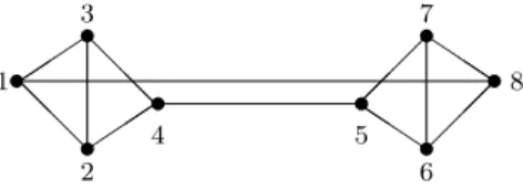
Figure 2: GraphGwithσ(G) ={3,√5,1,−1,−√5}, wheremG(−1) = 4
.
Example 4.1 Let us apply the Algorithm 1 to the graphGdepicted in the figure 2 to decide ifGhas or not a (0,1)-regular set.
1: Since the graph G is 3-regular, it is immediate that x+ = 1
4j8, where j8
denotes an all-one vector with eight entries.
Algorithm 1(forefficient domination).
Require: The adjacency matrix of a graphGof ordern.
Ensure: The characteristic vector of an efficient dominating set of G or the conclusion that such vertex subset does not exists.
1: Determine thex+ vector given in (3).
2: if jTx+6∈Nthen STOP(Ghas no efficient dominating set)end if.
3: if−1∈/ σ(G)thenreturn the output obtained from fact 3 of Proposition 4.2 andSTOP end if.
4: Determine a co-star set for the eigenvalue −1 and the associated simplex tableau (7).
5: while no conclusion about the existence of a 0-1 solution is obtained from
the simplex tableaudo
6: Apply the fractional dual algorithm for ILP with Gomory cuts. 7: end while
8: if the fractional dual algorithm stopped with a 0-1 solution then return such solution as the characteristic vector of an efficient dominating setelse
return the conclusion thatGhas no efficient dominating setend if.
3: Since mG(−1) = 4we proceed for the next step;
4: Since the vertex subset X¯ ={4,5,7,8} is a co-star set for the eigenvalue
−1, then the matrix
N CX¯ +τ I|X¯|
associated to this co-star set takes the form
1 2 3 6 4 5 7 8
4 0 1 1 0 1 1 0 0
5 0 0 0 1 1 1 1 0
7 0 0 0 1 0 1 1 1
8 1 0 0 1 0 0 1 1
,
and the corresponding simplex tableau (7) is
x1 x2 x3 x6
x4 1 1 1 0 1
x5 −1 0 0 0 0
x7 0 −1 −1 1 0
x8 1 1 1 0 1
6: The obtained solution is feasible and 0-1;
8: Therefore,S={4,8} is an efficient dominating set forG.
5
Computational experiments
We have tested Algorithm 1 on two groups of randomly generated graphs, namely a series of bipartite graphs and a set of graphs with eigenvalue −1 containing at least two efficient dominating sets (recall that this case is the in-teresting one since, for graphs without eigenvalue−1,the efficient domination problem is easily solved by Algorithm 1).
The last set of graphs was generated taking into account Theorem 2.5 of [20]:
If the spectrum of the graphGcontains an eigenvalueλ0with multiplicityp >4,
then the spectrum of the complementary graphG¯contains an eigenvalue −λ0−1
with multiplicityq,wherep−1≤q≤p+1.Thus, departing from a null graphG0
with a predefined number of vertices as well as from a predefined cardinality, two different efficient dominating sets with this cardinality were randomly generated and implanted inG0 giving rise to graph G1; then, for a predefined density, a
random graphG2 was generated (see for instance [19, p. 376]) on the vertices
ofG1 that don’t belong to any of the two implanted efficient dominating sets.
Next, 5 vertices were duplicated in ¯G2allowing us to obtain a graph, denoted by
G3,which necessarily has the eigenvalueλ0= 0 with multiplicity at least 5; the
above cited Theorem 2.5 of [20] finally guarantes that the complementary graph ¯
G3 has−1 as a eigenvalue with multiplicity at least 4. Algorithm 1 was applied
to the graphs ¯G3generated as described. Table 1 summarizes some of obtained
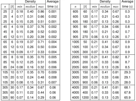
results. Its first column, denoted by “n”, lists the twelve different graph orders considered, ranging fromn= 25 until n= 4005 vertices. The second column, denoted by “|S|”, presents three different cardinalities of the generated efficient dominating setsSfor each considered value ofn.The next three columns report on the densities of the generated graphs; it should be noted that, for eachnand
|S|,thirty instances were generated according to three predefined density levels (namely the 0.25, 0.5 and 0.75 densities); the density columns of the table show the minimum, median and maximum of the set of final densities reached by each of the thirty instances. Finally, the last column gives the average time (in seconds) spent by the algorithm on each set of thirty instances.
Note that Table 1 reports on results of applying Algorithm 1 for altogether 1080 randomly generated graphs. The tests were carried out on a computer using an Intel(R) Core(TM) i7-3770K/3.50GHz processor with 16.0 Gb RAM and Windows 7 (64 bits) as the operating system. The overall procedure was implemented in MATLAB (version 7.6), where the built-in functionsrandperm
andrandwere respectively called to randomly generate the implanted efficient dominating sets and the graph induced by the remaining vertices.
the determination of a co-star set associated to the eigenvalue−1 immediately yielded a 0-1 solution and consequently an efficient dominating set. Although this perhaps explains the low running times observed, it can also be a motiva-tion for future work to try understand the reasons of this behaviour. However, as a conclusion, we can say that Algorithm 1 is very suitable for solving the effi-cient domination problem in large graphs generated according to the foregoing procedure.
Density Average
n |S| min median max time (s)
25 2 0.18 0.40 0.86 0.001 25 4 0.17 0.31 0.66 0.002
25 6 0.15 0.25 0.51 0.001 45 4 0.19 0.37 0.76 0.002 45 8 0.15 0.28 0.52 0.003
45 12 0.11 0.20 0.39 0.002 65 6 0.19 0.37 0.71 0.004 65 12 0.13 0.26 0.50 0.004
65 18 0.09 0.17 0.33 0.004 85 8 0.18 0.35 0.70 0.005 85 16 0.12 0.25 0.51 0.006 85 24 0.08 0.16 0.32 0.006
105 10 0.17 0.35 0.70 0.009 105 20 0.12 0.24 0.48 0.008 105 30 0.08 0.15 0.31 0.007
305 30 0.17 0.34 0.67 0.06 305 60 0.11 0.22 0.44 0.06 305 90 0.07 0.14 0.29 0.06
Density Average
n |S| min median max time (s)
605 60 0.17 0.34 0.67 0.3
605 120 0.11 0.21 0.43 0.3
605 180 0.07 0.13 0.26 0.3
905 90 0.17 0.34 0.66 0.8
905 180 0.11 0.21 0.42 0.7
905 270 0.06 0.13 0.26 0.7
1005 50 0.21 0.41 0.82 0.9
1005 100 0.17 0.34 0.67 0.9
1005 300 0.07 0.13 0.27 0.9 2005 100 0.21 0.41 0.82 8.7 2005 200 0.17 0.33 0.66 8.7 2005 600 0.06 0.13 0.26 8.5
3005 150 0.21 0.41 0.81 29.3 3005 300 0.17 0.33 0.66 29.1 3005 900 0.06 0.13 0.25 28.0
4005 200 0.21 0.41 0.81 68.1 4005 400 0.17 0.33 0.66 67.8 4005 1200 0.06 0.13 0.25 65.9
Table 1: Some computational results for randomly generated graphs with at least two efficient domination sets
the number of those with eigenvalue−1,respectively. Finally, the average time (in seconds) spent by the algorithm for each group of 600 bipartite graphs is reported.
Some similarities were observed between the tests with bipartite graphs and those first described in this section. In fact, in the present case, the graph density also seems to be uncorrelated with the time spent by the algorithm, which continues to be heavily dependent of graph order. In addition, the determination of a co-star set associated to the eigenvalue−1 immediately yielded an efficient dominating set, preventing the use of Gomory cuts. Finally, the low running times observed grants to the Algorithm 1 a promising practical value.
Density Without With With With Average
n min median max eds V=?1 eds V=?1 time (s)
20 0.03 0.27 0.53 418 8 182 39 0.004 50 0.02 0.25 0.51 390 2 210 144 0.006 100 0.01 0.25 0.51 399 4 201 182 0.013 300 0.01 0.24 0.50 408 4 192 178 0.124 500 0.01 0.24 0.50 424 6 176 148 0.393 1000 0.01 0.25 0.50 586 23 14 4 4.352
Table 2: Some computational results for randomly generated bipartite graphs
References
[1] D.W. Bange, A.E. Barkauskas, P.J. Stater, Efficient dominating sets in graphs, inRingeisen, R.D. and Roberts, F.S. (eds.) Applications of Discrete Mathematics, SIAM, Philadelphia, PA (1988), 189–199.
[2] N. Biggs, Perfect codes in graphs,J. Combinatorial Theory (B),15(1973), 289–296.
[3] A. Brandst¨adt, Weighted Efficient Domination forP5-Free Graphs in Linear
Time, arXiv:1507.06765v1, (2015).
[4] A. Brandst¨adt, E.M. Eschen, E. Friese, Efficient Domination for Some Sub-classes ofP6-Free Graphs in Polynomial Time, extended abstract accepted
for WG 2015. Full version: arXiv:1503.00091v1, (2015).
[5] A. Brandst¨adt, V. Giakoumakis, Weighted Efficient Domination for (P5+
[6] A. Brandst¨adt, C. Hundt, R. Nevries, Efficient edge domination on hole-free graphs in polynomial time. LATIN 2010: Theoretical Informatics, Lecture Notes in Comput. Sci., Springer, Berlin,6034 (2010), 650–661.
[7] A. Brandst¨adt, M. Milani´c, R. Nevries, New polynomial cases of the weighted efficient domination problem, extended abstract in: Conference Proceedings of MFCS 2013. Full version: arXiv:1304.6255v1,LNCS 8087
(2013), 195–206.
[8] A. Brandst¨adt, R. Mosca, Dominating Induced Matchings for P7-Free
Graphs in Linear Time,Algorithmica,68(4) (2014), 998–1018.
[9] A. Brandst¨adt, B. Leitert, D. Rautenbach, Efficient Dominating and Edge Dominating Sets for Graphs and Hypergraphs, arXiv:1207.0953v2.
[10] S. L. Campbell, C. D. Meyer Jr., Generalized Inverses of Linear Transfor-mations, corrected reprint of the 1979 original, Dover Publications, New York (1991).
[11] D. M. Cardoso, P. Rama, Equitable bipartitions of graphs and related results,Journal of Mathematical Sciences,120(2004), 869–880.
[12] D. M. Cardoso, P. Rama, Spectral results on regular graphs with (k, τ )-regular sets,Discrete Math.,307(2007), 1306–1316.
[13] D. M. Cardoso, J. O. Cerdeira, C. Delorme, P. C. Silva, Efficient edge domination in regular graphs, Discrete Applied Mathematics, 156 (2008), 3060-3065.
[14] D. M. Cardoso, V. V. Lozin, Dominating induced matchings, in Lip-shteyn, Marina (ed.) et al., Graph theory, Computational Intelligence and Thought. Essays dedicated to Martin Charles Golumbic on the occasion of his 60th birthday. Springer, Berlin, Lecture Notes in Computer Science,
5420 (2009), 77–86.
[15] D. M. Cardoso, I. Sciriha, C. Zerafa, Main eigenvalues and (k, τ)-regular sets, Linear Algebra Appl.,423(2010), 2399–2408.
[16] D. M. Cardoso, N. Korpelainen, V. V. Lozin, On the complexity of the dom-inating induced matching problem in hereditary classes of graphs,Discrete Appl. Math.,159(2011), 521–531.
[17] D. M. Cardoso, C. J. Luz, A simplex like approach based on star set for recognizing convex-QP adverse graphs, J. Comb. Optim., in press, DOI 10.107/s10870-014-9745-x.
[19] G. Chartrand, L. Lesniak, Graphs & digraphs, 4th Edition, Chapman & Hall/CRC, Boca Raton, FL, (2005), viii+386 pp.
[20] D. Cvetkovi´c, M. Doob, H. Sachs,Spectra of Graphs,Academic Press, New York (1979).
[21] D. M. Cvetkovi´c, P. Rowlinson, S. Simi´c,An Introduction to the Theory of Graph Spectra, Cambridge University Press, Cambridge (2010).
[22] M. R. Fellows, M.N. Hoover, Perfect Domination, Austral. J. Combin., 3
(1991), 141–150.
[23] D. L. Grinstead, P. L. Slater, N. A. Sherwani, N. D. Holmes, Efficient edge domination problems in graphs,Information Processing Letters,48(1993), 221–228.
[24] P. Hammond, D. Smith, Perfect codes in the graphsQk,J. Combin. Theory Ser. B, 19(1975), 239–255.
[25] T.W. Haynes, S.T. Hedetniemi, P.J. Slater, Fundamentals of Domination in Graphs, Marcel Dekker, New York, (1998).
[26] Y.D. Liang, C.L. Lu, C.Y. Tang, Efficient domination on permutation graphs and trapezoid graphs, Lecture Notes in Computer Science, 1276
(1997), 232–241.
[27] M. Livingston, Q.F. Stout, Distributing resources in hypercube computers,
Proceedings of the Third Conference on Hypercube Concurrent Computers and Applications, (1988), pp. 222–231.
[28] M. Livingston, Q.F. Stout, Perfect dominating sets, Congr. Numer., 79
(1990), 187–203.
[29] C.L. Lu, M.-T. Ko, C.Y. Tang, Perfect edge domination and efficient edge domination in graphs,Discrete Applied Math.,119(2002), 227–250.
[30] C.L. Lu, C.Y. Tang, Solving the weighted efficient edge domination problem on bipartite permutation graphs, Discrete Applied Math.,87(1998), 203– 211.
[31] C.L. Lu, C.Y. Tang, Weighted efficient domination problem on some perfect graphs, Discrete Applied Math.117(2002), 163–182.
[32] M. Milaniˇc, Hereditary Efficiently Dominatable Graphs, available online in:
Journal of Graph Theory, (2012).
[33] C. H. Papadimitriou, K. Steiglitz, Combinatorial Optimization: Algorithms and Complexity, Dover Publications, (1998).
[35] P.M. Weichsel, Distance regular subgraphs of a cube,Discrete Math.,109
(1992), 297–306.
[36] P.M. Weichsel, Dominating sets inn-cubes, J. Graph Theory 18, (1994), 479–488.