Consumer confidence, endogenous growth and endogenous cycles

Consumer Confidence, Endogenous Growth and

Endogenous Cycles

Orlando Gomes

∗

Escola Superior de Comunicação Social [Instituto Politécnico de Lisboa] and Unidade de Investigação em Desenvolvimento Empresarial [UNIDE/ISCTE].

- January, 2007 -

Abstract: Endogenous growth models are generally designed to address long term trends of

growth. They explain how the economy converges to or diverges from a balanced growth path and they characterize aggregate behaviour given the optimization problem faced by a representative agent that maximizes consumption utility. In such frameworks, only potential output matters and all decisions, by firms and households, are taken assuming that any output gap does not interfere with the agents’ behaviour. In this paper, we develop growth models (without and with optimization) that depart from the conventional framework in the sense that consumption decisions take into account output fluctuations. Households will raise their propensity to consume in periods of expansion and they will lower it in phases of recession. Such a framework allows to introduce nonlinear features into the model, making it feasible to obtain, for reasonable parameter values, endogenous fluctuations. These are triggered by a Neimark-Sacker bifurcation.

Keywords: Endogenous growth, Endogenous business cycles, Nonlinear dynamics,

Neimark-Sacker bifurcation.

JEL classification: O41, E32, C61.

∗ _{Orlando Gomes; address: Escola Superior de Comunicação Social, Campus de Benfica do IPL,}

1549-014 Lisbon, Portugal. Phone number: + 351 93 342 09 15; fax: + 351 217 162 540. E-mail: ogomes@escs.ipl.pt.

Acknowledgements: Financial support from the Fundação Ciência e Tecnologia, Lisbon, is grateful acknowledged, under the contract No POCTI/ECO/48628/2002, partially funded by the European Regional Development Fund (ERDF).

1. Introduction

Standard growth models commonly overlook any possible reaction of households relatively to short run economic performance (i.e., to business cycles). Such growth models are long term paradigms, where a permanent coincidence between effective output and potential output is implicitly assumed. In this paper, we reinterpret the conventional AK endogenous growth model when this is modified to include consumers’ response to previous periods’ deviations of output relatively to its potential level. This response relates to a simple mechanism that involves confidence: when the output gap in the previous periods is systematically positive, demand side agents become increasingly confident, and they will consume an amount of resources that is tendencially higher than the consumption level derived from the benchmark growth models (the optimal consumption level of a Ramsey-like setup or the consumption level that arises from assuming a constant marginal propensity to save); if, alternatively, the observed output gap in the near past corresponds to negative value, then the contemporaneous level of consumption falls below the reference level.

The described mechanism intends to add realism to the simple growth model. It is well accepted by the economics profession that households in fact take into account short term macroeconomic fluctuations in order to plan their income allocation decisions. Links between consumer confidence and business cycles have been extensively reported in the empirical literature: for instance, McNabb and Taylor (2002) find evidence of causality between GDP movements and consumer confidence indexes, for several of the most important economies in Europe (UK, France, Italy and the Netherlands). A similar conclusion is highlighted by Goh (2003) for the economy of New Zealand; this author, in particular, states that consumer confidence reflects current economic conditions, which confirms the reasonability of our assumption: households are influenced by the perceived macro performance and will adopt a more or less enthusiastic attitude towards consumption accordingly.

Some authors remark that the consumer sentiment is often biased and does not reflect exactly the true amplitude of business cycles [it is the case of Souleles (2004), who studies consumer confidence for the American state of Michigan]; nevertheless, even when the extent of the relation between the cycle and consumers sentiment and attitude is questionable, it seems unreasonable to drop completely this relation as it happens in most of the contemporaneous growth analysis.

Note that our argument can be separated in two causal relations: first, cycles influence consumers’ confidence; second, confidence automatically generates a reaction in terms of the relative level of consumption out of income. The second relation is even less subject to doubt than the first. Studies like Bram and Ludvigson (1998), Souleles (2004) and Dion (2006) clearly reveal that higher confidence is related to lower savings, given the logical argument that increases in expected future resources reduce the strength of the precautionary motive to save. However, some other authors, like Croushore (2004) have difficulty in finding a statistically significant relation between the measured degree of consumer optimism and effective levels of consumption. Even though the evidence on increasing confidence regarding short run aggregate performance cannot always confirm a direct correlation with rising consumption shares out of income, this is an intuitive relation that is reasonable to include in a theoretical framework that aims at combining the evidence on cyclical movements with an explanation of long run growth.

Back to our modelling setup, we should stress that the simple additional assumption that we introduce provokes relevant changes over the way one understands the growth process. This is no longer invariably materialized in a steady state positive constant growth rate that remains unchanged unless some exogenous disturbance occurs; instead, the response of the representative consumer to deviations from potential output might imply, for reasonable parameter values (e.g., technology level, savings rate or discount factor), everlasting fluctuations in the growth rate of the main economic aggregates. Essentially, one may infer from the analysis that business cycles are, under certain circumstances, self sustained, i.e., because deviations from the observable growth trend do exist, households will modify their behaviour, and these systematic changes on behaviour induce cycles to persist, originating a process that tends to repeat itself endlessly.

The analysis we develop may be associated with the literature on endogenous business cycles (EBC), a strand of thought that justifies economic fluctuations through assumptions that imply nonlinear modelling structures, which are able to generate long term cyclical behaviour that commonly arises after some type of bifurcation (that is provoked by a change in a parameter value). This literature goes back to the influential work by Stutzer (1980), Benhabib and Day (1981), Day (1982), Grandmont (1985), Boldrin and Montrucchio (1986) and Deneckere and Pelikan (1986), among others. These authors saw on basic nonlinear mathematical models (like the logistic map) a fruitful field to explore endogenous fluctuations associated with growth processes.

Responding to the real business cycles (RBC) theory, these authors found a way to conciliate into a same theoretical structure business cycles and growth. The main criticism relating to these first approaches to endogenous cycles had to do essentially with the somehow unreasonable hypotheses that were underlying the theoretical structures; it seemed that nonlinearities were not a consequence of economic assumptions, but the other way around: the need for nonlinearities forced some questionable assumptions.

Recently, various routes to endogenous cycles have been explored. The work by Brock and Hommes (1997) constitutes a fundamental reference because it has initiated a great deal of discussion on deterministic fluctuations. This work has inspired relevant contributions, mainly in what concerns financial analysis [Brock and Hommes (1998), Gaunersdorfer (2000), Lux and Marchesi (2000), Chiarella, Dieci and Gardini (2002), Chiarella and He (2003), Westerhoff (2004), De Grauwe and Grimaldi (2005), Hommes, Sonnemans, Tuinstra and van de Velden (2005) are relevant examples of this extensive literature]. We find as well relevant contributions with the same inspiration relating real analysis, as it is the case of the work by Goeree and Hommes (2000) and Onozaki, Sieg and Yokoo (2000, 2003).

The previous references relate to endogenous cycles generated by agent heterogeneity, but the most growth oriented reflections on endogenous fluctuations continue to address a scenario of representative agent. These contributions can be mainly separated in two groups. First, we find the overlapping generations analysis of economies with production technologies subject to increasing returns; this analysis comes in the tradition of Grandmont (1985) and has been developed by Cazavillan, Lloyd-Braga and Pintus (1998), Aloi, Dixon and Lloyd-Braga (2000), Cazavillan and Pintus (2004) and Lloyd-Braga, Nourry and Venditti (2006), among others. The second approach is also based on the presence of production externalities that generate increasing returns to scale, but this takes the optimization setup of the RBC models (i.e., an utility maximization control problem, with consumption and leisure as arguments of the utility function). In this respect, it is worth to mention the work by Christiano and Harrison (1999), Schmitt-Grohé (2000), Guo and Lansing (2002), Goenka and Poulsen (2004) and Coury and Wen (2005), among others.

There are other approaches to endogenous fluctuations in aggregate economic models that deserve to be mentioned. We refer only two additional contributions: the technical work by Nishimura, Sorger and Yano (1994), Nishimura and Yano (1994, 1995) and related papers, who study extreme conditions under which the competitive

growth scenario can generate long term non linear motion; and Cellarier (2006), who drops the optimal plan of conventional growth models and replaces it by a constant gain learning mechanism which is capable of producing endogenous fluctuations.

In the model developed along the following sections, which is likely to generate cyclical behaviour, fluctuations are triggered by a Neimark-Sacker bifurcation or Hopf bifurcation in discrete time. This is a type of bifurcation that fits well the economic data on business cycles, in the sense that the bifurcation induces a quasi-periodic movement (something between period cycles and chaotic motion) where several periods of expansion are followed by several periods of slower growth, which is similar to what real data time series reveal [see Dosi, Fagiolo and Roventini (2006) for a review of the main stylized facts concerning business cycles]. In fact, the importance of the link between the Hopf bifurcation (mostly in continuous time) and the inquiry about the nature of business cycles has been highlighted in the literature, as it happens with Semmler (1994), Asada and Semmler (1995) and Manfredi and Fanti (2004).

The remainder of the paper is organized as follows. Section 2 presents the general properties of the type of dynamic system we intend to approach; some definitions concerning nonlinearities, in the specific environment we consider, are set forth. Section 3 develops the endogenous growth model with consumer confidence on a scenario where no optimization by a representative consumer is assumed. Section 4 repeats the analysis of section 3 for a model with consumption utility maximization. In both sections, the local properties of the model are explored and global dynamics are discussed through a numerical / graphical analysis. Finally, section 5 concludes.

2. Useful definitions

The dynamic systems to consider in the following sections correspond to pairs (X,h), with h a map defined in the state space X⊆IR (we assume that X is a non-empty and compact subset of IR). The map defines the law of motion of a variable kt∈X, with t=0,1,2, …, and the first ki given (i=0,1,2,…,n), with n some positive integer. This law

of motion assumes the generic form kt+1=h(kt,kt-1,…, kt-n).

Let h(1)(kn,kn-1,…,k0) be the first iteration of h, and let

) ,..., , ( ... ) ,..., , ( _{1 0} (1) _{1 0} ) ( k k k h h h k k k

h t _{n n−} = o o o _{n n− correspond to the iteration t of the} map.

The class of models we propose takes the endogenous variable kt as a variable that

grows at a constant rate in the long run. Thus, we define a steady state or balanced growth path of the system as,

Definition 1: Consider that kt grows at a constant rate in the long term, that is,

γ

=       − − − + +∞ → _{( , ,..., )} 1 ) ,..., , ( lim 0 1 ) ( 0 1 ) 1 ( k k k h k k k h n n t n n t

t , with

γ

∈ IR. Let t

t t k k ) 1 ( ˆ

γ

+

≡ . A balanced growth path or steady state corresponds to the set E=

{

k |k =h(k,k,...,k)

}

, i.e., corresponds to a set of one or more positive constant values that are obtained through the dynamic system under the condition k ≡kˆt+1 =kˆt =kˆt−1 =...=kˆt−n.

The previous one-dimensional system can be transformed into a (n+1)-equations system and only one time lag in h(

⋅

). To obtain this system, consider variables

k k

k~_t ≡ ˆ_t − , ~z_1,t ≡k~_t−1, ~z_2,t ≡~z_1,t−1, …, ~z_n,t ≡~z_n−1,t−1. A new system, that includes n+1 difference equations, arises: kt+ =h kt +k,~z t +k,~z t +k,...,~znt +k)−k

~ ( ~ , , 2 , 1 1 , z t kt ~ ~ 1 , 1 + =

and z~i,t+1 =z~i−1,t, i=2,…,n. Note that the steady state of this system is the origin,

) 0 ,..., 0 , 0 , 0 ( ) ~ ,..., ~ , ~ , ~ (k z1 z2 zn = .

We redefine the initial problem as system (X×X×…×X,h), that is, (Xn+1,h), with the

law of motion given by z_t+1 =h(k~_t,~z_1,t,z~_2,t,...,~z_n,t), and where

[

]

′ = _{+ + + +} + ~ ~ ~ ~ 1 , 1 , 2 1 , 1 1 1 t t t nt t k z z L z z and

[

_{+ + + + −}

]

′ = ₍~ _,~ _,~ _,...,~ ₎ ~ ~ ~₋ ) ~ ,..., ~ , ~ , ~ (kt z1,t z2,t zn,t h kt k z1,t k z2,t k zn,t k k kt z1,t L zn 1,t h .

For the new presentation of the system, (~ ,~1, ,~2, ,...,~, )

) 1 ( n n n n n z z z k

h represents its first

iteration and, as before, h(t)(k~_n,~z_1,n,~z_2,n,...,~z_n,n)=hoho...oh(1)(k~_n,~z_1,n,~z_2,n,...,z~_n,n) relates to the iteration number t.

The trajectory of the endogenous variable and the orbit of the system can be defined as follows, Definition 2: The sequence = 1, 2, , +∞₌1 ) ( , , 2 , 1 ,~ ,~ ,...,~ )) ~ ( ( ) ~ ,..., ~ , ~ , ~ ( n n n nn t t n n n n n z z z k z z z k h

τ

represents the

trajectory of kt, as described by the evolution of kt

~

motion (i.e., in time), starting from a given point (k~_n,~z_1,n,~z_2,n,...,z~_n,n). The orbit of the

system can be formally presented as the set of points

{

(~,~,~ ,...,~ )|(~,~,~ ,...,~ ) (~,~ ,~ ,...,~ ),for some 1

}

) ~ ,..., ~ , ~ , ~ ( () _{1, 2, ,} 2 1 2 1 , , 2 , 1 z z = k z z z k z z z = k z z z t≥ z k t _{n n n nn} n n n n n n n h ω

. The orbit corresponds to the evolution of the system in the state space (i.e., the space of variables), starting from (k~_n,~z_1,n,~z_2,n,...,~z_n,n).

The map h(k~_t,~z_1,t,~z_2,t,...,~z_n,t) might be a nonlinear map (the assumptions underlying the growth models to discuss afterwards produce such kind of map); this means that its underlying dynamics are tendencialy morphologically rich, i.e., it can give place to cyclical or complex trajectories for the assumed endogenous variable. Hence, one should emphasize that dynamic results are not necessarily limited to fixed point stability or instability; cycles of different periodicities, a-periodicity and chaotic motion may as well reflect the behaviour over time of variable kt, depending on the

specification of h(

⋅

).

Note that we are essentially referring to types of long run outcomes (i.e., once the transient phase is overcome), and thus the notion of stability (or possibility of convergence to the long term outcome) becomes central in our argument. With respect to this point, we take the conventional concept of asymptotic stability.

Definition 3: Let W be an invariant compact subset of Xn+1. Asymptotic

stability of the map h towards set W requires:

a) for every neighbourhood U of W, there exists a point (k~_nU,~z_1,nU,~z_2,nU,...,~z_n,nU) such that any orbit starting at (~ ,~1, ,~2, ,...,~, )

U n n U n U n U n z z z

k is entirely contained in U, that

is, k z z znnU U U n U n U n ,~ ,~ ,...,~ )⊂ ~ ( 1, 2, ,

ω

;

b) the set ( )

{

(~,~ ,~ ,...,~ ) | lim

[

(~,~1,,~2,,...,~, ),

]

0

}

1 , , 2 , 1 ∈ = = +∞ → + W z z z k d X z z z k W B t t t nt t n t n t t t ω

is a neighbourhood of W. In this set, d is some distance measure between the position of the endogenous variable, given by its orbit, and set W.

Definition 3 deserves some comments. First, set W is known as an attractor or attracting set, as long as it is a topologically transitive set. As mentioned, we may have several types of attractors, that range from a fixed point to periodic or a-periodic points. If chaotic motion is identifiable, the set to which the system converges into in the long

term takes generally the designation of a strange attractor. Second, the stability property may apply solely to a subset of Xn+1, which was presented as set B(W). This set is the basin of attraction, that is, the set of all initial points corresponding to orbits that converge to the attracting set. According to the definition, the orbits originating in points inside the basin will coincide with the attractor in the long term (i.e., the distance between the orbits and the attractor tends to zero). Of course, by the definition,

W⊆B(W).

Let us now characterize the several types of attracting sets. Definition 4 relates to the two simplest categories.

Definition 4: For the system of difference equations

) ~ ,..., ~ , ~ , ~ ( 1, 2, , 1 t t t nt t h k z z z

z ₊ = , a point (k~*,~zi*), i=1,…,n, is a periodic point of (minimal)

period p≥1 if ( )(~*,~i*) (~*,~i*) p z k z k =

h . A fixed point is a period 1 periodic point.

Considering the definition, the orbit

{

(~ ,~ )|(~ ,~ ) (~ ,~ ), (~ ,~ ),..., (~ ,~ )

}

) ~ , ~ ( * * * * * * ( ) * * ( 1) * i* (1) * i* p i p i i i k z k z k z k z k z z k = =h h − h

ω

is a

sequence of p distinct points that are visited repeatedly by the system in a given order. Periodic orbits correspond to a first level of complexity that the dynamics of nonlinear models can contain; a higher degree of complexity can be defined as a-periodic motion, which corresponds to orbits relatively to which no a-periodicity is identifiable but where the dynamics are relatively simple to be considered as chaos (we will deal with chaos below).

A-periodic or quasi-periodic orbits are most of the cases the result of a Neimark-Sacker bifurcation, which contrarily to other types of bifurcations (e.g., flip) do not involve a process of period doubling cycles; with the referred kind of bifurcation, generally we have a process where a fixed point stable equilibrium gives place to a-periodic cycles that can eventually degenerate in chaotic motion before the system ends up in an unstable equilibrium. Thus, while a flip bifurcation implies increasing (doubling) the number of cycles as some parameter value is changed, a Neimark-Sacker bifurcation implies a similar process but where doubling periodicity is replaced by quasi-periodicity of increasing order, that, as stated, in the limit can lead to chaos (as any other bifurcation). We will discuss further this specific type of bifurcation later, in the end of this section.

There is no easy definition of quasi-periodicity, so we describe it by default as the intermediate case between identifiable periodicity (of any order) and chaotic motion.

To get to chaos, one needs some definitions; one of these is the notion of scrambled set.

Definition 5 (this definition relies on Mitra, Nishimura and Sorger (2005)) A subset S of Xn+1 is a scrambled set for the dynamic system (Xn+1, h) if the following

conditions are satisfied:

i) For any (k~n',~z1,n',~z2,n',...,~zn,n'), '',~ '',~ '',...,~ '') ~ (kn z1,n z2,n zn,n ∈S the following condition is verified: 0 ) '' ~ ,..., ' ' ~ , '' ~ , ' ' ~ ( ) ' ~ ,..., ' ~ , ' ~ , ' ~ ( inf lim 1, 2, , ) ( , , 2 , 1 ) ( − = ∞ → n n n nn t n n n n n t t h k z z z h k z z z ;

ii) For any (k~_n',~z_1,n',~z_2,n',...,~z_n,n')∈S and either ) ' ~ ,..., ' ~ , ' ~ , ' ~ (kn z1,n z2,n zn,n ≠ '',~ '',~ '',...,~ '') ~ (kn z1,n z2,n zn,n ∈S or '',~ '',~ '',...,~ '') ~ (kn z1,n z2,n zn,n ∈P

(with P the set of all periodic points of the dynamic system (Xn+1, h)) it holds that:

0 ) ' ' ~ ,..., '' ~ , ' ' ~ , ' ' ~ ( ) ' ~ ,..., ' ~ , ' ~ , ' ~ ( sup lim 1, 2, , ) ( , , 2 , 1 ) ( − > ∞ → n n n nn t n n n n n t t z z z k z z z k h h .

According to the definition, S is a scrambled set in the sense that any orbit starting in this set does not asymptotically converge to any periodic orbit. This means that inside a scrambled set there is sensitive dependence with respect to initial conditions (SDIC), which corresponds to stating that nearby orbits tend to diverge exponentially. This is a well accepted notion of chaos; a model with SDIC can be associated with the presence of chaotic motion, although one should be careful since this is not a complete and rigorous notion of chaos. The definition, as assembled by Sarkovskii (1964) and Li and York (1975), requires the scrambled set to be uncountable (i.e., to be infinite and without a one-to-one correspondence with the set of natural numbers); since this definition has in consideration the topological / geometrical properties of sets, it is known as the definition of topological chaos [as opposed to ergodic chaos, which deals with the statistic properties of ensembles of deterministic orbits; concerning ergodicity and chaos see Huang and Day (2001) and Huang (2005)].

Definition 6: The dynamic system (Xn+1, h) exhibits topological chaos if its orbits are defined in an uncountable scrambled set and some of these orbits (at least one) correspond to periodic points of period that is not a power of 2.

A practical way to distinguish between periodic cycles, quasi-periodicity and chaos consists in computing Lyapunov characteristic exponents (LCEs); these respect to a measure of exponential divergence of nearby orbits, and are defined, in the case of our

system, by

∏

− = ∞ → ⋅ = 1 0 , , 2 , 1 ) ~ ,..., ~ , ~ , ~ ( ln 1 lim n i i n i i i n _n D k z z z LCEs h , where Dh(k~_i,~z_1,i,~z_2,i,...,z~_n,i) is a (n+1)×(n+1) matrix with the elements given by the derivative of each one of the equations of the system relatively to each one of the variables of the system.

In the case of a n+1 dimensional system, n+1 LCEs are determinable and their signs allow to classify types of orbits. In particular, it is known that:

i) for an asymptotically stable fixed point, all LCEs are negative. This reflects the

fact that for stable fixed points the distance between orbits originating at different initial conditions tend to decrease in time, as these orbits converge to the same long run equilibrium value;

ii) for the cases of periodicity and quasi-periodicity, at least one of the LCEs is

equal to zero, while the others remain negative. In this case orbits do not approach or diverge relatively to a same long run locus;

iii) finally, a positive LCE signals that nearby orbits exponentially diverge and,

thus, the presence of at least one positive LCE relates to the lack of predictability in the system, which is often a good argument to support the presence of chaos.

With the computation of Lyapunov exponents it becomes relatively easy to distinguish between chaos (which implies unpredictability) and quasi-periodicity, where the dynamics are predictable, although no order is identifiable for the underlying cycles. Another measure that allows for such a distinction is metric entropy (a measure of the degree of unpredictability of a deterministic system): only chaotic systems display positive entropy, because these are the ones with associated unpredictable dynamics. Quasi-periodic systems, as we have defined them to be a-periodic but not chaotic, will display zero entropy as any other system with predictable dynamics.

Measures of complexity and chaos are not our main concern here. Alongside with the analytical treatment of the growth models in next sections, we will look at LCEs as a way to clarify the qualitative nature of the steady state of the system. Additional insights about the general nature of nonlinear systems and measures of chaos can be found in the

literature. See, for instance, Alligood, Sauer and Yorke (1997), Lorenz (1997), Elaydi (2000) or Medio and Lines (2001).

An insightful approach to nonlinear dynamics in models as the ones we propose imply the need for an attentive analysis of both local and global dynamics. Global dynamics promote the accurate understanding of how orbits evolve towards the long term attracting set, but they are dependent on fully specifying the array of parameter values, because each set of parameter values may give place to a unique attractor. Local analysis allows for a more general investigation of the properties of the system but it can only go so far as to distinguish between regions of stability (stable node or stable focus), saddle-path stability and instability (unstable node or unstable focus); these regions are separated by bifurcation lines, and the movement from one region to another is made through a varying parameter that gains the designation of bifurcation parameter. Thus, local analysis hides the possible presence of periodic, quasi-periodic or / and chaotic motion that eventually characterizes the model’s dynamics. For instance, in the growth models of the following sections, a bifurcation separates locally a region of stability from a region of instability; global analysis allows to realize that once the stable region is abandoned, quasi-periodicity arises for a given interval of some parameter value, before instability begins to prevail.

To close this section, and given that the growth models to be developed present non conventional dynamics (i.e., dynamics besides fixed-point stability or periodic stability) as a result of a Neimark-Sacker bifurcation, we concentrate in the fundamental properties underlying this type of bifurcation.

Recover system (Xn+1,h) and assume the following family of maps: ) ; ~ ,..., ~ , ~ , ~ (kt z1,t z2,t zn,t

ζ

h , with

ζ

∈ IR a parameter. Let also

λ

1(

ζ

),

λ

2(

ζ

), …, λn+1(ζ)be

the eigenvalues of the Jacobian matrix of the system in the vicinity of ) 0 ,..., 0 , 0 , 0 ( ) ~ ,..., ~ , ~ , ~

(k z1 z2 zn = , for a given value of ζ (ζ =ζ ).

Definition 7: A Neimark-Sacker bifurcation, or Hopf bifurcation for maps,

occurs when the conditions below are simultaneously satisfied:

i) Any two eigenvalues of the Jacobian matrix of the system (Xn+1,h) for a parameter value ζ =ζ , λi(ζ) and

λ

j(

ζ

), are complex conjugate eigenvalues, with

1 ) ( ) (

ζ

⋅

λ

ζ

=

λ

i j ;

ii) The derivative ζ ζ λ ζ λ d d( _i( )⋅ _j( ))

is not a null value;

iii)

[

λ_i(ζ)

]

m ≠1 and

[

λ_j(ζ)

]

m ≠1 for m=1, 2, 3 and 4 [according to Medio and Lines (2001), this property is needed in order to get eigenvalues that are not low roots of unity].

Therefore, the central condition for a Neimark-Sacker bifurcation to occur is that at least a pair of eigenvalues from the Jacobian matrix of the linearized dynamic system in the steady state vicinity has to be a pair of complex conjugate eigenvalues, with the corresponding modulus equal to one (this is condition i of definition 7); the other conditions complete the required properties for the referred bifurcation to take place.

3. The model without optimization

Consider a typical closed economy where government intervention is absent. Let

yt, kt, it and ct be the levels of per capita output, physical capital, investment and

consumption, respectively, and assume that the growth rate of population / labour is zero. Capital accumulation is defined as investment less capital depreciation,

t t t

t k i k

k₊1− = −δ , with δ>0 the depreciation rate and k0 given. We take as well the

level of investment as corresponding to households’ savings, i.e., it = yt −ct. Under the

standard Solow capital accumulation equation, consumption respects to a fixed amount of output or income, that is, consumers adopt the simplest possible rule: marginal propensity to consume does not change over time, unless some exogenous disturbance occurs.

Over this basic growth structure, we introduce the change suggested by the assumption in the following paragraph.

Main assumption: Consumers react to recent deviations of income relatively

to the potential income level. If last periods’ output gap (difference between effective and potential output / income) is positive, then aggregate consumption will be more than proportional relatively to today’s income; if last periods’ output gap is negative, then contemporaneous aggregate consumption will be less than proportional relatively to the present amount of aggregate income.

The previous assumption indicates that the framework we are proposing reflects the trivial capital accumulation process of growth models only if the output gap remains at a null value; in other words, the Solow accumulation equation is a particular analysis of growth when considering that there is a permanent coincidence between effective and potential levels of output and, even if there is not such coincidence, consumers do not respond to observed gaps.

To formalize the above assumption, let xt be the output gap measured in logs

(x_t =lny_t −lny*_t , with y the potential level of per capita output; this is a variable that *_t

is supposed to follow a growth trend corresponding to the balanced growth path). Consider the case where previous periods’ output gap is zero as the benchmark case, so that s∈(0,1) defines the marginal propensity to save (savings rate) when xt-1= xt-2=…= xt-n=0, with n the number of past periods that households estimate as relevant to base

present consumption decisions. Per capita consumption is given by ) ,..., , ( ) 1 ( t t 1 t 2 t n t s y g x x x

c = − ⋅ ⋅ _{− − −} . According to our main assumption, g(0,0,…,0)=1, 1

) ,..., ,

(x_t−1 x_t−2 x_t−n >

g if the weighted average of x_t−1,x_t−2,...,x_t−n is positive, and 1

) ,..., ,

(x_t−1 x_t−2 x_t−n <

g if the weighted average of x_t−1,x_t−2,...,x_t−n is negative; below we will address the way these averages are computed. From an economic point of view, we are stating that the level of consumption is a fixed percentage of output (1-s) if no output gap is observable in the previous periods; when the output gap is, on average, positive then households will react by rising consumption above the benchmark level in

t; finally, in the circumstance where the output gap is predominantly negative in

previous periods, the reaction of consumers will be lowering consumption levels in t further and further below the benchmark level as the output gap widens.

Therefore, we are basically defining a mechanism of response of households relatively to business cycles; in a favourable phase of the business cycle, agents will be more optimistic and will react by applying a larger share of their disposable income to consumption; likewise, if the precedent time periods indicates a recession phase, the reaction is to reduce the consumption share out of income. This optimism-pessimism response mechanism to economic fluctuations introduces an important link between today’s process of capital accumulation and consumption, and past economic performance; furthermore, it attributes to households a role that is commonly absent in this kind of economic analysis: they are no longer well informed agents fully aware of the economy’s growth trend and insensitive to any other factor; rather, they incorporate in their decisions about income allocation an adjustment term that reflects how the

economy moves in the short run. Because this new framework is able to produce endogenous cycles under some circumstances, we might say that cycles are self- fulfilling: they exist as the result of the agents’ reaction to their existence.

We define function g(x_t−1,x_t−2,...,x_t−n) as a continuous, positive and increasing function that obeys to condition g(0,0,…,0)=1. The analytical tractability of the model requires a specific functional form; the following function contemplates the referred properties: g(xt−1,xt−2,...,xt−n)=exp(a1xt−1+a2xt−2 +...+anxt−n), a1>a2>…>an>0. Parameters ai, i=1,2,…,n are ordered in a descending way to reflect the logical idea that

consumers give more importance to recent output gaps than to far in the past deviations from the potential output, when taking decisions about consumption. Thus, these constant values may be interpreted as the weights the consumer attributes to past economic performance. To simplify the analysis, we consider a rate of discount for the mentioned weights; assuming a constant rate µ>0, one defines a new parameter a that

obeys to the condition a≡a₁ =(1+µ)⋅a₂ =(1+µ)2 ⋅a₃ =L=(1+µ)n−1⋅a_{n; as a}

consequence, we should rewrite function g as

            ⋅ + + + ⋅ + + ⋅ = _{− − − −} − − − t t n t t n t n t x x a x x x x g 1 2 1 2 ₁ ) 1 ( 1 ... 1 1 exp ) ,..., , (

µ

µ

. Recalling the

definition of output gap, an equivalent presentation of this function comes,

[ ]

∏

= + ⋅ − − − − − _             = − n i a i t i t n t t t i y y x x x g 1 ) 1 /( 1 * 2 1 1 ) ,..., , ( µ .

To close our model, one needs to define a production function y_t = f(k_t). This setup corresponds to an endogenous growth framework, and therefore the production function must exhibit constant returns, that is, '( )= ( ) = A>0

k k f k f t t t , with this

parameter reflecting the technological level concerning the production of final goods. The above characterization can be synthesized through a simple one difference equation system, which is

[ ] t n i a i t i t t t t k y k f k f s k f k i ⋅ − +               ⋅ ⋅ − − =

∏

= + ⋅ − − + − ) 1 ( ) ( ) ( ) 1 ( ) ( 1 ) 1 /( 1 * 1 1

δ

µ (1)

We are assuming an endogenous growth setup and, thus, the economy is supposed to grow at a positive and constant rate in the steady state. Defining this growth rate by letter

γ

, the potential output corresponds to yt yˆ (1 )t

* * = ⋅ +

γ

, with ˆy a positive * constant. Notice that we are just saying that potential output follows, in every time moment, the balanced or steady state growth path.

Recover variable t _t t k k ) 1 ( ˆ

γ

+

≡ , already presented in the previous section. This new capital variable is not constant for all t, but it should be constant in the steady state. Replacing variables y and k_t* t in equation (1) by the respective detrended values, it is

straightforward to encounter the following equation (note that the production function is homogeneous of degree one),

[ ]

[

_{[ ]}

]

        ⋅ − + ⋅ ⋅ ∑ ⋅ − − ⋅ + =

∏

= + ⋅ − + ⋅ + − = − t n i a i t t a t t f k s y f k f k k k i n i i ˆ ) 1 ( ) ˆ ( ) ˆ ( ) ˆ / 1 ( ) 1 ( ) ˆ ( 1 1 ˆ 1 ) 1 /( 1 ) 1 /( 1 * 1 1 1 1

δ

γ

µ µ (2)

Equation (2) takes us to the steady state result,

Proposition 1: The capital accumulation equation with consumption levels

adjusted to last periods’ economic performance has a unique steady state, where the detrended per capita value corresponds to the following expression:

[ ] ∑       ⋅ − − − ⋅ = = − + ⋅n i i a A s A A y k 1 1 ) 1 /( 1 1 * ) 1 ( ˆ

γ

δ

µ .

Proof: see appendix.

Note that condition A>

γ

+

δ

is essential for a steady state result with economic meaning.

To analyze the dynamics of equation (2) we follow the procedure suggested in section 2. Taking variables kt ≡kˆt −k

~ , 1, 1 ~ ~ − ≡ t t k z , ~z2,t ≡~z1,t−1, …, ~zn,t ≡~zn−1,t−1, we

[ ]

[

_{[ ]}

]

    + ⋅ + ⋅ ∑ ⋅ ⋅ − −     ⋅ − − + ⋅ − + ⋅ + =

∏

= + ⋅ + ⋅ + − = − _n i a t i t a t t i n i i k z k k y A A s k A k A k 1 ) 1 /( 1 , ) 1 /( 1 * 1 1 1 1 ) ~ ( ) ~ ( ) ˆ / ( ) 1 ( ) ( ~ ) 1 ( 1 1 ~ µ µ

δ

γ

δ

γ

(3)

The dynamics of the model is addressable by studying a equation, (n+1)-endogenous variables system. The n+1 equations are (3), z t kt

~ ~

1 ,

1 + = and ~zi,t+1 =~zi−1,t, i=2,…,n, while the endogenous variables are obviously kt

~

and z~ , i=1,…,n. i,t

3.1 Local dynamics

Local dynamics are straightforward to interpret, although high dimensions turn computation of stability conditions and bifurcation points a cumbersome task. Hence, we shortly address the general properties of the linearized system in the vicinity of the steady state and we proceed to the investigation of local stability conditions for three particular cases: n=1, n=2 and n=3.

Given the unique steady state point, the linearization of the system in the neighbourhood of such point allows to present it in matricial form,

                  ⋅                   + − − ⋅ + − + − − ⋅ + − + − − ⋅ − =                   − + + + + t n t t t n t n t t t z z z k A a A a A a z z z k , , 2 , 1 1 1 , 1 , 2 1 , 1 1 ~ ~ ~ ~ 1 ) 1 ( 1 1 1 1 ~ ~ ~ ~ M L M 0 I

γ

δ

γ

µ

γ

δ

γ

µ

γ

δ

γ

(4)

In system (4), I is an identity matrix of order n, and 0 is a column vector with n elements. The peculiar shape of the Jacobian matrix of system (4) allows for a direct computation of its trace, determinant and sums of principal minors of any order. The calculus leads to:

Tr(J)=1;

γ

δ

γ

+ − − ⋅ = ∑ _× 1 ) ( 2 A a J M ;

γ

δ

γ

µ

+ − − ⋅ + − = ∑ _× 1 1 ) ( 3 A a J M ; γ δ γ µ + − − ⋅ + = ∑ _× 1 ) 1 ( ) ( ₂ 4 A a J M ; … γ δ γ µ + − − ⋅ ⋅       + − = ∑ − × 1 1 1 ) ( 2 A a J M n n ; γ δ γ µ + − − ⋅ ⋅       + − = − 1 1 1 ) ( 1 A a J Det n ,

where ∑M_×i(J),i=2,...,n represents the sum of the principal minors of order i.

A generic result concerning local stability can be stated as follows.

Proposition 2: The system is locally stable if all the roots of the characteristic

polynomial

[

]

[

]

[

]

∑

− = − − − − + − + + ⋅ + − ⋅ − + ⋅ − − ⋅ + ⋅ + − ⋅ − + ⋅ − − ⋅ + ⋅ + − ⋅ − = 1 1 1 1 1 1 1 ) 1 ( ) 1 ( ) ( 1 ) 1 ( ) 1 ( ) ( 1 ) 1 ( ) 1 ( ) ( n j j n j n j n n n n n n n J A a A a P

λ

µ

λ

δ

γ

γ

µ

λ

δ

γ

γ

µ

λ

lie inside the unit circle.

Proof: see appendix.

The expression in proposition 2 does not allow for explicitly discussing the specific economic conditions concerning different local stability results. Thus, we study the most straightforward cases.

Case 1: n=1. The simplest case is the one in which the representative consumer considers solely the previous period output gap to base consumption decisions. In this case, the linearized system contains a 2×2 Jacobian matrix,

        ⋅         + − − ⋅ − =         + + t t t t z k A a z k , 1 1 , 1 1 ~ ~ 0 1 1 1 ~ ~

γ

δ

γ

(5)

The trace and the determinant of the Jacobian matrix of system (5) are, respectively, Tr(J)=1 and 0 1 ) ( > + − − =

γ

δ

γ

A J

Det . Depending on the values of

parameters a, A,

γ

and

δ

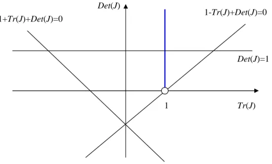
, different local dynamic results are obtainable. Figure 1 graphically represents the dynamic possibilities.

*** Figure 1 here ***

In figure 1, three bifurcation lines are represented. The space corresponding to the area inside the triangle formed by these three lines is the region of stability. Unstable outcomes are found outside the bifurcation lines. As one regards, only one kind of bifurcation is admissible in this framework, the one for which Det(J)=1, that is, a Neimark-Sacker bifurcation. The interesting point is that by introducing a slight change in a basic capital accumulation equation, regarding the amount of consumption, one generates a type of bifurcation that cannot be found in one dimensional systems. As we will observe through global dynamic analysis, invariant cycles will arise for certain values of parameters.

Proposition 3 synthesizes the result on local dynamics.

Proposition 3: The capital accumulation equation with consumption levels

adjusted to last period’s economic performance implies the following local dynamics:

a) ⋅

γ

+

δ

     + + = a a a

A 1 1 is the condition that defines the point where the

Neimark-Sacker bifurcation occurs;

b) the system is locally unstable for ⋅

γ

+

δ

     + + > a a a A 1 1 ;

c) the system is locally stable for ⋅

γ

+

δ

     + + < a a a A 1 1 .

Proof: see appendix.

Case 2: n=2. As we increase the number of periods that the representative household takes into consideration to form contemporaneous consumption decisions, the computation of a stability condition becomes harder from a calculus point of view,

but qualitatively we find that no significant changes arise: a Neimark-Sacker bifurcation continues to separate a region of stability for a relatively low technology level and a region of instability for a relatively high technology index. The analysis of this case is synthesized through proposition 4.

Proposition 4: The model of capital accumulation without optimization and with

consumption decisions based on the economic performance of the last two periods is locally characterized by the following conditions:

a) A Neimark-Sacker bifurcation exists under

δ

γ

µ

µ

µ

γ

_{+ +}         ₊ − +       ₊ ⋅ + ⋅ + = 2 2 1 2 2 ) 1 ( 1 2 a A ;

b) Local stability holds for

γ

µ

µ

µ

+

γ

+

δ

        ₊ − +       + ⋅ + ⋅ + < 2 2 1 2 2 ) 1 ( 1 2 a A ;

c) Local instability holds for

γ

µ

µ

µ

+

γ

+

δ

        ₊ − +       + ⋅ + ⋅ + > 2 2 1 2 2 ) 1 ( 1 2 a A .

Proof: see appendix.

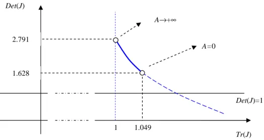
Recalling that, in our model and for n=2,

µ

+ ∑ − = × 1 ) ( ) ( M 2 J J

Det , we can clarify

the dynamics underlying this specific case by drawing a diagram that relates the sum of the order two minors of J with the determinant of the matrix. Figure 2 reveals a line segment near to the origin where stability holds, while, after the bifurcation point, instability rules.

*** Figure 2 here ***

Case 3: n=3. When consumption decisions are based on the previous three periods’ aggregate economic outcomes, the Jacobian matrix of the linearized system in the steady state vicinity will display a trace equal to 1, a positive sum of principal minors of order 1, a negative sum of principal minors of order 2, and a positive determinant. These signs lead to the unquestionable observation that two of the eigenvalues of the Jacobian matrix are negative and that the other two are positive

values. This information is vital to highlight a stability result concerning the three-period case.

Proposition 5: In the growth model without optimization, taking consumption

decisions by evaluating the previous three periods implies the following stability result. a) Local stability: 1 1 ) 1 ( 3 4 1 ) 1 ( 1 1 ) 1 ( ) 2 ( 2 2 2 4 2 3 6 <      + − − ⋅ ⋅ + + + +       + − − ⋅ ⋅       + − − +       + − − ⋅ ⋅ + + ⋅ γ δ γ µ µ µ γ δ γ µ µ µ γ δ γ µ µ µ A a A a A a and (1 )2 1

γ

µ

δ

γ

_{< +} + − − ⋅ A a ; b) Neimark-Sacker bifurcation: 1 1 ) 1 ( 3 4 1 ) 1 ( 1 1 ) 1 ( ) 2 ( 2 2 2 4 2 3 6 =      + − − ⋅ ⋅ + + + +       + − − ⋅ ⋅       + − − +       + − − ⋅ ⋅ + + ⋅ γ δ γ µ µ µ γ δ γ µ µ µ γ δ γ µ µ µ A a A a A a or (1 )2 1

γ

µ

δ

γ

_{= +} + − − ⋅ A a ; c) Local instability: 1 1 ) 1 ( 3 4 1 ) 1 ( 1 1 ) 1 ( ) 2 ( 2 2 2 4 2 3 6 >      + − − ⋅ ⋅ + + + +       + − − ⋅ ⋅       + − − +       + − − ⋅ ⋅ + + ⋅ γ δ γ µ µ µ γ δ γ µ µ µ γ δ γ µ µ µ A a A a A a or (1 )2 1

γ

µ

δ

γ

_{> +} + − − ⋅ A a .

Proof: see appendix.

To extend the analysis of local dynamics beyond n=3 is not a worthwhile task, since computation leads to heavy expressions that are progressively less informative. Nevertheless, we have found a pattern: stability holds for certain combinations of parameter values; this stability can only be broken when the product of two eigenvalues is equal to one (Neimark-Sacker bifurcation), and after the bifurcation instability will prevail (next subsection will reveal, through a numerical example, that after the bifurcation and before instability sets in it is possible that an area of quasi-periodic cycles exist).

Depending on the kind of nonlinearities involved, a bifurcation such as the one just characterized can separate regions of fixed point stability from regions of instability or it can produce a region where cycles of different periodicities emerge following the bifurcation and before instability begins to prevail. In the present model, the Neimark-Sacker bifurcation gives effectively place to endogenous fluctuations for certain combinations of parameter values. The following graphical analysis concentrates on the simplest case n=1, but since we are not limited by relevant computation problems in the numerical study of the global properties of the system, we end the section with an example that assumes n=4. We will observe that a same kind of dynamics is revealed for the two discussed cases (similar dynamics can be found for any other value of n).

Take the following set of benchmark values, which represent reasonable economic conditions (in particular, we consider a long run growth rate of 4%): [s

δ

γ

ˆy*

a]=[0.25 0.05 0.04 1 10] and let n=1. We elect A as the bifurcation parameter. In

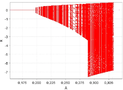
figure 3, we display the bifurcation diagram; it clearly indicates that the system undergoes a bifurcation that generates a region of cyclical behaviour for a limited interval of the parameter’s value.1

*** Figure 3 here ***

With figure 4, we take a closer look to the multiple bifurcations that this dynamic process generates, as the technology parameter is varied.

*** Figure 4 here ***

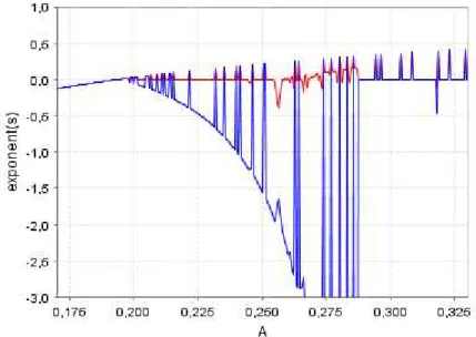
In section 2, one has discussed the possibility of the cycles arising from the bifurcation process to correspond either to quasi-periodic cycles or to chaotic motion. In particular, quasi-periodicity does not imply a divergence of nearby orbits or SDIC, and therefore one of the two Lyapunov exponents (in this case, we have an order 2 Jacobian matrix and, thus, 2 LCEs exist) can take a null value, but it will not be positive. With figure 5, that represents LCEs for different values of the index A, we clarify this point. In particular, we observe that the upper LCE is, for most of the values of the parameter, very close to zero, indicating the presence of quasi-periodicity; the jumps in the

1

All the figures concerning global dynamics presented in this paper are drawn using IDMC software (interactive Dynamical Model Calculator). This is a free software program available at www.dss.uniud.it/nonlinear, and copyright of Marji Lines and Alfredo Medio.

trajectory of both LCEs just signal small regions of instability that one can confirm to exist by looking at the bifurcation diagram in figure 3.

*** Figure 5 here ***

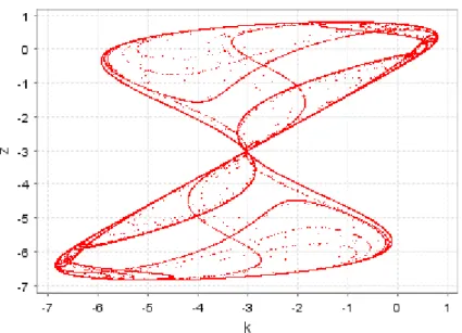
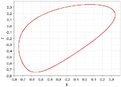
Proceeding with the visual analysis, figure 6 represents an attracting set for a value of the technology parameter with which quasi-periodicity holds, and in figure 7 a chaotic attractor is revealed, for another value of the considered parameter.

*** Figures 6 and 7 here ***

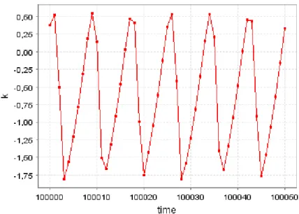
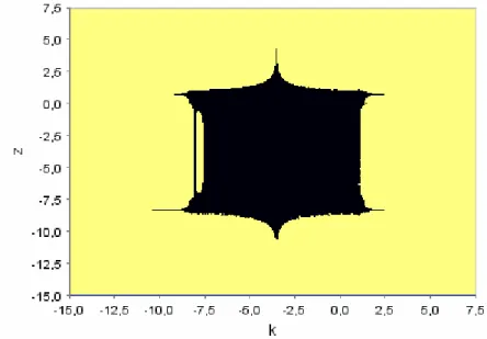
The graphical analysis becomes complete with a basin of attraction (figure 8), that we present for A=0.33, and a time series of the endogenous variable of the model (figure 9), for A=0.25. Recall that this endogenous variable, k~_t, has undertaken a double transformation: it was detrended and scaled to correspond to zero in the steady state.

*** Figures 8 and 9 here ***

With figure 9, we reveal our main result; a simple change in the conventional capital accumulation equation, that involves taking into account considerations about the business cycle when consumption decisions are made, results in endogenous business cycles. It is, as expressed in the introduction, the behaviour of households and their confidence regarding the short run economic scenario that generates and sustains economic fluctuations over time.

Note, as well, that the steady state value of the per capita physical capital variable, when the growth of trend is withdrawn, is, for the considered set of parameters,

1 . 0 75 . 0 09 . 0 1       ₋ ⋅ = A A A

k . Consider one of the assumed technology values, e.g. A=0.25;

with this value, k =5.238. Thus, the true capital variable is given by

t t

t k

k =(~ +5.238)⋅(1.04) , and its growth rate is

γ

(kt)=

(

(

k~t +5.238

) (

k~t−1 +5.238

)

)

−1.

constant, but unlike the standard endogenous growth model deterministic fluctuations on the growth rate are observable.

For n>1, a similar type of analysis is possible to undertake. To save in space, we just consider n=4 and present a bifurcation diagram like the one in figure 3 (figure 10). The same array of parameters is assumed, along with

µ

=0.05. In this case, it is clear the

occurrence of the bifurcation, of the same type as in the above example, and therefore the same kind of time trajectory as in figure 9 is obtainable for variable kt

~

, when A is above 0.105.

*** Figure 10 here ***

4. The model with optimization

The model with an exogenous savings rate can easily be sophisticated in order to incorporate consumption utility maximization. Let us now define the per capita consumption variable in the following way: c_t =E_t−1c_t +c_tc.

Term Et−1ct is the level of consumption when the output gap is permanently zero,

that is, if the expected level of output coincides with the potential level, then individuals will consume an amount E_t−1c_t of final goods. To this amount of consumption we call expected consumption. In this problem, the representative agent chooses to maximize expected utility, that is, the objective function is t

t t t c E U V =

∑

⋅

β

+∞ =1 − 1 1 ( ) . Parameter

β

<1

is the discount factor; note that we consider an infinite horizon.

The other component of consumption respects to a reaction to fluctuations. As in the non optimization case, we consider that this fraction of consumption is measured as a percentage of per capita output. Letting

σ

be a positive parameter, we define

[

( ₁, ₂,..., )−1

]

⋅ ⋅ ≡ t t₋ t₋ t₋n c t y g x x x

c

σ

. Function g is the same as in the previous section. This expression indicates that if all xt-i, i=1,2,…,n are equal to zero then ctc =0, that is,

the problem becomes the standard Ramsey growth model (in this case with a constant returns production function); it is straightforward to verify that if the weighted average of x_t−1,x_t−2,...,x_t−n is positive then c_tc >0 and, also, if the weighted average of

n t t t x x x₋1, ₋2,..., ₋ is negative then <0 c t c .

Hence, the logic underlying the theoretical structure is exactly the same as in the case without optimization: households respond to previous periods’ economic performance by consuming more (expansions) or less (recessions) than they would if one considers the benchmark model that is designed only for the case where no difference between effective and potential output is taken into account.

The utility maximization model with consumers reaction to deviations of output from its trend corresponds to the maximization of V1, subject to the resource constraint

t t

t

t y c k

k₊1 = − +(1−

δ

)⋅ , with k0 given, the variable per capita consumption as defined above and E_t−1c_t a control variable.

Since the derivation of optimality conditions is standard, we neglect the details that give place to the motion of expected per capita consumption in optimal conditions, and just present this difference equation that arises from such computation:

t t t

tc A E c

E ₊₁ =

β

⋅(1+ −

δ

)⋅ ₋₁ ; because the production function is linear, the rule that defines the time path of consumption reflects the existence of a constant growth rate of this aggregate over time. Thus, contrarily to the non optimization case, now we have an explicit growth rate γ ≡β⋅(1+A−δ)−1. Note that this is the growth rate of expected consumption, but it is also the steady state growth rate of capital and output, as one easily observes through the examination of the long term condition underlying the resource constraint.

Hence, we may define

[

]

t t t A k k ) 1 ( ˆ δ β⋅ + −

≡ as a non growing variable in the steady state. We also consider the following constant values:

[

]

t A y y ) 1 ( ˆ * *

δ

β

⋅ + − ≡ and

[

]

t t t A c E c ) 1 ( ˆ 1

δ

β

⋅ + −

≡ − _{. The constant ratio}

k cˆ

will be designated by letter

ψ

, so that we present the detrended expected consumption value as cˆ=

ψ

⋅k.

Rewriting the capital accumulation equation taking in consideration the above variables and values, we get

[ ]

[

_{[ ]}

]

        ⋅ − + ⋅ ⋅ ∑ ⋅ − ⋅ − ⋅ + ⋅ − + ⋅ =

∏

= + ⋅ − + ⋅ + − = − t n i a i t t a t t k k f k f y k k f A k i n i i ˆ ) 1 ( ) ˆ ( ) ˆ ( ) ˆ / 1 ( ) ˆ ( ) 1 ( ) 1 ( 1 ˆ 1 ) 1 /( 1 ) 1 /( 1 * 1 1 1 1 δ σ ψ σ δ β µ µ (6)

Because we have transformed the consumption variable into a detrended constant, we have, as in the previous non optimization case, a one-dimensional system of the form kˆ_t+1 =h(kˆ_t,kˆ_t−1,...,kˆ_t−n). Therefore, we must use a same kind of procedure to study the dynamics associated with this model. First, we state the balanced growth path result.

Proposition 6: The utility maximization problem with consumption reaction to

short run economic conditions has a unique steady state, which is found by imposing the condition k ≡kˆ_t+1 =kˆ_t =kˆ_t−1 =...=kˆ_t−n to (6). The balanced growth level of

accumulated capital is given by

[ ] ∑     ⋅ − + − + ⋅ − ⋅ = = − + ⋅n i i a A A A A y k 1 1 ) 1 /( 1 1 * ) 1 ( ) 1 ( ˆ µ

σ

δ

σ

ψ

β

.

Proof: see appendix.

We must guarantee a positive long run capital stock and, thus, condition

A

A

δ

σ

β

ψ

<(1− )⋅(1+ − )+ must hold.

As in the non optimization case, take k~_t ≡kˆ_t −k , ~z_1,t ≡k~_t−1, ~z_2,t ≡z~_1,t−1, …,

1 , 1 , ~ ~ − − ≡ n t t n z

z , to present another version of the capital accumulation equation,

[ ] [ ]

[

]

∏

= + ⋅ + ⋅ + − = − + ⋅         ₊ ⋅ + ⋅ − + ⋅ ∑ ⋅ ⋅ − ⋅       − + ⋅ − + − + ⋅       − + ⋅ + = n i a t i a t t a t t i n i i k z y k z k k A y A A k A A k A A k 1 ) 1 /( 1 , * ) 1 /( 1 * 1 1 1 1 ) ~ ( ˆ ~ ) ~ ( ) 1 ( ) ˆ / ( ) 1 ( 1 ~ ) 1 ( 1 ~ µ µ δ β σ δ β ψ σ β β δ β σ β (7)

The system subject to analysis is now constituted by (7), ~z_1,t+1 =k~_t and

t i t i z z, 1 ~ 1, ~ − + = , i=2,…,n, with ,~,~ ,...,~ ) (0,0,0,...,0) ~ (k z1 z2 zn = . 4.1 Local dynamics

Local analysis requires the computation of the Jacobian matrix elements. The calculus of partial derivatives and corresponding evaluation in the steady state vicinity leads to the following linearized system: