Estimating the optimal market price to sell an apartment

ABREU, C. A. C. de. Estimating the optimal market price to sell an apartment. 319

apartment

Estimativa do preço ótimo de mercado para vender um

apartamento

Carlos Alexandre Camargo de Abreu

Abstract

his paper demonstrates an investment economic analysis model based on Real Option Valuation Theory applied to decision-making of individual real estate investors. The model captures the valuation of flexibilities caused by expected market trend and uncertainty and offers an optimized value for the investment opportunity. A Real Option for investment delay is used applied to the case of postponing the selling of an apartment until the

estimated “best” optimal market price and option value. Application of the model

is made using market data from three Brazilian major cities’ real estate market. As

an important finding we have the estimation of an expanded Net Present Value for the investment when apartment selling is exercised at the optimal market price defined. It is possible to use this model to forecast what would be the optimal price and moment to sell an apartment in an investor point of view.

Keywords: Real options. Uncertainty. Investment decision. Real Estate.

Resumo

Este artigo demonstra um modelo de análise econômica de investimentos baseado na Teoria das Opções Reais aplicada à tomada de decisão de investidores imobiliários individuais. O modelo captura a avaliação das flexibilidades causadas pela tendência esperada do mercado e pela incerteza dos preços e oferece um valor otimizado para a oportunidade de investimento. Uma opção real para o adiamento do investimento é considerada e aplicada ao caso de se adiar a venda de um apartamento, até que o "melhor" preço de mercado e seu valor de opção otimizado sejamatingidos. A aplicação do modelo é feita com base em dados de mercado de três grandes cidades brasileiras utilizando dados do comportamento de preços no mercado imobiliário. Como um achado importante temos a estimativa de um Valor Presente Líquido expandido para o investimento, quando a venda de apartamentos é exercida ao preço de mercado ótimo estimado. É possível usar este modelo para prever qual seria o melhor preço e momento para se vender um apartamento em do ponto de vista de um potencial investidor.

Palavras-chave: Opções reais. Incerteza. Decisão de investimento. Mercado imobiliário.

T

¹Carlos Alexandre Camargo de Abreu

¹Universidade Federal do Rio Grande do Norte Natal - RN - Brasil

Introduction

The traditional economic evaluation model based upon the discounted cash-flow, accounts for uncertainty but just by increasing the discount rate. As a result the higher the uncertainty, the lower the present value of a project. Because of the uncertainties the performance of the future rate of return of an investment may vary accordingly to potential modifications in the market environment regarding its tendency and volatility. Smit e Trigeorgis (2012) argue that decision-makers have some flexibility to choose the best moment of investment or the instant of cashing-in the profits of an asset sold in an uncertain market, and that should be evaluated in the economic analysis process. Since the uncertainty has a potential upside and the loss is limited to investment, the traditional decision-making tends to recommend suboptimal decision-rules.

The basis of real options valuation models is that a

project’s value has behaviours similar to a financial option in derivatives markets. Pindyck and Pindyck (1994), Trigeorgis (1996) and Luehrman (1998) discussed that a real project is an option of investment, not an obligation where the investment can be made at any time until its expiration. In a real option model the asset on which the option will be valued is the real investment discounted cash flows. As it happens on future markets, real options also have an exercise price representing the value that an investor has to pay, to acquire a financial option.

In the “real markets” that will be the value of

investment costs necessary to start the investment.

An individual Real Estate investment is a type of transaction where market behaviour plays an important role. The market relates to all types of uncertainties which have the potential to interfere on the properties prices at every moment. Individual apartment buyers have all types of strategies, some will buy only to live in, others will live in until prices go up and will sell it, others might rent the apartment and wait until market price appreciation to sell the property. But what is the optimal price which a Real Estate Investor should sell the property? What is the optimal value of my investment if I consider the possibility of market changes in the future, during the time horizon of my investment? A Real Option Model could be the answer. Here, the goal is to demonstrate a Decision – Making model that takes into the evaluation of an investment opportunity possible future shifts in the Real Estate Market. The model will be applied in a context of an individual buyer seeking return for his investment in a determined time horizon. Application and

model development takes into account data from apartment markets in three of the main Brazilian cities, where real estate markets have been facing great price rise thru this century.

Works in the Real Options and Real Estate areas have been made, covering a few different areas. Fortunato et al. (2008), uses a model to determine the option values for a buyer to abandon a housing unit investment considering different refund levels. Yoshimura (2007) analysed the impact of a Real Option model on the potential value aggregation related to better evaluation of real estate construction projects. Bulan, Mayer and Somerville (2009), studied the effects of uncertainty on the delay of investments real estate projects and how competition influences this relationship.

Cunningham (2006), tests the prediction of a Real Option model related to the delay of an investment in Real Estate projects due to higher market uncertainty, while Rocha et al. (2007) values managerial flexibilities identifying the optimal strategy of investment in a Real Estate project regarding the different construction phases. Blytt (2016) uses real options considering the uncertainty of the project´s ending moment, of a real estate project where the decision-maker can stop the project for some periods. Hansteen (2015) developed the real option analysis in a commercial real estate project where the uncertainty concerns are the rental rates subject to uncertain regulations. Baldi (2013) applied a Real Option model in a multi-purpose building considering timing and scaling options for the contractor. In an empirical approach Tsekrekos andKanoutos (2013) demonstrate that in the greek real estate market investments the price behaviour suggests that decision maker consider a delaying option when investing. Shi et al. (2015) follow a similar approach investigating price formation of apartments on the Chinese markets and concluding that price uncertainty has a major influence on the market prices for the apartment deals.

Methodology

Initial investment is made at the apartment buying moment with the expectation of future return from capital gain and rent flows. When market prices are optimum there is a trigger investment decision point at which selling should be considered. So, total uncertain income (V), must compensate investment (I) when decision – making for the selling is taken.

dV =α Vdt + σ V dz Eq. 1 In Equation 1, dV represents the variation of investment income due to the oscillation of apartment´s market value, αis the expected long annual trend for V, σis the fluctuation component demonstrating how market price volatility and, consequently, investment return, performs. The dz

is the Wiener increment in charge of defining the type of oscillation modeled stochastic process. The estimation of V is observed on Equation 2.

V = (Capital Gain + Rent Income) – Property Costs – Taxes Eq. 2 The model´s uncertain variable is defined by the summation of positive and negative constituents of the investment´s cash flow, where the first are potential revenues from rent, and the second are withdrawals to keep the investment. Rent incomes are the revenues received by the investor after undertaking the investment and renting the property during some of the period of this economic analysis. Let´s consider the rent period as a deterministic variable defining that the apartment will be rented with a 75% occupation rate of the total time of the investment analysis and considering as 6 years of potential cash flow. Also deterministic is the total income from rent which the estimation is shown in Equation 3. The property size is defined as the apartment´s area, in square meters. Rent price is defined as the average value for the expected future fluctuation of rent.

Rent Income = (Rent price * Property Size) * occupation rate * Total Period Eq. 3

Capital gain is the potential value which will be cashed in by the investor due to the difference between apartment´s market sales price and its capital investment amount at the time of property acquisition. The property costs are the total expenditures related to the maintenance of the apartment which is defined to be around 1% of the initial investment, in a yearly basis. Condominium costs are added to these, which are the ones related to payments for maintaining the common areas of an apartment building. These are responsibility of the renter, but since there is an estimate of a 75% occupation rate, the property owner pays these costs in 25% of the time. The last portion of total costs is the real estate broker´s

fee, which in Brazil is around 4% of the total transaction importance and is paid by the property seller. Property costs estimations are shown in Equation 4.

Property Costs = Maintenance Costs + Condominium Costs + Broker Fee Eq. 4

The last part of the determination of (V) are the taxes involved in buying and keeping an apartment in Brazil. These taxes are: a sales tax over the transference of property ownership. In this paper there is a 2% tax rate on the investment value at the real estate acquisition moment. Property tax is a city tax paid by every owner of Real Estate properties. For this simulation it is considered a rate of 1% of the property´s value. It is an annual tax defined by a city´s legislative power and the rate can vary between different cities. Completing the taxes there are other costs related to bureaucratic documents related to the transfer of ownership. Considering a type of apartment owner very common in Brazil, which is the economic agent owning one property and selling it to acquire another apartment of higher prices or just to cash in the return from investment. Income tax is excluded from the analysis. That happens because the Brazilian taxes law has a 0% tax rates for this type of strategy. Total taxes are in Equation 5.

Taxes = Sales Tax + Property Tax + Other Eq. 5

Real Option Theory uses models, when dealing with continuous time, which divides the

decision-making process in two parts: the” right now”

investment decision and a function valuing the future potential investment decisions (DIXIT; PINDYCK 1994). The decision – Maker will always be comparing the gains from investing now and the potential returns from the estimation of a continuation value, where the decision-maker delays the investment until the optimal moment when investing presents superior value if compared to the waiting option. As in Dixit and Pindyck (1994), Equation (6) demonstrates the Bellman equation, demonstrating the maximization of the investment return in every future period.

rF 𝑉,𝑡 =max 𝜋 𝑉,𝑡 + 1 𝐸 dt dF 𝑉,𝑡

Eq. 6

Equation 6 shows the return of a decision – maker if its choice is to keep the real estate investment, postponing it´s sale. The investment estimated value is the maximum between the discounted

present value “right now” and the expected

both terms together estimates the total potential expected returns for rescheduling the sell. The real option model results are totally influenced by the expectation of the market given by the second term of equation 6. An investment project can have its total value based only on the future valuation opportunities. Hirsa andNeftci (2013) and Dixit and Pindyck (1994) show details for the differential Equation (7) that is used to estimate option values is continuous time.

½ σ2V2(dF(V,t))/ dV2) +(α) V(dF (V,t)/ dt) – rF(V,t) =0 Eq. 7

where [d2 F(V)/d (V)2] is the second derivative, [d F(V)/d (V)]the first derivative, F is the option value, r is the discount rate, σ is the volatility apartment price and α is the apartment´s expected future long time based price growth trend. Solving (7) requires boundary conditions which are shown in Dixit and Pindyck (1994). The model exploits returns for investment (V). So the desired result is thegreatest potential gains from investing in the real estate prospect with an expenditure (I) which is the price at which the property was bought by the investor at its market price. The equation estimates an optimal value V and a trigger market price at which it is optimum to make the sell and get profits from the deal. The derivation of (7) turns possible the valuation of the flexibility of a decision – maker to choose the best moment to sell an asset accordingly to market price trend and potential variation.

Long Term trend and volatility are the two main input parameters in this Real Option Model. The trend is the tendency of growth or fall of market prices of the analysed property. This research considers an annualized trend rate. The estimation of this parameter is shown in Equation 8, where n is the number of observation accordingly to quantity of data, P(t) the market price evolution index for the property at time t and P(t-1) the index at a period before. The data used to estimate 𝛼the Brazilian Real Estate prices evolution Fipe – Zap index, which has been gathering data about Real Estate prices for the Brazilian major cities since 2008, for some cities and 2010 for other group of cities. Equation 9 shows how the index is estimated in a monthly basis. Fipe-Zap (2015) states that the index has a Laspeyres format, where it is the index at month t, Pt is the market

price at the present month and Pt-1 is the market

price at the month before. Using Equation 8 it is possible to get a monthly trend evolution of market prices for the whole period of analysis that was adapted to a yearly basis.

𝛼= 1𝑛 ln 𝑖(𝑡)𝑖(𝑡 −1) Eq. 8

it = it-1 * (Pt / Pt-1) Eq. 9

The volatility parameter is the model´s input data that denotes the market oscillation. The Fipe – Zap index of Equation 9 is also used for the volatility estimate. The first step is the estimation of an yearly average for the index. The second step is to calculate the estimate of the standard deviation for the same group of yearly index data. Since the standard deviation gives a number from which the group of data is varying away from its average central value, when dividing the yearly variation measure by its yearly average, the result is an annual rate from which the market price of the property is fluctuating. To get one rate value for the time horizon for this economic analysis, the yearly volatilities are used to get the whole period average value.

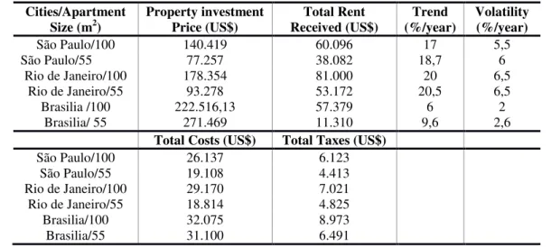
The application of the Real Option model is at the Brazilian real estate market. The data used in the analysis is from the market for medium class neighborhood apartments from three of the Brazilian major cities: Rio de Janeiro (RJ), Sao Paulo (SP) and the country´s capital, Brasilia (DF). The data gathered in Table 1 is from 3 and 2 bedroom apartments, with the first from apartments with 100 square meters and the second with 55 square meters. Table 1 also shows the rent and sales values per square meter for these type and size of apartments estimated by Fipe-Zap (2015).

Costs and taxes for the apartments analyzed are also included in Table 1. The estimation of trend and volatility parameters, used data from August 2008, the beginning of historical series for the Fipe – Zap index, until February 2014, for Rio de Janeiro and Sao Paulo Apartments market. For the Brasilia Market, data ends on February 2014 but begins at August 2010. For the case studies for 3 and 2 bedroom apartments in these cities, the supposition is that the investment in the apartment was engaged on the beginning of the series for each city, and by using the model, make the estimation of an optimal value that the investment would be maximized at which could be a moment to consider selling the apartment and cashing in the capital gains. After defining the optimum market price for selling the asset, it is used the real market prices data evolution for apartments sales at each of the cities, obtained at Fipe-Zap (2015) , during the period from 2008/2010 to 2014 to analyze what would be the decision of an investor using this model. Comparison between decision – making using Real Options and traditional NPV valuation methodology are also made.

results in decision – making, when using the Real Option model and the traditional Net Present Value financial/ economic viability indicator. There is also some discussion and comparison regarding the results in decision - making simulation concerning the different city´s markets analysed, as well as an example of the estimation of the selling moment for the apartments. All the results estimated by the real options model are based on the input data of Table 1.

Results

The first set of results from the application of the model is based on the analysis of one of the cases presented on table 1, that is, the economic viability study of investing in the acquisition of an apartment with three bedrooms and size of 100m2 at Sao Paulo. Looking at table 2 it is possible to make an examination of the NPV value for the investment. The NPV is based on the discounted cash – flow ( at a minimum attractiveness rate of return of 10%) results, for each of the 6 years of our time horizon of the study, considering all potential revenues, costs and taxes estimated for the investment.

The discounted values are added and then subtracted from the price of investing resulting in a financial importance indicating economic viability or not. The NPV decision rule indicates the decision-maker to sell the property if NPV is above zero, demonstrating some positive financial result. In this case study, after investing US$ 140.419 in the purchase the decision to sell the apartment could be taken at the moment when net

income surpassed the investment price. Focusing analysis in a US$ 45.000 interval for each decision, NPV would indicate a transaction at a total income of US$ 157.496and, consequently, a NPV of US$ 17.076. That NPV will occur with the apartment´s market price getting to around US$ 396.000. At prices below at which the returns are very low, and when market prices go below US$

225.000 the decision in “do not sell the property”,

since the NPV will be below zero, defining a financial loss.

The Real Option Model has a different decision – making rule. It is possible to observe, on table 2, that the option value only exists with a positive net income potential flow coming from expected rent revenue and possible capital gain. That is related to the basic concept of Real Options Theory which assumes an investment as an opportunity that will be taken only if market conditions are favourable.

If apartment’s prices are under, approximately

US$ 112.500, there will not be any positive net income as observable on table 2, when the market prices are US$ 90.000 and US$ 45.000. In these market situations the value of the apartment selling opportunity is zero, since there is no expected positive cash flow from selling the property at that price. When we have a US$ 135.000 projected market price the option value for the investment is slightly positive. From that market price level the opportunity of selling the apartment has some value. With market prices from around US$ 112.500 to nearby US$ 253.500, where NPV gets positive, we have an option value for the investment but a negative NPV.

Table 1– Real Options Model Data

Cities/Apartment

Size (m2₎ Property investment _{Price (US$) Received (US$)}Total Rent _(%/year)Trend Volatility _(%/year)

São Paulo/100 140.419 60.096 17 5,5

São Paulo/55 77.257 38.082 18,7 6

Rio de Janeiro/100 178.354 81.000 20 6,5

Rio de Janeiro/55 93.278 53.172 20,5 6,5

Brasilia /100 222.516,13 57.379 6 2

Brasilia/ 55 271.469 11.310 9,6 2,6

Total Costs (US$) Total Taxes (US$)

São Paulo/100 26.137 6.123

São Paulo/55 19.108 4.413

Rio de Janeiro/100 29.170 7.021

Rio de Janeiro/55 18.814 4.825

Brasilia/100 32.075 8.973

Despite the negative net inflow of cash the Real Option, at that interval, is positive due to the expectation that prices will rise, in reason of an expected growth tendency (17% each year) and an expected volatility (5,5% yearly) that might make the apartment prices have an upper fluctuation. In case of negative variation the decision-maker will not sell the apartment. Also in the reason of these expectations, related to market price behaviour, we

have a Real Option decision rule of “wait to sell

the property”, at market price interval between US$253.500 and US$ 396.000. At that same price

range the NPV decision rule is “Sell the property and cash in the capital gains”.

The dissimilarity in decision rules is exactly because of the expectations regarding property

prices evolution. The trigger “sell the property point” will occur after waiting for market

oscillation, when prices reach US$396.000. At that price NPV and Option values are the same, representing the optimal investment moment, from where the effects of minimal future expectations have been incorporated to the opportunity value. This is a threshold investing value.

If owner´s interest is to wait even more, that is a valid decision, but there will not be any other point indicating investment. Prices above US$ 396.000

have a “take the investment” decision accordingly

to the Real Options Model.

Table 3 shows a comparison of the option to invest optimal value, its optimal market price, the market price that would trigger the investment with NPV rule and investment/Trend/Volatility for each case. Comparing the apartments price in Rio de Janeiro and Sao Paulo it is to possible to observe that the option value for the optimum investment are superior in the first city. The main reason is the slightly higher trend and volatility parameters. The

“waiting” option to sell the apartment has a greater value in Rio´s markets because the expectation of yearly growth in prices are 3% (bigger apartment) and 1.8% (smaller properties). If the investor thinks the market prices will evolve more in Rio,

the “waiting” decision will be more valued. If

markets in Rio have a superior oscillation, the investor´s decision to wait will also have a superior value, since the expected price´s positive oscillation has a potential of greater upper swings then in Sao Paulo. Another reason for the difference in option values between both cities is, the investment price that is 27% higher for big apartments and 21% in the smaller type.

Greater property investments cashed out by the owners means higher needs of capital gains at the selling moment assuring the investment´s financial return. So, the waiting option value will grow

since the investor has the necessity of postponement of the selling moment to get a potential higher income. Comparing both of these cities to Brasilia, there is a much higher option value for the last market. That happens because of the much higher apartment prices at the buying moment by the investor. The differences in prices are so high that the waiting option is very appreciated. The lower trend and volatility have little influence in reducing the value of waiting due to the extreme initial investment. Therefore, Brasilia has the greatest optimal selling prices. The average difference between optimal prices, using the model and with the NPV decision rules (trigger point above zero) is of 52%. So, it seems to be a strategic move for the investor, waiting for the best moment to invest indicated by the Real Option Model.

The model can be used to forecast an optimal point in time estimating the selling transaction date. That can happen if the decision-maker has data related to yearly or monthly predictions of price evolution. The procedure is to compare the periodic price forecast to the model´s indication of optimal market prices, which would generate the optimum option value To exemplify that let´s suppose that the investor bought the apartment at the investment initial price (I) at August 2008, for the cities of Rio and São Paulo and June 2010 for Brasilia´s apartments. That date is the beginning of the

public time series for the index and it’s per square

meter prices for apartments in Brazilian major cities. The real market data is followed until February 2014.

So, it is possible to compare the optimal option value and the property market price that will trigger it to the real market data between 2008/2010 until 2014, and look at what date the market prices reached the model´s decision rule

(June 2010) and the very small growth in prices, showed in its trend.

The Brasilia Market from Base date until February 2014 progressed only 24%. So, that supposed investor from Brasilia, probably missed the buying moment for apartment investment, unlike investor

from the other two cities, accordingly to the analysis with the Real Options Model. Using the case S. Paulo/ 100 it is possible to make a sensitivity analysis of the main variables influencing on the models essential result regarding the optimized market price of selling.

Table 2– NPV and Option Value (Case: São Paulo 100 m2₎ Capital

Gain (US$)

Rent Income

(US$)

Costs (US$)

Taxes (US$)

Net Income

(US$)

Investment (US$)

NPV (US$)

Option (US$)

Market Value (US$)

(95.419) 60.097 26.139 6.043 (67.504) (140.419) (207.924) - 45.000 (50.419) 60.097 26.139 6.043 (22.504) (140.419) (162.924) - 90.000 (5.419) 60.097 26.139 6.043 22.496 (140.419) (117.924) 941 135.000 39.581 60.097 26.139 6.043 67.496 (140.419) (72.924) 8.314 180.000 84.581 60.097 26.139 6.043 112.496 (140.419) (27.924) 22.893 225.000 129.581 60.097 26.139 6.043 157.496 (140.419) 17.076 44.611 270.000 174.581 60.097 26.139 6.043 202.496 (140.419) 62.076 73.424 315.000 219.581 60.097 26.139 6.043 247.496 (140.419) 107.076 109.303 360.000 255.581 60.097 26.139 6.043 283.496 (140.419) 143.076 143.076 396.000 309.581 60.097 26.139 6.043 337.496 (140.419) 197.076 202.162 450.000 354.581 60.097 26.139 6.043 382.496 (140.419) 242.076 259.104 495.000 399.581 60.097 26.139 6.043 427.496 (140.419) 287.076 323.033 540.000 444.581 60.097 26.139 6.043 472.496 (140.419) 332.076 393.936 585.000

Table 3– Cities Results

Cities/Apartment Size (m2₎

Property investment Price

(US$) Trend (%/year) Volatility (%/year)

S. Paulo/100 140.419 17 5,5

S. Paulo/55 77.257 18,7 6

Rio/100 178.354 20 6,5

Rio/55 93.277 20,5 6,5

Brasilia/100 271.469 6 2

Brasilia/55 175.326 9,6 2,6

Option Value

(US$) Optimal Market Price - Options (US$) Price - NPV (US$) Optimal Market

S. Paulo 100 143.076 396.000 253.500

S. Paulo/55 79.045 219.000 141.000

Rio/100 181.596 493.500 312.000

Rio/55 94.974 252.000 157.500

Brasilia/100 272.660 838.140 566.080

Brasilia/55 176.946 553.880 376.980

Table 4 – Model´s Selling Moment

Cities/Apartment

Size (m2₎ Optimal Market _{Price (US$)} Selling Moment Total Period _(Years)

S. Paulo/100 396.000 February 2014 5,5

S. Paulo/55 219.000 October 2013 5,2

Rio/100 493.500 December 2012 4,3

Rio/55 252.000 June 2012 3,9

Brasilia/100 838.140 Wait -

Conclusions

The decision-rule using the model is sensitive to price uncertainty, market trend and the apartment initial value. The greater expected price growth tendency the sooner the optimal price for the selling decision. Real option models are valuable tools to be used in economic evaluation of individual Real Estate investment opportunities especially on environments with a price growth expectation and potential capital gains. Different city or market scenarios will change the investment decision due to unequal estimates of market conditions. Higher level of uncertainty delays the option to sell, but in the cases studied there were not very elevated degrees of uncertainty. The tool allows a decision-maker to measure economic impacts on the opportunity of investment´s value, coming from probabilistic gains from the existence of possible positive future market expectations. The quantification of this flexibility on waiting for better conditions to sell is the key aspect of this model.

A real option approach in the decision – making in the demand side of the market is also important since the decision to invest is totally affected by the uncertainties in apartment prices. So, models based on this theory can also be used for “smaller” everyday traditional investors or even in the financial decision in families.

References

BALDI, F. Valuing a Greenfield Real Estate Property Development Project: a real options approach. Journal of European Real Estate

Research, v. 6, n. 2, p. 186-217, 2013. BLYTT, K. Uncertainty in Real Estate

Development. 2016. Doctoral Thesis. Norwegian School of Economics.

BULAN, L.; MAYER, C.; SOMERVILLE, C. T. Irreversible Investment, Real Options, and Competition: evidence from real estate

development.Journal of Urban Economics, v. 65, n. 3, p. 237-251, 2009.

CUNNINGHAM, C. R. House Price Uncertainty, Timing of Development, and Vacant Land Prices: evidence for real options in Seattle. Journal of

Urban Economics, v. 59, n. 1, p. 1-31, 2006.

DIXIT, A. K.; PINDYCK, R. S.Investment

Under Uncertainty. Princenton: Princeton University press, 1994.

FIPE ZAP. Índice FIPE ZAP de Preços de

Imóveis Anunciados. Disponível em:

<http://www.fipe.org.br/pt-br/indices/fipezap/

>

FORTUNATO, G. et al.Valor da Opҁão de

Abandono em Lanҁamentos Imobiliários

Residenciais. RAC - Eletrônica, v.2, n. 3, p. 531-545, 2008.

HANSTEEN, J. The Value of Expanding

Commercial Rental Space. Oslo, 2015. Doctoral Thesis, Norwegian School of Economics, 2015.

HIRSA, A.; NEFTCI, S. N. An Introduction to

the Mathematics of Financial Derivatives. London: Academic Press, 2013.

LUEHRMAN, T. A. Investment Opportunities as Real Options: getting started on the numbers.

Harvard Business Review, v. 76, p. 51-66, 1998. MCDONALD, R.; SIEGEL, D. The Value of Waiting to Invest. The Quarterly Journal of

Economics, v. 101, n. 4, p. 707-727, 1986. ROCHA, K. et al. Real Estate and Real Options: a case study. Emerging Markets Review, v. 8, n. 1, p. 67-79, 2007.

SHI, S. et al. Uncertainty and New Apartment Price Setting: a real options approach.

Pacific-Basin Finance Journal, v. 35, p. 574-591, 2015. SMIT, H.; TRIGEORGIS, L. Strategic

Investment: real options and games. Princenton: Princeton University Press, 2012.

TRIGEORGIS, L. Real Options: managerial flexibility and strategy in resource allocation. Cambridge: MIT press, 1996.

TSEKREKOS, A.Ε.; KANOUTOS, G. Real Options Premia Implied From Recent Transactions in the Greek Real Estate Market. The Journal of

Real Estate Finance and Economics, v. 47, n. 1, p. 152-168, 2013.

Carlos Alexandre Camargo de Abreu

Escola de Ciências e Tecnologia | Universidade Federal do Rio Grande do Norte | Campus Universitário, Sala 54, Lagoa Nova | Natal - RN – Brasil | CEP 59014-615 | Tel.: (84) 99444-7498 | E-mail: calexandreabreu@ect.ufrn.br

Revista Ambiente Construído

Associação Nacional de Tecnologia do Ambiente Construído Av. Osvaldo Aranha, 99 - 3º andar, Centro

Porto Alegre – RS - Brasil CEP 90035-190 Telefone: +55 (51) 3308-4084

Fax: +55 (51) 3308-4054 www.seer.ufrgs.br/ambienteconstruido

E-mail: ambienteconstruido@ufrgs.br