Ecologia e Conservação de Recursos Naturais
Efeitos de reservatórios artificiais
sobre a composição florística e a estrutura de
comunidades arbóreas nativas no Triângulo Mineiro
Vagner Santiago do Vale
Ivan Schiavini
(Orientador)
Efeitos de reservatórios artificiais
sobre a composição florística e a estrutura de
comunidades arbóreas nativas no Triângulo Mineiro
Orientador
Prof. Dr. Ivan Schiavini
Uberlândia - MG
Fevereiro/2012
Dados Internacionais de Catalogação na Publicação (CIP) Sistema de Bibliotecas da UFU, MG, Brasil.
V149e 2012
Vale, Vagner Santiago do, 1983-
Efeitos de reservatórios artificiais sobre a composição florística e a estrutura de comunidades arbóreas nativas no Triângulo Mineiro / Vagner Santiago do Vale. -- 2012.
167 f. : il.
Orientador: Ivan Schiavini.
Tese (doutorado) - Universidade Federal de Uberlândia, Programa de Pós-Graduação em Ecologia e Conservação de Recursos Naturais. Inclui bibliografia.
1. Ecologia - Teses. 2. Represas - Aspectos ambientais - Teses. 3. Solos - Umidade - Teses. 4. Impacto ambiental - Avaliação - Teses. 5. Flora dos cerrados - Triângulo Mineiro (MG) - Teses. I. Schiavini, Ivan. II. Universidade Federal de Uberlândia. Programa de Pós-Graduação em Ecologia e Conservação de Recursos Naturais. III. Título.
CDU: 574
Vagner Santiago do Vale
Efeitos de reservatórios artificiais sobre a composição
florística e a estrutura de comunidades arbóreas nativas no
Triângulo Mineiro
____________________________
Prof. Dr. Fabrício Alvim Carvalho
Instituto de Ciências Biológicas e Geociências – UFJF ____________________________
Prof. Dr. Frederico Augusto Guimarães Guilherme Centro de Ciências Agrárias – UFG
____________________________ Prof. Dr. Glein Monteiro de Araújo Instituto de Biologia – UFU
____________________________ Prof. Dr. André R. Terra Nascimento Instituto de Biologia – UFU
____________________________ Prof. Dr. Ivan Schiavini
Instituto de Biologia – UFU (Orientador)
Uberlândia – MG
Fevereiro/2012
Dedico...
Aos integrantes do Laboratório de
Ecologia Vegetal:
Ivan, Sérgio, Ana,
Jamir, Carol, Maca, Glein
e á minha
família francana:
Pai, Mãe, Vi,
Várias pessoas têm minha gratidão, não só pelos quatro anos de doutorado, mas desde muito
antes. Desde os tempos da graduação tenho contado com a orientação e apoio do professor Ivan, sempre
dando dicas, pitacos e jogando idéias interessantes para serem estudadas. Valeu mesmo o convite pro
doutorado e tentei atender as espectativas. Bom, acho que melhorei bastante e parte desse crescimento
científico se deve à sua orientação.
Outro que ajudou demais, e ajudou muito, foi o professor Glein. Ele e o Ivan foram os mentores do
projeto quando ele nasceu e como se não bastasse, foram para vários e vários campos. O Glein conhece
bem o projeto e sabe o quão pesado foi o serviço. Espero ter correspondido na escrita da tese, e saiba que
aprendi bastante com você nos vários campos que fizemos.
Vou agradecer algumas intituições, direcionando áqueles que se dedicam e levam a sério o serviço.
Obrigado UFU pelo ensino, á Pós Graduação em Ecologia e Conservação de Recursos Naturais pelo suporte
acadêmico e a FAPEMIG e CAPES pelo suporte financeiro para minha pesquisa. Também volto a Agradecer
á Pós Graduação em Ecologia (Maria Angélica e colegiado) e a FAPEMIG (além dos professores que dedicam
tempo para realizar o pedido de auxílios nos congressos) pelo apoio para a divulgação de trabalhos em
congressos, e de novo a UFU pelo transporte aos congressos.
Agradeço demais, e demais messsssssmo a famigerada galera do LEVe, pra quem não conhece é o
Laboratório de Ecologia Vegetal da UFU. Espero um dia poder criar um laboratório semelhante. O ambiente
de trabalho é excelente, galera trocando idéias e se ajudando para melhorar não só a qualidade dos
trabalhos como também da nossa própria vida. Quem fica ali e se estabelece, é pela competência
dedicação e companheirismo, por isso admiro cada um de vocês e espero manter contatos quando a vida
nos encaminhar para faculdades diferentes. Mais que colegas, considero todos vocês meus amigos,
obrigado por todos os momentos marcantes, felizes, picuinhas e divertimentos. Nominalmente, ao Sérgio
(ex-chefe) fica a certeza que perseverar vale a pena, a Ana (ex-Paulão) fica as intermináveis análises
estatísticas que aprendi e a tranqüilidade dos bons ventos que virão e ao Maca (ex-André) obrigado pelo
solo coletado e idéias pra escrever. Vocês estão na vibe aí comigo a muito tempo, obrigado muito,
principalmente pela paciência por me tolerar por tantos anos.
Aos novos doutores, Jamir e Carol, espero que esses dois últimos anos tenham sido proveitosos pra
vocês da mesma forma que foi pra mim. Compartilhamos tabelas, fios brancos, leituras e estatísticas. Valeu
mesmo!!! Ver voces no mestrado, ralando bastante pra terminar os trabalhos me deu um gás extra e
motivação para fazer um bom doutorado. Obrigado também aos insipientes da graduação pela ajuda no
voltaram – obs, se eu me esqueci de alguém, foi MAL AE!!!) e aos sumidos Olavo e Pedro Paulo, que
sempre animam o ambiente com suas visitas esporádicas, abusando dos trocadilhos infames, e á Simone
Mendes por sempre ser solícita em fornecer informações sobre as usinas hidrelétricas em que trabalhei.
Bom, acho que agradeci a metade da galera que me apoiou. A outra metade está lá na minha
terrinha... lá na Franca. Pai (Paulo Roberto do Vale), e Mãe (Maria de Lourdes Santiago do Vale) esta tese é
só mais um dos muitos fruto cultivados por vocês. Vocês são a condição sine qua non para minhas vitórias, por sempre me apoiarem nas minhas escolhas e em momento algum duvidar da minha capacidade. Isso
sem falar na educação que me deram e na extrema paciência com o filho mais enjoado que tiveram.
Brigadão Viviane, minha irmã mais velha que amo de paixão. Vou sempre procurar estar perto de
você pra dar amor, apoio e carinho, porque é justamento o que você sempre me ofereceu. A minha
“irmãzinha cotoquinho lindo” preciso nem agradecer nada não. Tenho é que me orgulhar, apesar de
sempre se encrencar com a mãe, está virando um mulherão. Espero que siga o exemplo do seu irmão e
procure fazer o que gosta, para poder ser feliz na vida e na profissão. Bom, o irmão e seu exemplo maior
que estou falando é o Vandão claro!!! Esse sim vai ser sempre meu ídolo, sempre a pessoa que vou me
comparar para continuar melhorando. Aprendi demais contigo brother!!! Brigadaço!!!
Por fim, tenho que agradecer á minha namorada por me agüentar e sempre fazer eu voltar pra
Uber feliz (neh danada!?), ao meu vééélho amigo Diego pelos jogos e histórias que vão virar lenda a
toooda família de Franca, lá do Goiás e por aí afora.
Obrigado! Obrigado mesmo!
Lista de Figuras ... 4
Lista de Apêndices ... 7
Introdução Geral ... 9
Chapter 1: Efeitos no curto prazo da redução do fluxo de água em comunidades florestais ciliares 11 Resumo ... 12
Introdução ... 13
Material e Métodos ... 15
Resultados ... 18
Discussão ... 29
Apêndices ... 34
Capítulo 2: Grupos de dinâmica e heterogeneidade de uma floresta ciliar: distintas respostas após redução na vazão de água de um rio 35 Resumo ... 36
Introdução ... 37
Material e Métodos ... 39
Resultados ... 42
Discussão ... 52
Apêndices ... 56
Capítulo 3: Alterações na comunidade de florestas sazonais sob impactos de barragem: um estudo de dinâmica 59 Resumo ... 60
Introdução ... 61
Material e Métodos ... 62
Resultados ... 65
Discussão ... 71
Apêndices ... 76
Capítulo 4: Mudanças rápidas na composição e na diversidade: consequências das represas para as florestas secas estacionais. 82 Resumo ... 83
Introdução ... 84
Material e Métodos ... 85
Resultados ... 88
Discussão ... 102
Conclusão ... 109
Apêndices ... 110
Capítulo 5: Grupos de resposta dinâmica de espécies devido aos impactos de reservatórios nas florestas: um contraste entre ambientes sazonais 124 Resumo ... 125
Introdução ... 126
Material e Métodos ... 127
Resultados ... 130
Discussão ... 138
Considerações finais ... 144
Lista de Tabelas
Chapter 1: Pag
Table 1.1 - Wilcoxon test results (with “p “and “Z” values) for soil moisture in each season between different soil depths. MR = middle rainy season, ER = end rainy season, MD = middle dry season, ED = end dry season, T0 = before spillway construction, T1 = one year after and T3 = three years after flow reduction in a riparian forest in southern Brazil. In bold p < 0.05 and in italic p < 0.10.
-19
Table 1.2 - Diversity indexes (with respective tests results) and evenness for number of individuals and basal area in a riparian forest in southern Brazil. Different letters indicate significant variation between times.
-20
Table 1.3 - Wilcoxon test between basal areas in the plots in T0, T2, T4 in a riparian forest in southern Brazil. In bold p < 0.05 and in italic p < 0.10. -21 Table 1.4 - Dynamics parameters in four years of water flow reduction in a riparian forest
in southern Brazil.
-21
Table 1.5 - Species dynamic rates between T0 – T4 in descending order of Overall net change (ChN+ChAB)/2) to species with 10 or more individuals. M = mortality rate, O = outgrowth rate, R = recruitment rate, I = ingrowth rate, TN = individuals turnover, TBA = basal area turnover, ChN = individuals net chance, ChBA = basal area net change, ONC = overall net change; U = understory, I = intermediary, C = canopy (*Rodrigues et al 2010 classification) in a riparian forest in southern Brazil.
-26
Chapter 2:
Table 2.1 - Friedman test before, one year and three year after dam construction to 0 – 10 cm, 20 – 30 cm and 40 – 50 cm deep near and far the shore in a Riparian Forest in southern Brazil. In bold, p < 0.05. In bold p < 0.05 and in italic p < 0.10.
-43
Table 2.2 - Wilcoxon test in three depths between near and distant to the shore for four season in a riparian forest in southern Brazil. In bold, p < 0.05. MR = middle of rainy season, ER = end of rainy season, MD = middle of dry season, ED = end of dry season. In bold p < 0.05 and in italic p < 0.10. Median on Appendix 2.
-43
Table 2.3 - Genenal changes and dynamics in riverside, stream and distant sectors four years after river reduction flow in a riparian forest in southern Brazil.
-45
Table 2.4 - Kruskall Wallis test and median test (p\Z values) comparing riparian sectors before spillway construction (T0) and four years after water flow reduction (T4), in a riparian forest in southern Brazil. In bold, p < 0.05. BA = basal area.
-46
Table 2.5 - Morisita-Horn similarity in riparian sectors (riverside, stream and distant) before water flow reduction (T0), four years after flow reduction (T4), dead trees and recruits, in a riparian forest in southern Brazil. In bold p < 0.05 and in italic p < 0.10.
-46
Table 2.6 - Wilcoxon comparing changes during T0 – T4 in riverside, stream and distant sectors plots, in a riparian forest in southern Brazil. In bold p < 0.05 and in italic p < 0.10.
Table 2.7 - Discriminant Function Analysis Summary to four rates in a riparian forest in southern Brazil. Wilks' Lambda: 0.05; F (12,111) = 19.289 p<0.001. In bold p < 0.05 and in italic p < 0.10.
-49
Table 2.8 - Coherence between cluster groups and discriminant analysis groups in a
riparian forest in southern Brazil. -49
Table 2.9 - Discriminant function analysis summary to two first discriminant roots in a riparian forest in southern Brazil. In bold p < 0.05 and in italic p < 0.10.
-49
Table 2.10 - Dinamics rates for “dynamics groups” in four years of water flow reduction in a riparian forest in southern Brazil. Ni = number of individuals, BA = basal area, Mort = mortality, Recr = recruitment, TN = individuals turnover, TAB = basal area turnover, ChN = individuals net change, ChBA = basal area net change and ONC = overall net change.
-50
Table 2.11 - Density and Basal area to four dynamics groups found in cluster and discriminant analisys in three riparian sectors, in a riparian forest in southern Brazil.
-51
Table 2.12 Wilcoxon test to number of individuals and basal área among dynamics groups in each riparian sector to a riparian forest in southern Brazil. In bold, p < 0.05.
-51
Chapter 3:
Table 3.1 - Tree community parameters on three measurement times, before damming (T0), two (T2) and four years (T4) after damming and tree community dynamics between measurement times (T0 to T2, T2 to T4 and T0 to T4 periods). DF1 = Deciduous Forest 1, DF2 = Decidudous Forest 2 and SF = Semideciduous Forest.
-68
Table 3.2 - Analysis of variance (ANOVA) to number of individuals and basal area between three measurement times (T0, T2 and T4), to three Dry Forest on southern Brazil. In bold p < 0.05.
-69
Table 3.3 - Paired “t” test to number of individuals and basal area among T0-T2 and T2-T4 period to three Dry Forests on southern Brazil. In bold p < 0.05 and in italic p < 0.10.
-70
Table 3.4 - Paired “t” test among plots close to the lakeshore (0-30 m) and plots distant to margin (30-60 m) to number of individuals and basal area to all periods (T0-T2, T2-T4 and T0-T4) in three Dry Forest on southern Brazil. In bold p < 0.05 and in italic p < 0.10.
-71
Chapter 4:
Table 4.1 - Number of species and diversity Shannon index to three dry forest before (T0), two (T2) and four years (T4) after dam construction in southeastern Brazil. Letters refers to Hutcheson t test, same letters means same diversity, degree of freedom > 500, p < 0.05.
-89
Table 4.2 - Tree species parameters and dynamic rates to a Deciduous Forest (Deciduous Forest 1 – DF1) in southearn Brazil. T0 = before dam construction, T2 = two years after damming, T4 = four years after damming, M = mortality, R = recruitment, O = outgrowth, I = ingrowth.
Table 4.3 - Tree species parameters and dynamic rates to a Deciduous Forest (Deciduous Forest 2) in southearn Brazil. T0 = before dam construction, T2 = two years after damming, T4 = four years after damming, M = mortality, R = recruitment, O = outgrowth, I = ingrowth. Only species with at least 20 individuals are shown.
-93
Table 4.4 - Tree species parameters and dynamic rates to a Semideciduous Forest (SF) in southearn Brazil. T0 = before dam construction, T2 = two years after damming, T4 = four years after damming, M = mortality, R = recruitment, O = outgrowth, I = ingrowth. Only species with at least 20 individuals are shown.
-94
Table 4.5 - Tree species turnover and net change to a Deciduous Forest (Deciduous Forest 1 - DF1) by descending order of overall net change in T0-T4 period, in southeastern Brazil. Ind = individuals, BA = Basal area. Only species with at least 20 individuals are shown.
-99
Table 4.6 - Tree species turnover and net change to a Deciduous Forest (Deciduous Forest 2 – DF2) by descending order of overall net change in T0-T4 period, in southeastern Brazil. Ind = individuals, BA = Basal area. Only species with at least 20 individuals are shown.
-100
Table 4.7 - Tree species turnover and net change to a Semideciduous Forest (SF) by descending order of overall net change in T0-T4 period, in southeastern Brazil. Ind = individuals, BA = Basal area. Only species with at least 20 individuals are shown.
-101
Chapter 5:
Table 5.1 - Discriminant Function Analysis Summary to four groups in deciduous forests in southern Brazil. In bold, p < 0.05, and in italic p < 0.10.
-133
Table 5.2 - Discriminant function analysis summary to two first discriminant roots in a riparian forest in southern Brazil. In bold, p < 0.05. -133 Table 5.3 - Discriminant Function Analysis Summary to four groups in semideciduous
forests in southern Brazil. . In bold, p < 0.05.
-133
Table 5.4 - Discriminant function analysis summary to two first discriminant roots in a semidediduous forest in southern Brazil. . In bold, p < 0.05. -134 Table 5.5 - Dynamics rates for “dynamic groups” for deciduous and semideciduous
forests in southern Brazil. Control refers to forest sites not affected by dam, T0-T2 refers to forest sites in the first two years after dam construction and T2-T4 refers to the next two years after damming. M = mortality, R = recruitment, O = outgrowth, I = Ingrowth, Ind = individuals, BA = basal area, ONC = overall net change, * = group with just a species.
Lista de Figuras
Chapter 1: Pag
Figure 1.1 - Study area image marked with a square showing studied area. A = Spillway and the beginning of Reduced Outflow Stretch, A’ = end of Reduced Outflow Stretch, B = hydroelectric dam, B’ = end of hydroelectric dam, C = artificial lake created by dam, D = river patch returns to normal flow.
-15
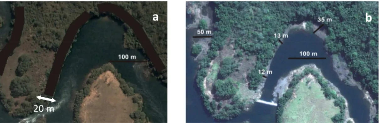
Figure 1.2 - Satellite image of riparian forest, object of this study, a = 2005 (T0) riparian plots figure and b = 2009 (T4) riparian forest showing flow reduction and the distance between forest with water after spillway construction. Plant sample were plotted along the black belt (a).
-15
Figure 1.3 - Box-Plot representation to Kruskall-Wallis test to distinct depths before spillway construction (T0), one year after (T1) and three years after flow reduction (T3) in a riparian forest in southern Brazil. Dashes = range, Bars = interval between first and third quartile, square = median. Results detail on Appendix 1.
-22
Figure 1.4 - Comparison of mortality/recruitment rates (A) and outgrowth/ingrowth rates (B) in species with 10 or more individuals in a riparian forest in southern Brazil. Square = community net change, triangles = species with positive individuals net changes, circles = species with negative individuals net changes, blue diamond = species with individual net changes lower than community and black diamond = species with individuals net changes lower than community but with area basal net change higher than community. Species Legend in Table 5.
-23
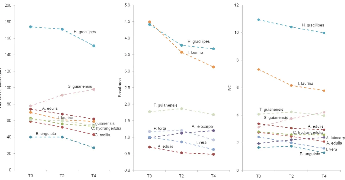
Figure 1.5 - Number of individuals, basal area and cover value to non-stable species in a Riparian Forest in southern Brazil, only those with 10 or more individuals (see figure 4A and 4B) and only those species that represents most changes in the arboreal community.
-28
Chapter 2:
Figure 2.1 - “1A” Study area image with square showing plots locations. A = Spillway and the beginning of Reduced Outflow Stretch, A’ = end of Reduced Outflow Stretch, B = hydroeletric dam, B’ = end of hydroelectric dam, C = artificial lake created by dam, D = river patch returns to normal flow. The square ilustrates the study area. “1B” Riparian forest sectors: stream (red), riverside (blue) and distant to the shore (black) plots. Plots were allocated along the tracks.
-40
Figure 2.2 - DCA analysis based in species density per plot, among riparian plots in southern Brazil. Blue circles are plots near to the shore, black circles are plots distant to the shore and red circles are plots near a stream. Schematic representation is presented in Figure 1b.
-44
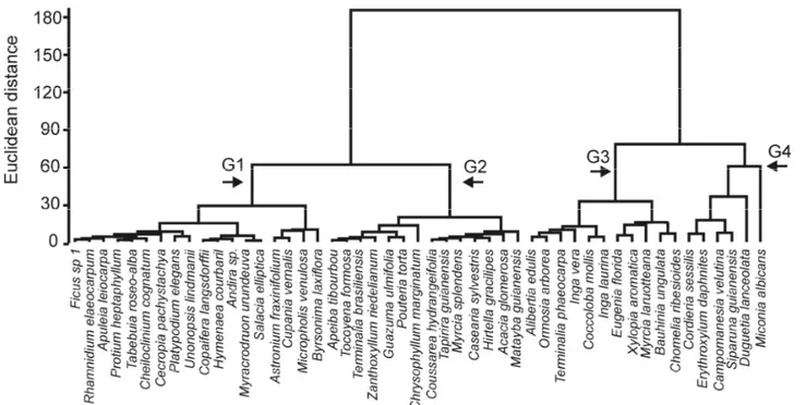
Figure 2.3 - Cluster analysis using Euclidian distance and ward method. Groups were formed based in species annual dynamic rates (mortality, recruitment, outgrowth and ingrowth), in a riparian in southern Brazil. G1 = group 1; G2 = group 2; G3 = group 3 and G4 = group 4.
-48
Figure 2.4 - Discriminant analysis based in species annual dynamic rates (mortality, recruitment, outgrowth and ingrowth) in a riparian forest in southern Brazil. Black triangle = group 1, Brown diamond = group 2, Blue circles = group 3;
Green square = group 4; * = Cordieria sessisis (discriminant analysis changes this species from G4 to G1) and ** = Bauhinia ungulate (discriminant analysis changes this species from G3 to G2).
Chapter 3:
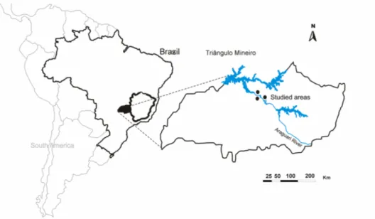
Figure 3.1 - Location of three Dry Forest which were affected by Amador Aguiar Complex Dam, on Triângulo Mineiro, southern Brazil. Before dam construction these forests were distant from water sources and now are on the artificial lake margin.
-63
Figure 3.2 - “A” - Representation of upstream landscape changes and water proximity to Dry Forest after dam construction. “B” - Plots scheme used to arboreal community samples in three Dry Forests.
-63
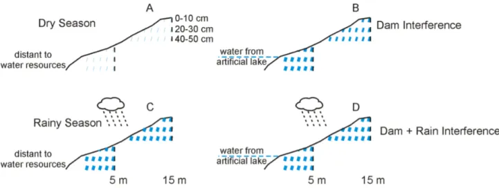
Figure 3.3 - Summary of soil moisture changes occurred due construction of dams. A and C represents soil moisture on dry forests before damming and B and D represents soil moisture after damming construction. A B shows high damming influences to soil moisture on dry season; the soil moisture increase after dams construction breaking the strength of dry season. C D show low damming influences to soil moisture on rainy season; the increase in soil moisture was less conclusive due rainfall variation in these periods. The continuous line represents soil surface, vertical black bars represents soil samples sites, blue bars represents soil moisture and their thickness illustrates soil moisture, then thicker bars represents more water available on soil; 5m and 15m represents the distance to the lakeshore after damming. After dam influence, soil moisture increase mainly on dry season and mainly near to the lakeshore. Soil moisture details were summarized on Appendix 4,5,6,7,8 and 9.
-66
Chapter 4:
Figure 4.1 - Location of three Dry Forest which were affected by Amador Aguiar Complex Dam, on Triângulo Mineiro, southern Brazil. Before dam construction these forests were distant from water sources and now are on the artificial lake margin.
-86
Figure 4.2 - “A” - Representation of upstream landscape changes and water proximity to Dry Forest after dam construction. “B” - Plots scheme used to arboreal community samples in three Dry Forests.
-86
Figure 4.3 - Comparison of recruitment/mortality (A and C) and ingrowth/outgrowth rates (B and D) in species with 20 or more individuals in Dry Forests in southern Brazil. Blue circles = semideciduous forest species; green diamond = deciduous forest 1 species; red diamond = deciduous forest 2 species; green square are species with low dynamic rates even in T0-T2 period; close blue circles = entire semideciduous forest; close green diamond = entire deciduous forest 1; close red diamond = entire deciduous forest 2; dashed lines indicates the entire community rates on T0-T2 period.
-95
Figure 4.4 - Number of individuals, basal area and cover value to non-stable species in three Dry Forests in southern Brazil, only those with 20 or more individuals and only those species that represents most changes in the arboreal community.
Chapter 5:
Figure 5.1 - Location of three Dry Forest affected by Amador Aguiar Complex Dam, in Triângulo Mineiro, southern Brazil. Before dam construction these forests were distant from water sources and now are on the artificial lake margin.
-128
Figure 5.2 - “A” - Representation plots used to dynamic groups generation. Control sites were distant to dam effects, the T2-T4 was chosen by represent a normal deciduous forest without dam influence. considered and water proximity to Dry Forest after dam construction. “B” - Plots scheme used to arboreal community samples in three Dry Forests.
-129
Figure 5.3 - Cluster analysis using Euclidian distance and ward method. Groups were formed based in annual dynamic rates (mortality, recruitment, outgrowth and ingrowth), in dry forests in southern Brazil. A = deciduous forest control dynamic groups, B = deciduous forest dam affected dynamic groups, C = semideciduous forest control dynamic groups, D = semideciduous forest dynamic groups.
-132
Figure 5.4 - Discriminant analysis based in species annual dynamic rates (mortality, recruitment, outgrowth and ingrowth) affected by dam in dry forests in southern Brazil. A = deciduous dynamic groups, red square = negative group, blue circles = positive group, green triangle = very positive group and black diamond = unstable group. B = semideciduous dynamic groups, red square = negative group, blue circles = stable group and black diamond = unstable group.
-134
Figure 5.5 - Number of individuals, basal area and cover value to dynamic functional groups directly affected by dam in Deciduous Forest (A, B, C) and in Semideciduous Forest (D, E, F) in southern Brazil. A, B and C = deciduous dynamic groups, red square = negative group, blue circles = positive group, green triangle = very positive group and black diamond = unstable group. D, E and F = semideciduous dynamic groups, red square = negative group, blue circles = stable group and black diamond = unstable group.
Lista de Apêndices
Chapter 1: Pag
Appendix I - Kruskall wallis (K) and median test to soil moisture at three distinct depths (0-10 cm, 20-30 cm and 40-50 cm). Below trace are p values and aboce “Z” values; in a riparian forest affected by dam on southern Brazil.
-34
Chapter 2:
Appendix II - Median values to soil moisture at three depths (0-10 cm, 20-30 cm and 40-50 cm) along seasons near (5m) and distant (15m) to the shore. T0 = before damming, T1 = one year after damming and T3 = three yeras after damming; in a riparian forest affected by dam on southern Brazil.
-56
Appendix III - Arboreal species parameters to number of individuals and basal area, and dynamics rates to all species with at least five individuals in a riparian forest in southern Brazil. N0 = number of individuals in T0 (before water flow reduction), D = number of dead trees, R = number of recruits, N4 = number of individuals in T4 (four years after water flow reduction), BAT0 = basal area in T0, BAD = basal area of dead individuals, DcBA = decrement of basal area, IcBA = increment of basal area, BAR = basal area of recruits, BAT4 = basal area in T4, M = mortality rate, O = outgrowth rate, R = recruitment rate, I = Ingrowth rate.
-57
Chapter 3:
Appendix IV - Friedman soil moisture test results comparing three sample periods (T0, T1 and T3) for each year season to each soil depth in deciduous forest 1. In bol p < 0.05 and in italic p < 0.10. Always soil moisture was larger before damming (T1 and T3 periods). In “1” soil moisture was bigger only in T3.
-76
Appendix V - Friedman soil moisture test results comparing three sample periods (T0, T1 and T3) for each year season to each soil depth in deciduous forest 2. In bol p < 0.05 and in italic p < 0.10. Always soil moisture was bigger before damming (T1 and T3 periods). In “1” soil moisture was smaller on T1 and in “2” soil moisture was bigger in T3.
-77
Appendix VI - Friedman soil moisture test results comparing three sample periods (T0, T1 and T3) for each year season to each soil depth in semideciduous forest. In bol p < 0.05 and in italic p < 0.10. Always soil moisture was bigger before damming (T1 and T3 periods). In “1” moisture was bigger in T3 and “2” moisture was bigger in T1.
-78
Appendix VII - Wilcoxon test comparing soil moisture samples near (5m) against far (15m) to the lakeshore at season year to each by soil depth in deciduous forest 1. In bold p < 0.05 and in italic p < 0.10. Soil moisture was always bigger near to the lakeshore.
-79
Appendix VIII - Wilcoxon test comparing soil moisture samples near (5m) against far (15m) to the lakeshore at season year to each by soil depth in deciduous forest 2. In bold p < 0.05 and in italic p < 0.10. Soil moisture was always bigger near to the lakeshore.
-80
Appendix IX - Wilcoxon test comparing soil moisture samples near (5m) against far (15m) to the lakeshore at season year to each by soil depth in semideciduous
forest1. In bold p < 0.05 and in italic p < 0.10. Soil moisture was always bigger near to the lakeshore.
Chapter 4:
Appendix X - Tree species parameters and dynamic rates to a Deciduous Forest (Deciduous Forest 1 – DF1) in southearn Brazil. T0 = before dam construction, T2 = two years after damming, T4 = four years after damming, M = mortality, R = recruitment, O = outgrowth, I = ingrowth. Only species with less than 20 individuals are shown.
-110
Appendix XI - Tree species parameters and dynamic rates to a Deciduous Forest (Deciduous Forest 2 – DF2) in southearn Brazil. T0 = before dam construction, T2 = two years after damming, T4 = four years after damming, M = mortality, R = recruitment, O = outgrowth, I = ingrowth. Only species with less than 20 individuals are shown.
-112
Appendix XII - Tree species parameters and dynamic rates to a Semideciduou Forest (SF) in southearn Brazil. T0 = before dam construction, T2 = two years after damming, T4 = four years after damming, M = mortality, R = recruitment, O = outgrowth, I = ingrowth. Only species with less than 20 individuals are shown.
-114
Appendix XIII - Tree species turnover and net change to a Deciduous Forest (Deciduous Forest 1 - DF1) by descending order of overall net change in T0-T4 period, in southeastern Brazil. Ind = individuals, BA = Basal area. Only species with less than 20 individuals are shown.
-117
Appendix XIV - Tree species turnover and net change to a Deciduous Forest (Deciduous Forest 2 – DF2) by descending order of overall net change in T0-T4 period, in southeastern Brazil. Ind = individuals, BA = Basal area. Only species with less than 20 individuals are shown.
-119
Apêndice XV - Tree species turnover and net change to a Semideciduous Forest (SF) by descending order of overall net change in T0-T4 period, in southeastern Brazil. Ind = individuals, BA = Basal area. Only species with less than 20 individuals are shown.
Introdução Geral
Barragens são construídas em rios por todo o planeta com diversas finalidades: irrigação, sedimentação, uso doméstico e, principalmente geração de energia elétrica (Baxter 1977; Kaygusuz 2004; Evans et al. 2009). Contudo, geram dois problemas básicos e graves para o ecossistema: à jusante pode causar a redução na vazão de água, devido à retenção das águas do rio, e a montante causa alagamento de uma extensa, literalmente afogando diversos elementos da paisagem (Nilsson & Bergreen 2000; Fearniside 2001). Para organismos sésseis, como as plantas, que sobrevivem ao impacto inicial e passam a se situar as margens da nova condição imposta pela barragem, são esperadas modificações, principalmente devido a completa mudança na disponibilidade hídrica do solo. Mesmo pequenas mudanças na disponibilidade de água afetam o estabelecimento e sobrevivência das espécies de plantas (Nilsson 1996; Munoz-Reinoso 2001; Stromberg 2001) e tem seus efeitos notados por toda a comunidade, uma vez que as plantas são a base produtora para os organismos terrestres (Loreau et al 2001).
Apesar de sua importância, a maioria dos estudos se concentra em ambientes frios, com foco para arbustos, espécies herbáceas e gramíneas (Nilsson et al. 1991; Toner & Keddy 1997; Dynesius et al. 2004). Todavia, os trabalhos sobre os efeitos das barragens artificiais sobre as comunidades arbóreas nos trópicos são incipientes. Tal fato é um paradoxo, uma vez que a maioria das barragens é construída justamente nos ambientes tropicais (Guo et al. 2007; Nilsson et al 2005), onde as árvores detêm a maior biomassa (Dixon 1994) e são o principal componente vegetal da paisagem. Dos poucos estudos existentes sobre esses efeitos, não há uma avaliação temporal das comunidades, mas apenas comparações via cronosequencias de comunidades afetadas por barragens (Nilsson et al 2002, Dynesius et al 2005, Janson et al 2000).
O presente estudo iniciou-se como um dos Planos de Controle Ambiental (PCAs) obrigatórios para o licenciamento das Usinas Hidrelétricas de Capim Branco I e II (atualmente UHEs Amador Aguiar I e II), no rio Araguari. A PCA consistiu no Monitoramento dos Impactos sobre a vegetação e foi implantado a partir do ano de 2004. Cinco áreas de florestas foram escolhidas para o monitoramento: quatro áreas de florestas estacionais, localizadas na futura margem dos reservatórios, e uma área de floresta ciliar do rio Araguari, localizada no futuro Trecho de Vazão Reduzida (TVR), à jusante da barragem da UHE Amador Aguiar I.
mata ciliar com as formações abertas ou com a encosta. Em todas as áreas foram posicionados pontos de monitoramento da umidade do solo em três profundidades.
As primeiras medidas sobre a estrutura da comunidade arbórea e da umidade do solo foram feitas antes do enchimento dos reservatórios e constituíram o controle (T0) para o monitoramento. As medidas posteriores na vegetação foram feitas após dois (T2) e quatro anos (T4) do enchimento de cada reservatório e para as variações na umidade do solo o monitoramento foi feito após um ano (T1) e três anos (T3) do enchimento dos reservatórios. Os resultados completos para o T0 encontram-se nos trabalhos de Siqueira et al (2009); Kilca et al. (2009) e Rodrigues et al. (2010).
O presente estudo apresenta o monitoramento para quatro comunidades arbóreas sob impacto recente de represamento: a floresta ciliar localizada no Trecho de Vazão Reduzida, e três florestas estacionais que passaram a ficar próximas ao lago artificial gerado por barragens. Como foco, temos a avaliação destas comunidades ao longo de quatro anos após a construção da barragem, bem como analisar mudanças no nível de espécies. Por fim, buscamos relacionar as alterações ocorridas por meio das análises de grupos de espécies com semelhantes repostas a estes distúrbios e, com isso, buscar indicar o destino destas florestas e as reais conseqüências das modificações ocorridas.
Temos como hipótese central de que as mudanças na umidade do solo, mesmo em um curto espaço de tempo para árvores (quatro anos), causaram drásticas modificações na estrutura e diversidade destas florestas, sendo esperadas altas taxas de dinâmica, sobretudo devido ao desfavorecimento de espécies especialistas (especialistas a saturação hídrica, no caso da floresta ciliar sujeita a uma condição de vazão do rio reduzida, e especialistas de ambientes com déficit hídrico, no caso das florestas estacionais) e favorecimento de espécies generalistas quanto a disponibilidade hídrica.
Chapter 1
Resumo: Efeitos no curto prazo da redução do fluxo de água em comunidades florestais ciliares
Florestas ciliares promovem diversos serviços ambientais, mas estão sujeitas a impactos antrópicos. Dentre os mais comuns estão as construções de barragens. Barragens provocam alagamento de áreas a montante da represa; porém, pode reduzir o fluxo de água à jusante, afetando diretamente as formações ciliares no trecho de vazão reduzida (TVR). Desta forma, este estudo buscou evidenciar o quanto a umidade do solo de uma floresta ciliar pode diminuir no TVR e quais as influências causadas pela redução no fluxo de água sobre uma comunidade arbórea de floresta ciliar. Temos como hipótese que poucos anos sob o efeito da redução na vazão de água de um rio são capazes de alterar a estrutura de uma comunidade arbórea, reduzindo sua riqueza e diversidade. Foi realizado um acompanhamento temporal da umidade do solo (a 0-10, 20-30 e 40-50cm de profundidade) e da comunidade arbórea (dinâmica das árvores com diâmetro a altura do peito de 4.77cm) com amostras antes e depois da redução do fluxo de água do rio. Após a construção da barragem a umidade do solo foi reduzida, principalmente na estação seca, a 0-10cm de profundidade, mas a riqueza e diversidade não apresentaram variações. Ainda assim, a estrutura da comunidade foi afetada, com a redução no número de árvores e na área basal, devido à alta mortalidade e queda de troncos de árvores vivas, assim pode ser considerada em “fase de degradação”. A dinâmica da comunidade apresentou taxas muito altas de mortalidade (5.15% ano-1)e perda em área basal (5.65% ano-1), demonstrando que a redução do fluxo de água pela represa tem impacto forte e está modificando severamente a comunidade. Esta modificação foi mais intensa no sub-bosque, mais negativamente afetado pela redução na umidade do solo na superfície (0-10cm) onde espécies generalistas estão se estabelecendo melhor. Porém, diferente de outros impactos, a redução do fluxo de água é um distúrbio constante e duradouro, logo a floresta deve continuar sofrendo alterações e modificar sua fisionomia até se assemelhar estruturalmente e floristicamente a floresta estacional. Consideramos assim o efeito da redução do fluxo de água como um impacto em larga escala, capaz de degradar a floresta a ponto de alterar a estrutura e a fisionomia de uma floresta ciliar.
Introduction
Riparian forests are associated and influenced by river systems. These sites belong to most diverse, dynamic and complex terrestrial ecosystems in the world (Naiman et al. 1993). A riparian forest influences water quality (Hill 1996; Shabaga & Hill 2010), contributes to regulation and maintenance of biodiversity in landscapes (Dynesius & Nilsson 1994) and provides a lot of other environmental services. Tree roots keep soil cohesive and reduce erosion (Hubble et al. 2010; Kiley & Schneider 2005),sediment runoff into rivers, and protect downstream areas from siltation (Guo et al. 2007). Riparian forests are important pathways for plant dispersal (Naiman & Decamps 1997; Nilsson & Berggren 2000), acting as corridors to fauna movements (Gundersen et al. 2010)and as a refuge to many vertebrate (Bagno & Marinho-Filho 2001a, b; Marinho-Filho & Guimarães 2001; Palmer & Bennett 2006) mainly during dry periods (Naiman & Decamps 1997), not only for watering but also for fruit feeding. Despite its importance, riparian forests are being suppressed by many anthropogenic activities and one of the most devastating is dams’ construction.
In the world, at least 900 thousand dams above 15m high (Avakyan & Iakovleva 1998) retains 15% of total annual river runoff (Gornitz 2001) and obstruct 60% of fresh water that flows to oceans (Nilsson et al. 2005). These dams are important to many human services but are also associated with many environmental problems (Sarkar & Karagoz 1995), especially for riparian systems. Many of these problems are related to water level elevation. Habitat becomes fragmented by water storage (Humborg et al. 1997; Jansson et al. 2000; Nilsson & Berggren 2000) which eventually kills many flora and fauna elements. The hydrological flow patterns of entire rivers change which could alter species richness and composition (Jansson et al. 2000; Nilsson & Grelsson 1995; Nilsson et al. 1997). The diversity of fish, for example, in these reservoirs declines drastically and a few species high abundance dominate the river (Fearnside 2001, 2005; Joy & Death 2001). Another important impact is greenhouse gas emission (mainly methane) released by dead matter to the reservoir surface whose, in some cases, can being similar to those liberated by fossil fuel (Fearnside 2002). Furthermore, the reservoir could increase incidence of diseases dependent of vectors related to stagnant water (Fearnside 2005; Guimarães et al. 1997; Luz 1994).
implications to riparian systems. Riparian vegetation is the guide to major changes in all other taxa which live in terrestrial habitats associated with river, so monitoring riparian vegetation is extremely important to understand effects of dam on all other organisms. Finally, few studies that evaluate water flow reduction effects on riparian vegetation occurs in cold and low biodiverse environments (Nilsson et al. 1991; Nilsson & Grelsson 1995; Toner & Keddy 1997), but a large number of dams for hydroelectric power production have been built in countries with high species diversity (Nilsson et al. 2005).
Considering the numerous ventures that reduce water available to riparian forests, this work aims to supply some information about downstream effects on riparian forests, focus on arboreal dynamics after flow regulation by a dam in Central Brazil. A spillway controls water flow, and then a riparian forest, before near riverbed, is now 10 to 50 meters away from river water. Whereas, some works show the influence of water discharge on river associated plants (Minshall et al. 1985) and the importance of soil moisture to species richness and riparian cover in these riparian systems (Ehleringer & Dawson 1992; Munoz-Reinoso 2001; Naiman & Decamps 1997; Stromberg et al. 1996), we evaluated the soil moisture reduction in riparian forest after flow reduction and its influence on riparian species and structure.
Material and Methods
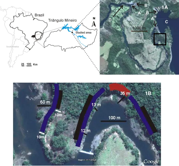
This study was conducted in a riparian forest (between 18°47´40”S, 48°08’57”W and 18°47´51”S, 48°08’43”W) located in the Amador Aguiar Dam influence area. For dam construction part of river was diverted by a 27m spillway reducing the flow over a 10km sector from December 2005. This river sector, where water flow was reduced, is called the “Reduced Outflow Stretch” (Trecho de Vazão Reduzida – ROS Figure 1.1). The spillway reduced the water flow from 359m3.s
-1 to 7m3.s-1. Thus, riparian forest near the riverbed in 2005 (Figure 1.2A) is now about 10–50 meters
further away from the direct water influence (Figure 1.2B). The average altitude is 595m with a low slope. The climate is Aw (Koppen 1948) with a dry winter (april to september) and a rainy summer (october to march), with an average annual temperature of 22°C and average rainfall of around 1595 mm (Santos & Assunção 2006).
Figure 1.1 - Study area image marked with a square showing studied area. A = Spillway and the beginning of Reduced Outflow Stretch, A’ = end of Reduced Outflow Stretch, B = hydroelectric dam, B’ = end of hydroelectric dam, C = artificial lake created by dam, D = river patch returns to normal flow.
Figure 1.2 - Satellite image of riparian forest on southern Brazil, object of this study, a = 2005 (T0) riparian plots figure and b = 2009 (T4) riparian forest showing flow reduction and the distance between forest with water after spillway construction. Plant sample were plotted along the black belt (a).
a
b
Soil - We carried out ten soil collections in riparian forest at three distinct depths: 0–10 cm, 20– 30cm and 40–50cm (total of 30 samples) along the ciliar forest. To verify the soil moisture variation we calculate soil moisture based on EMBRAPA methodology (EMBRAPA 1997). This separation is important because we try to substantiate how water flow reduction affects soil moisture at different depths. Then, we repeated soil sampling every three months to cover middle and end of rainy and dry seasons. We also repeated soil moisture collections over three distinct years: before the spillway construction (T0–2005), after (T1–2006) and during the third year of water flow reduction (T3– 2008).
We performed some soil moisture analyses for the three collections times, T0, T1 and T3. First to check the soil data normality we performed Lilliefors test, but soil data did not presented normality. Then we used non-parametric Wilcoxon test with all soil moisture results collected (near and far from shore together) over the years for the three soil depths. To compare effects of flow reduction on the seasons we performed a Kruskall-Wallis (a non parametric test for ANOVA) analysis followed by a post-hoc median test. All these analyses were performed in Systat 10.2 program (Wilkinson 2002).
Plant Sampling - The first inventory (T0) was carried out during the 2005 year after rain season on 110 plots of 10x10m in riparian forest, at 0-10 m and 10-20 m of distance to the river. All trees with a diameter at breast height (DBH) of 4.77cm were tagged with aluminum labels. The diameter of stem was measured at 1.30 m from the ground and in multiple stems all live tillers were also measured at 1.30m. The first inventory of results were published by Rodrigues et al. (2010). Second (T2) and third (T4) inventories were carried out in early 2008 and 2010, respectively two and four years after spillway construction (occurred in the december of 2005). These sampling methods followed the same procedure of first inventory. New individuals that met the inclusion criteria (recruits) were measured and identified. Mortality refers to standing dead trees, fallen trees or individuals which were not found. We prepared tree mortality distributions into classes of diameter using class intervals with exponentially increasing ranges of intervals of T0–T4. All the reproductive botanical material were inserted on Herbarium Uberlandense, and the species
nomenclature and synonymies follow Missouri Botanical Garden web site (http://www.tropicos.org/).
published together. Shannon-Weaver is the most popular index and is widely used in phytosociological and dynamic studies. Simpson is a good measure of diversity because it only varies between 0 (minimum diversity) and 1 (maximum diversity) which facilitates comparisons. To compare changes in diversity we performed statistical analyses between the three periods for each index. For Shannon we applied Hutcheson t test (Hutcheson 1970), and to Simpson index we followed the procedures suggested by Brower et al. (1998). We conducted a Wilcoxon test (a non-parametric test equivalent to Student t test) between T0-T2, T2-T4 and T0-T4 on the number of individuals and basal area using plots as samples. For evenness we performed the Pielou evenness indices (Brower et al. 1998).
Dynamics rates - We based community dynamics on mortality, recruitment, outgrowth and ingrowth rates. Annual mortality (m) and recruitment (r) were calculated in terms of annual exponensial rates (Sheil et al. 1995 and Sheil et al. 2000). Outgrowth annual rates (o) refers to basal areas of dead trees plus dead branch basal areas of living trees (decrement) and ingrowth annual rates (i) refers to basal areas of recruits plus growth in basal area of surviving trees (increment). Then we analyze mortality/recruitment rates and ingrowth/outgrowth annual rates of the most representative species (minimum of 10 individuals). Annual rates formulas used were,
m = 100 × {1-[(n0 - nm) /n0]1/t};
r = [1 - (1 - nr/nt)1/t ] × 100};
o = {1 - [(BA0 - BAm + BAd)/BA0]1/t} x 100 and
i = {1- [1 – (BAr + BAg)/BAt]1/t} x 100
where n0 is the original number of trees; nm is number of deaths; nr is number of recruits; nt is final
number of individuals; BA0 is original basal area; BAm is basal area of dead trees; BAd is basal area
of dead stems of living trees; BAr is basal area of recruits; BAg is growth basal area; BAt is final
To evaluate changes in forest we computed turnover rates for individuals and basal area through mortality-recruitment rates and outgrowth-ingrowth rates (Oliveira-Filho et al. 2007):
TN = (m + r) x 2-1;
TBA = (o + i) x 2-1
where TN is individuals turnover and TBA is basal area turnover. Then we evaluated net change (Korning & Balslev 1994) to individuals and basal area,
ChN = [(Nt/No)1/t - 1] x 100;
ChBA = [(BAt/BAo)1/t - 1] x 100
where ChN is individuals net change and ChBA is basal area net change and we develop an overall net change based on average of ChN and ChBA rates. All these analyses were conducted on each species with at least 10 individuals. Finally we evaluated the species individuals, basal area, and cover value (an average relative value between the number of individual and basal area) for species with at least 10 individuals, focusing on unstable species). However, due to large number of species, we only reported on those species that represented greatest changes in the community.
Results
Table 1.1. Wilcoxon test results (with “p “and “Z” values) for soil moisture in each season between different soil depths. MR = middle rainy season, ER = end rainy season, MD = middle dry season, ED = end dry season, T0 = before spillway construction, T1 = one year after and T3 = three years after flow reduction in a riparian forest in southern Brazil. In bold p < 0.05 and in italic p < 0.10.
0 – 10 cm 20 – 30 cm 40 – 50 cm
p\Z
values T0 T1 T3 T0 T1 T3 T0 T1 T3
T0 - 1.478 -0.866 - 0.663 -0.357 - 0.968 -0.153
MR T1 0.139 - -2.090 0.508 - -0.663 0.333 - -0.764
T3 0.386 0.037 - 0.721 0.508 - 0.878 0.445 -
T0 - 0.459 1.580 - -1.682 0.153 - -0.764 0.968
ER T1 0.646 - 1.988 0.093 - 2.293 0.445 - 1.784
T3 0.114 0.047 - 0.878 0.022 - 0.333 0.074 -
T0 - -2.803 -2.599 - -0.764 -1.682 - 0.153 -0.255
MD T1 0.005 - -0.051 0.445 - -2.497 0.878 - -0.357
T3 0.009 0.959 - 0.093 0.013 - 0.799 0.721 -
T0 - -2.599 -1.172 - -1.955 -1.580 - -2.073 -1.172
ED T1 0.009 - 1.682 0.050 - 0.969 0.038 - 1.244
T3 0.241 0.093 - 0.114 0.333 - 0.241 0.214 -
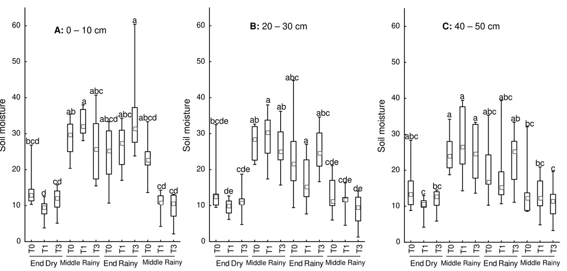
In general, there were no significant differences between years. In all years, middle and end of rainy season are obviously more moist (Figure 1.3) at all three depths. However, middle of dry season before dam construction was as humid as moister seasons of that year (Figure 1.3). Nevertheless, after dam construction and water flow reduction of middle dry season became as dry as the end of dry season. This effect was best demonstrated at 0-10cm depth (Figure 1.3 A), probably because this depth was more river dependent than deeper soil layers, which may be more subjected to moisture from groundwater. In other layers (20-30cm and 40-50cm) test was not significant; however, demonstrates a moisture reduction tendency after dam construction (Figure 1.3 B, C). These results (Table 1.1) show that the ground surface was more affected by reduction in water flow on river than deeper layers and became drier (Figure 1.3) after flow reduction which was mainly evident in middle of dry season.
Floristic changes - After four years of water flow reduction the richness in riparian forest varied little (92 in T0 and T2, and 93 in T4). Two species were found in T0 and T2 (Machaerium villosum
and Rudgea virburnoides) represented by a single tree, but these individuals were killed throughout
sericea, Eugenia involucrata and Lonchocarpuscultratus. As well as richness, diversity seems not
to have been affected even four years after flow reduction, neither in number of individuals either for basal area (Table 1.2). Also there was no change in evenness in number of individuals, although a reduction in basal area evenness after four years of damming is perceptible (Table 1.2).
Table 1.2 - Diversity indexes (with respective tests results) and evenness for number of individuals and basal area in a riparian forest in southern Brazil. Different letters indicate significant variation between times.
Number of individuals Basal area
T0 T2 T4 T0 T2 T4
Absolute values 1405 1369 1288 45.60 44.75 44.21 Shannon Index (H’) 3.659a 3.714a 3.685a 3.253a 3.273a 3.144a Simpson Index (1-D) 0.955a 0.959a 0.960a 0.955a 0.953a 0.939a Pielou Evenness 0.807 0.819 0.809 0.717 0.722 0.690
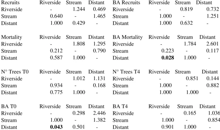
Structure changes - There was a reduction in number of individuals and basal area between the years evaluated (Table 1.3). For number of individuals there was a clear reduction four years after water spillway construction (4.05%) and marginally statically significant difference after first two years (2.56%, Table 1.3). However, to basal area only the periods T0-T2 (loss of 1.86%) and T0-T4 (loss of 3.04%, Table 1.3) presented differences that was marginally statistically significant. These decreases are mainly due to high mortality (268 trees) and lower recruitment (151) along four measurement years (Table 1.4). Despite of the high increment (7.68m2 in four years), high mortality added to strong loss of stems provided a greater loss in basal area than gain (Table 1.4). Analysis of mortality by diameter classes demonstrates a higher mortality in two first classes (4.77cm until 9.9cm and 10cm until 19.9cm), with 131 and 95 dead trees respectively. The third class (20cm until 39.9cm) and fourth class (higher than 40cm of diameter) only presented 29 and 14 respectively. These results demonstrated that smaller trees (smaller than 20cm of diameter) were most negatively affected by disturbance, representing 84% of dead trees in this riparian forest.
Table 1.3 - Wilcoxon test between basal areas in the plots in T0, T2, T4 in a riparian forest in southern Brazil. In bold p < 0.05 and in italic p < 0.10
Number of individuals (p\Z) Basal área (p\Z)
Years T0 T2 T4 T0 T2 T4
T0 - -3.655 -3.500 - 1.048 1.601
T2 0.096 - -1.664 0.092 - 1.873
Table 1.4 - Dynamics parameters in four years of water flow reduction in a riparian forest in southern Brazil. N = number of individuals, BA = basal area)
Parameters T0-T2 T2-T4 T0-T4
Mortality (N) 125 143 268
Recruitment (N) 89 62 151
Mortality (m2) 2.80 3.26 6.07 Recruitment (m2) 0.22 0.17 0.39
Decrement (m2) 1.82 1.57 3.39
Increment (m2) 3.55 4.13 7.68
T 1 T 3 T 0 T
1 T3
T
0
End Dry Half Rainy End Rainy Half Dry
T
1
T
3 T0
T 1 T 3 T 0 0 10 20 30 40 50 60 S o il m o is tu re a a abc
a abc abc
bc
c bc
bc c
Middle Rainy Middle Rainy 0 10 20 30 40 50 60 S o il m o is tu re T 1 T 3 T 0 T
1 T3
T
0
End Dry Half Rainy End Rainy Half Dry
T
1
T
3 T0
T 1 T 3 T 0
Middle Rainy Middle Rainy
a ab ab a abc bcde abc cde cde cde de de ab
Figure 1.3. Box-Plot representation to Kruskall-Wallis test to distinct depths before spillway construction (T0), one year after (T1) and three years after flow reduction (T3) in a riparian forest in southern Brazil. Dashes = range, Bars = interval between first and third quartile, square = median. Results detail on Appendix 1.
A: 0 – 10 cm B: 20 – 30 cm C: 40 – 50 cm
T 1 T 3 T 0 T
1 T3
T
0
End Dry Half Rainy End Rainy Half Dry
T
1
T
3 T0
T 1 T 3 T 0 0 10 20 30 40 50 60 S o il m o is tu re a ab abcd abcd abc
a
cd
abc
bcd
cd
d cd
Dynamic rates - Tree dynamics presented higher mortality rates than recruitment (Table 1.4). The same occurred between outgrowth and ingrowth annual rates, especially due low recruits basal areas and due high mortality and basal area loss by trees with dead stems. All these rates reveal a faster tree dynamic community than other riparian and tropical forests, represented by high turnover rates of number of individuals and basal area (Table 1.4). At the same time with a strong negative balance exemplified by a negative net rate on number of individuals and basal area.
While some species showed slow dynamics with low mortality and recruitment rates (lower rates than the entire community – Table 1.4, Figure 1.4A), others have high rates with high recruitment and/or mortality (Figure 1.4A). From those species with fast dynamics, only three species had a positive individual’s net change, meanwhile another 14 had a negative individual’s net change. Thus, the flow reduction in general affects more species negatively than positively.
The same is seen to ingrowth/outgrowt rates (Figure 4B) because eight species had rates lower than the entire community. Nine species presented ingrowth larger than outgrowth and had a positive basal area net change. However, a further 16 have more outgrowth rates higher than ingrowth, and possessed a negative basal area net change. Hence, negative impacts of water flow reduction were intense for basal area and individuals in this riparian forest and surpassed any positive effects.
Figure 1.4 - Comparison of mortality/recruitment rates (A) and outgrowth/ingrowth rates (B) in species with 10 or more individuals in a riparian forest in southern Brazil. Square = community net change, triangles = species with positive individuals net changes, circles = species with negative individuals net changes, blue diamond = species with individual net changes lower than community and black diamond = species with individuals net changes lower than community but with area basal net change higher than community. Species Legend in Table 5.
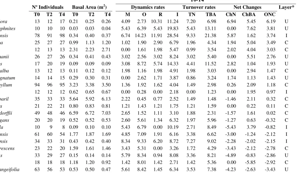
Species with high individuals turnover (higher than 3.5 of TN, Table 1.5) are most typically from understory or forest edge (Siparuna guianensis, Myrcia laruotteana, Byrsonima laxiflora,
Xylopia aromatica, Bauhinia ungulata, Coccoloba mollis, Cousarea hydrangeaefolia,
Erythroxylum daphnites, Matayba guianensis, Cordieria sessilis, Alibertia edulis and Casearia
sylvestris), except Inga vera, I. laurina and Hirtella gracilipes; three sub-canopy/canopy species
which are related to moist environments (riparian and gallery forests). Otherwise, those species with low rates (lower than 3.0 of TN, Table 1.5) are mostly from canopy (Apuleia leiocarpa, Terminalia
glabrescens, Tabebuia roseo-alba, Ficus sp1, Protium heptaphyllum, Copaifera langsdorffii,
Hymenaea courbaril, Platypodium elegans, Pouteria torta, Andira anthelmia, Salacia elliptica,
Acacia polyphylla) excepting Cheiloclinium cognatum, a typical understory species.
Most of the high turnover species (11 of 15) had a negative balance between mortality/recruitment and outgrowth/ingrowth, except S. guianensis, B. laxiflora, E. daphnites and
C. sessilis (Table 1.5). However, some low turnover (7 of 13) species have a zero/positive balance
between mortality/recruitment and/or outgrowth/ingrowth. From these low turnover species analyzed, four have both negative balances (Tapirira guianensis, Ormosia arborea, Zanthoxyllum
riedelianum and Myrcia splendens) and one a zero/positive balance (Unonopsis lindimanii). Thus,
most of the species (19, Table1.5) have a negative overall net rate (ONR) and seven show an ONR lower than five negative. Then, from 14 species with positive ONR (Table 1.5) only B. laxiflora
exceeded five.
All these results indicated that few species (mostly from canopy) were subjected to only minor changes, and can be considered stable in this riparian forest even after flow reduction. Most species, however, had experienced a high death rate and/or loss of basal area, demonstrated the negative effects of lack of moisture. Moreover, the most severe negative effects of moisture reduction occurred to understory species and those associated with water resources. Figure 1.5 represents the species with major contributions to community changes. H. gracilipes, I. vera, A.
edulis (water associated sub-canopy understory species), I. laurina (canopy water associated
species), C. hydrangeaefolia, C. mollis and P. torta (understory-subcanopy species) were the more
negatively affected species which strongly influences the community density and/or basal area reduction.
Only two species experienced major positive changes in this riparian forest: S. guianensis,
within an increase in number of individuals and A. leiocarpa with an increase in basal area – Figure
water associated, were the most negatively affected with strong mortality and basal area loss (H.
gracilipes, I. vera, A. edulis). With the high reduction in individuals and basal area of some species
below canopy and a population increase (S. guianensis) in a short time period (four years), it is
Table 1.5 - Species dynamic rates between T0 – T4 in descending order of Overall net change (ChN+ChAB)/2) to species with 10 or more individuals. M = mortality rate, O = outgrowth rate, R = recruitment rate, I = ingrowth rate, TN = individuals turnover, TBA = basal area turnover, ChN = individuals net chance, ChBA = basal area net change, ONC = overall net change; U = understory, I = intermediary, C = canopy (*Rodrigues et al 2010 classification) in a riparian forest in southern Brazil.
T0-T4
Nº Individuals Basal Area (m2) Dynamics rates Turnover rates Net Changes Layer*
Codes Species T0 T2 T4 T0 T2 T4 M O R I TN TBA ChN ChBA ONC
b Byrsonima laxiflora 13 12 17 0.21 0.25 0.26 4.09 2.73 10.31 11.24 7.20 6.98 6.94 5.45 6.19 U
e Erythroxylum daphnites 10 10 10 0.03 0.03 0.04 5.43 6.39 5.43 19.83 5.43 13.11 0.00 7.62 3.81 U
a Siparuna guianensis 78 91 98 0.34 0.40 0.37 6.74 14.23 11.91 28.54 9.33 21.38 5.87 1.62 3.74 I
x Apuleia leiocarpa 25 27 27 0.99 1.13 1.20 1.02 1.90 2.90 6.79 1.96 4.34 1.94 5.04 3.49 C
y Ficus sp1 12 13 13 2.31 2.23 2.71 0.00 1.61 1.98 5.47 0.99 3.54 2.02 4.04 3.03 C
w Unonopsis lindmanii 26 27 26 0.34 0.41 0.43 3.02 2.56 3.02 8.24 3.02 5.40 0.00 5.51 2.76 U
f Cordieria sessilis 17 20 19 0.09 0.09 0.09 3.08 8.72 5.74 14.33 4.41 11.52 2.82 1.04 1.93 U
z Tabebuia roseo-alba 13 12 13 0.11 0.12 0.12 1.98 1.16 1.98 4.91 1.98 3.03 0.00 2.94 1.47 C
- Cheiloclinum cognatum 14 14 15 0.29 0.30 0.31 0.00 2.62 1.71 3.87 0.86 3.24 1.74 1.13 1.43 U
- Protium heptaphyllum 94 96 95 3.23 3.38 3.50 1.36 1.92 1.62 4.04 1.49 2.98 0.26 2.09 1.18 C
- Salacia elliptica 12 12 12 0.62 0.65 0.67 0.00 0.28 0.00 2.18 0.00 1.23 0.00 1.95 0.97 I
- Hymenaea courbaril 35 33 33 5.64 5.92 6.13 2.22 0.45 0.77 2.52 1.49 1.48 -1.46 2.11 0.32 C
- Andira anthelmia 21 22 21 0.80 0.83 0.81 1.21 1.43 1.21 1.75 1.21 1.59 0.00 0.22 0.11 C
- Copaifera langsdorffii 49 48 46 6.59 6.72 7.03 2.65 1.52 1.11 3.10 1.88 2.31 -1.57 1.61 0.02 C
v Platypodium elegans 20 20 19 0.52 0.52 0.53 2.60 5.61 1.34 6.32 1.97 5.96 -1.27 0.63 -0.32 C
q Acacia polyphylla 10 9 8 0.09 0.10 0.10 5.43 6.79 0.00 10.19 2.71 8.49 -5.43 3.79 -0.82 I
u Tapirira guianensis 61 60 54 1.77 1.87 1.69 4.85 7.09 1.91 6.16 3.38 6.62 -3.00 -1.24 -2.12 I
d Matayba guianensis 34 33 31 0.43 0.42 0.40 8.34 9.33 6.20 8.72 7.27 9.02 -2.28 -2.02 -2.15 I
- Terminalia glabrescens 23 22 20 1.59 1.61 1.46 3.43 5.31 0.00 3.26 1.72 4.29 -3.43 -2.12 -2.78 C
k Myrcia splendens 33 29 27 0.15 0.14 0.14 5.79 8.34 0.94 8.08 3.36 8.21 -4.89 -0.83 -2.86 U
t Pouteria torta 18 18 18 1.18 1.20 0.92 1.42 8.01 1.42 2.71 1.42 5.36 0.00 -5.85 -2.92 C
r Zanthoxyllum riedelianum 12 10 9 0.30 0.31 0.30 6.94 4.80 0.00 4.33 3.47 4.56 -6.94 -0.50 -3.72 C
n Hirtella gracilipes 174 171 151 4.41 3.78 3.68 5.63 10.20 2.23 6.30 3.93 8.25 -3.48 -4.45 -3.97 I
c Casearia sylvestris 25 22 20 0.18 0.16 0.15 7.88 8.65 2.60 6.37 5.24 7.51 -5.43 -3.26 -4.34 U
s Ormosia arborea 17 17 16 0.45 0.49 0.33 3.08 13.66 1.60 7.09 2.34 10.37 -1.50 -7.26 -4.38 C
g Bauhinia ungulata 40 40 27 0.23 0.27 0.21 12.92 14.44 3.93 14.60 8.42 14.52 -9.36 -1.74 -5.55 U
l Inga laurina 70 61 59 4.49 3.57 3.13 5.85 17.49 1.74 9.77 3.80 13.63 -4.18 -8.68 -6.43 C
o Alibertia edulis 74 68 62 0.70 0.53 0.49 6.73 13.49 2.51 6.16 4.62 9.83 -4.33 -8.81 -6.57 U
c Xylopia aromatica 20 19 17 0.37 0.27 0.24 13.88 14.94 10.31 6.97 12.10 10.96 -3.98 -10.29 -7.14 I
j Coccoloba mollis 59 52 43 0.61 0.52 0.38 9.26 19.41 1.79 10.11 5.53 14.76 -7.60 -11.05 -9.33 I
i Inga vera 38 29 23 1.00 0.86 0.63 12.77 14.03 1.11 3.60 6.94 8.81 -11.80 -10.90 -11.35 I