Ground motion simulation for dynamic structural
analysis: pros and cons
J.M.C. Estêvão
University of Algarve, ISE, Portugal C.S. Oliveira
Instituto Superior Técnico, Lisbon, Portugal
SUMMARY:
In many seismic codes the use of simulated ground motions for dynamic structural analysis is already considered. However, from the structural engineer point of view, the use of such simulated accelerograms is not very attractive, mainly because more seismological knowledge background is needed. For this reason, a user friendly freeware computer program named SIMULSIS was developed to help structural engineers to generate simulated accelerograms. A new finite-fault stochastic method was developed for ground motion simulation and implemented in the program together with an equivalent linear model that accounts for superficial soil dynamic amplification. The capabilities of the program and the precision of results produced are illustrated by the simulations carried out for two recorded earthquakes. Moreover, some suggestions related to the use of the developed computer program not only for seismic structural analysis purposes but also in the future generation of hazard maps are presented.
Keywords: Simulated accelerograms; Stochastic methods
1. INTRODUCTION
According to many seismic codes namely the Eurocode 8 (CEN, 2004), time-history representation of seismic action can be divided in three major groups: recorded accelerograms, artificial accelerograms (synthetic accelerograms generated so as to match an elastic response spectra), and simulated accelerograms (synthetic accelerograms generated through a physical simulation of source and travel path mechanisms).
In many regions like Portugal where the historical knowledge of massive destruction due to the 1755 earthquake exists, but not enough strong-motion records for engineering purposes are available, the alternative is to use “synthetic” accelerograms. For a structural engineer the use of artificial accelerograms is very attractive, mainly because they do not depend on seismological knowledge. However, it is now widely accepted that the use of artificial accelerograms in seismic nonlinear analysis have many problems, because they tend to be particularly unrealistic (Bommer and Acevedo, 2004). This is the reason why simulated accelerograms can be a valid option.
There are many methods available for strong ground motions simulations, being the stochastic methods an “Engineering” approach to the problem with successful comparisons of predicted and recorded data (Erdik and Durukal, 2006). Recently, many computer programs for stochastic earthquake ground motion simulation have been developed for seismic hazard analysis purposes. Boore’s point source method was implemented in SMSIM computer program (Boore, 1983, Boore, 2003, Boore, 2005). FINSIM (Beresnev and Atkinson, 1998) and EXSIM (Motazedian and Atkinson, 2005) are other well known programs for stochastic ground motion simulation, which adopt a finite fault model. Another finite fault model, including site effects, was developed (Carvalho et al., 2008) and used for Portugal seismic risk assessment (Oliveira, 2006).
purposes. SIMULSIS freeware software was created to be user friendly, with a graphical input and output interface.
2. PROGRAM SIMULSIS
SIMULSIS is a program developed in Object Pascal. The first version of the program had some difficulties in simulating earthquakes (Estêvão and Oliveira, 2008). Later, some changes were introduced and lead to several improvements (Estêvão and Oliveira, 2010). Finally, more modifications were included in the present version (ver. 1.02), which seems to be much more reliable (Estêvão, 2012). The user has many simulation options and he is allowed to select the most suitable method according to his objectives.
2.1. Simulation developed methods
The simulated accelerogram results from the contribution of a number of small earthquakes as subfaults that comprise a big fault. A large fault is divided in NF subfaults and each subfault is considered as a point source event. In SIMULSIS the rupture spreads radially from the hypocenter, with a constant or a variable rupture velocity Vri (depending on the preference of the user) on each subfault i, so time series results from a superposition of sinusoidal waves that are summed with a proper delay
(
)
∑ ∑
= = ∆ ω θ + ∆ ⋅ ω ⋅ = NF i i 1 i N 1 n i , n i n ) t ( n , i ) t ( g A cos t a (2.1)The wave amplitude Ai,n(∆ti) is the contribution of the point source i to the frequency ωn (equal spaced at ∆ωi), with random phase angles θn,i
(
n 0i) (
n i)
R( ) ( )
n S n i F i i ) t ( n , i F ,M P ,R H H T 2 ) t ( g A ⋅ ω ⋅ ω ⋅ ω ⋅ ω ⋅ π ω ∆ ⋅ ⋅ = (2.2)TF is the total equivalent point source fault rupture duration, and Fi(ωn,M0i) is the point source spectrum of shear waves, of each subfault (Estêvão, 2012). P(ωn,Ri) is a path attenuation function, and HR(ωn) is a filter (function of a
cut-off frequency
ω
max=2·π·f
maxand of a reduction parameter k
0) that accounts for the diminution of the high-frequency motions in a rock outcropping reference site (Boore, 1983, Boore, 2003). HS(ωn) is a nonlinear soil transfer function for S waves, obtained from an equivalent linear analysis of a one-dimensional “soil column” with a procedure similar to the implemented in SHAKE91 program (Idriss and Sun, 1992), but with the maximum soil distortion computed in frequency domain using stochastic methods (Carvalho et al., 2008).The parameters of the deterministic envelope function gi(t) are obtained so that an effective duration (Bommer and Martinez-Pereira, 1999) between two values of Arias intensity is accomplished for each point source (Estêvão, 2012).
Two methods were implemented in SIMULSIS. The first method developed (A) was based on several concepts that support the program EXSIM (Motazedian and Atkinson, 2005) but with some modifications (Estêvão, 2012). The concepts of dynamic corner frequency (Motazedian and Atkinson, 2005) and active pushing area (Motazedian and Moinfar, 2006) were also adopted.
In order to improve simulation results of past earthquakes, mainly in time domain, another method (B) was developed and implemented in SIMULSIS. The main difference between methods A and B is related to the determination of corner frequency (Estêvão, 2012).
Based on our experience, we recommend method A for structural analysis purposes when constant slip distribution and rupture velocity are adopted for the ground motion simulations. The method B seems to be more suitable to reproduce recorded accelerograms when non constant slip distribution and rupture velocity are adopted.
2.2. Program validation
To demonstrate the capabilities of the programme, SIMULSIS was used to simulate two past earthquakes.
2.2.1. Simulation of the 28 September 2004 Parkfield earthquake
The 2004 Parkfield earthquake was a predicted seismic event that occurred in the California. For that reason there is much information about it. The simulations were carried out for two different sites at Turkey Flat (near each other), where the earthquake was recorded (Table 2.1). Before the earthquake occurrence, this place was selected for a soil amplification blind test (Tucker and Real, 1986, Real, 1988, Real et al., 2006). For this reason the source of this earthquake is well known and site parameters are perfectly characterized, so we believe that it is a good place to validate program SIMULSIS.
Simulations were carried out for sites #3 and #4 of Turkey Flat (Fig. 2.1) considering the fault rupture and slip distribution proposed by Chen Ji (Ji, 2004), with a variable rupture velocity with a mean value of 2.8 km/s (Liu et al., 2006), and a stress drop of 150 bar, which is in the range of values obtained for the rupture (Allmann and Shearer, 2007). Method B of SIMULSIS was adopted (Estêvão, 2012).
Table 2.1. Parkfield - Turkey Flat stations information (CESMD - Center for Engineering Strong Motion Data)
CGS - CSMIP Station Latitude Longitude Site Geology Turkey Flat #3 Station No. 36519 35.8868 N 120.351 W Shallow alluvium Turkey Flat #4 Station No. 36518 35.8915 N 120.353 W Soft rock (sandstone)
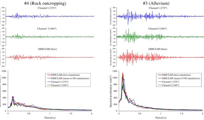
First, the parameter fmax was established to 10 Hz (k0 = 0), to adjust peek acceleration at site #4 (rock outcropping). Than, soil profile (Tucker and Real, 1986, Real, 1988) of site #3 (alluvium) was introduced in SIMULSIS. Simulation results are presented in Fig. 2.2 (Estêvão, 2012), and seem to show a good approximation to the recorded values, reproducing the observed soil amplification.
#4 (Rock outcropping) #3 (Alluvium) -260 -156 -52 52 156 260 A cc e le ra ti o n ( c m /s 2) Channel 1 (270°) -260 -156 -52 52 156 260 A c ce le ra ti o n ( c m /s 2) Channel 3 (360°) -260 -156 -52 52 156 260 A c c el e ra ti o n (c m /s 2) SIMULSIS (best) -260 -156 -52 52 156 260 A cc e le ra ti o n ( c m /s 2) Channel 1 (270°) -260 -156 -52 52 156 260 A cc e le ra ti o n ( cm /s 2) Channel 3 (360°) -260 -156 -52 52 156 260 A c c el e ra ti o n (c m /s 2) SIMULSIS (best) 0 200 400 600 800 1000 1200 0 0.5 1 1.5 2 S p ec tr al a cc el er at io n ( cm /s 2) Period (s)
SIMULSIS (best simulation) SIMULSIS (mean of 100 simulations) Channel 1 (270°) Channel 3 (360°) 0 200 400 600 800 1000 1200 0 0.5 1 1.5 2 S p ec tr al a cc el er at io n ( cm /s 2) Period (s)
SIMULSIS (best simulation) SIMULSIS (mean of 100 simulations) Channel 1 (270°)
Channel 3 (360°)
Figure 2.2. Recorded and simulated accelerograms (cm/s2) and corresponding response spectra at Turkey Flat.
2.2.2. Simulation of the 27 March 2010 Maule earthquake
This Chile subduction earthquake (Mw=8.8) produced important soil amplification effects, which were evident in the acceleration response spectra of many records obtained in different locations (Saragoni et al., 2010, Boroscheck et al., 2010). Moreover, the simulation of this earthquake is more challenging for SIMULSIS, because we do not have the exact knowledge about the soil layers characteristics of each station. For this reason, this earthquake is also a good test for the capability of SIMULSIS to simulate the earthquake effects on a site where the real soil conditions are unknown.
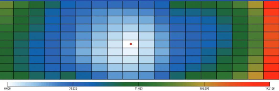
These new simulations were carried out considering the rupture solution proposed by Gavin Hayes (Hayes, 2010). The slip distribution and rake is presented at Fig. 2.3. Rupture location is presented at Fig. 2.4.
Figure 2.3. 2010 Chile earthquake slip distribution and rake adopted for the simulations.
Simulations were carried out using method B of SIMULSIS, for a central site of Santiago, and compared with the recorded ground motions (Boroscheck et al., 2010). We adopted a stress drop of 100 bar, with ρ=2.8 g/cm3 and β=3.7 km/s, which are the density and shear-wave velocity in the vicinity of the source, respectively. The path attenuation expressions adopted are the same that were
adopted in North American studies (Atkinson and Boore, 1995). It was considered a variable rupture velocity, with a mean value of 2.25 km/s. The time rupture adopted is presented at Fig. 2.5. Site ground motion durations were calculated using empirical expressions (Reinoso and Ordaz, 2001).
Figure 2.4. 2010 Chile earthquake rupture location adopted for the simulations.
Figure 2.5. 2010 Chile earthquake source subfault time rupture adopted for simulations.
As already mentioned, we do not know the exact site soil profile characteristics. In contrast with 2004 Parkfield earthquake simulation sites (where there exists a good soil characterization), the site parameters adopted for 2012 Chile earthquake are only an approximation which leads to an acceptable simulation results. The adopted characteristics were based in several studies existent for the city of Santiago de Chile (Pilz et al., 2011, Bonnefoy-Claudet et al., 2009). A soil column with 150 m, with three layers with different parabolic variation of shear wave velocity (VS), was considered (fmax = 6 Hz). The VS of superficial layer (20 m) is between 120 and 350 m/s, the VS of second layer (30 m) is between 450 and 700 m/s, and VS of the third layer (100 m) is between 800 and 1700 m/s. Bedrock VS was established to 3800 m/s. All these values were selected through a trial and error process. It is possible that different parameters (more close to the reality) could lead to better simulation results. SIMULSIS simulation results are presented at Fig. 2.6.
-400 -300 -200 -100 0 100 200 300 400 A c ce le ra ti o n (c m /s 2) Channel 1 -400 -300 -200 -100 0 100 200 300 400 A c ce le ra ti o n (c m /s 2) Channel 2 -400 -300 -200 -100 0 100 200 300 400 A cc e le ra ti o n ( c m /s 2) SIMULSIS (best) 0 200 400 600 800 1000 1200 0 0.5 1 1.5 2 S p ec tr al a cc el er at io n ( cm /s 2) Period (s)
SIMULSIS (best simulation) SIMULSIS (mean of 20 simulations) Channel 1
Channel 2
Figure 2.6. Recorded and simulated accelerograms (cm/s2) and corresponding response spectra at Santiago.
3. DISCUSSION
A detailed sensitivity analysis of several factors was carried out using SIMULSIS results (Estêvão, 2012). The study considers the influence of earthquake focus location relatively to the fault plane, fault plane discretisation, rupture velocity, asperity locations, subfault rupture duration, stress drop (Fig. 3.1A) and geological site effects factors, such as fmax value (Fig. 3.1B), soil surface VS,30 value, impedance contrast and plasticity index variation. The study also included a point versus fault rupture results comparison. We believe that this sensitivity analysis was very important to improve earthquake simulation results. The knowledge that this study allowed do obtain was very useful to carry out all the simulations presented in this work.
(A) (B) 0 100 200 300 400 500 0 0.5 1 1.5 2 S p ec tr al a cc el er at io n ( cm /s 2) Period (s) 50 bar 100 bar 150 bar 0 100 200 300 400 500 0 0.5 1 1.5 2 S p ec tr al a cc el er at io n ( cm /s 2) Period (s) 5 Hz 10 Hz 15 Hz
Figure 3.1. Example of the influence of (A) stress drop and (B) fmax on the response spectra simulation results.
The SIMULSIS results of 2004 Parkfield earthquake simulation seems to be very close to the recorded values, for both sites (#3 and #4). Peak accelerations are almost exact and simulated response spectra match the recorded values at low and high period values. Probably, these good results are due to the accurate knowledge about source rupture and site characteristics (namely layers definition, shear wave velocity, density and plasticity index), and demonstrate SIMULSIS capabilities of reproducing ground motions characteristics.
than one second. One explanation for this problem could be the adopted source rupture solution, because the simulations exhibits greater durations when compared with recorded accelerograms. Probably the use of just one attenuation law is not suitable for such great rupture dimensions. Another explanation for the observed differences can be related to site soil profile, which is not well defined. In future, further simulations should be carried out with different source rupture solution and site characteristics, to improve 2010 Chile earthquake results.
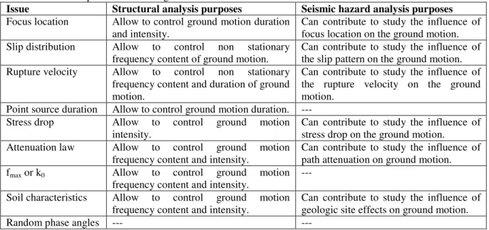
Simulations that we carried out with SIMULSIS have revealed pros and cons of using simulated stochastic ground motion accelerograms for structural analysis purposes, and also for seismic hazard analysis purposes. Some of those pros and cons, which we consider most important, are presented in Tables 3.1 and 3.2.
Table 3.1. Selected pros of simulated ground motions
Issue Structural analysis purposes Seismic hazard analysis purposes
Focus location Allow to control ground motion duration and intensity.
Can contribute to study the influence of focus location on the ground motion. Slip distribution Allow to control non stationary
frequency content of ground motion.
Can contribute to study the influence of the slip pattern on the ground motion. Rupture velocity Allow to control non stationary
frequency content and duration of ground motion.
Can contribute to study the influence of the rupture velocity on the ground motion.
Point source duration Allow to control ground motion duration. --- Stress drop Allow to control ground motion
intensity.
Can contribute to study the influence of stress drop on the ground motion.
Attenuation law Allow to control ground motion frequency content and intensity.
Can contribute to study the influence of path attenuation on ground motion. fmax or k0 Allow to control ground motion
frequency content and intensity.
--- Soil characteristics Allow to control ground motion
frequency content and intensity.
Can contribute to study the influence of geologic site effects on ground motion.
Random phase angles --- ---
Table 3.2. Selected cons of simulated ground motions
Issue Structural analysis purposes Seismic hazard analysis purposes
Focus location --- It is impossible to predict, so it is advisable to use the worst and best case scenarios.
Slip distribution --- The same problem as for focus location. Rupture velocity --- The same problem as for focus location. Point source duration --- The same problem as for focus location. Stress drop --- The same problem as for focus location. Attenuation law --- Should be selected from previous
recorded earthquakes.
fmax or k0 --- It has a great influence on the results. It
seems advisable to use local site values obtained from previously recorded earthquakes or from ambient noise measurements.
Soil characteristics --- It has a great influence on the results. Must have a detailed soil layers characterization.
Random phase angles Each simulation gives a different result, so it is advisable to use a result as near as possible of mean value.
Each simulation gives a different result, so it is advisable to use the mean value.
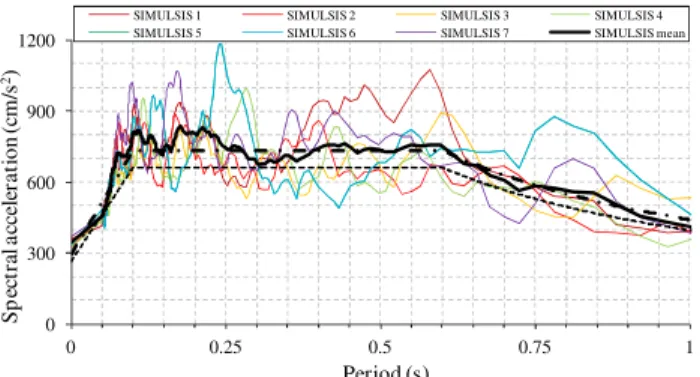
It seems that stochastic ground motion simulations have more pros than cons, because normally simulation results must be close to a known target response spectrum. For example, EC8 indicates that a minimum of three simulated accelerograms should be generated so as to match an elastic response
spectrum, within some limits (Fig. 3.2). 0 300 600 900 1200 0 0.25 0.5 0.75 1 S p ec tr al a cc el er a ti o n ( cm /s 2) Period (s)
SIMULSIS 1 SIMULSIS 2 SIMULSIS 3 SIMULSIS 4 SIMULSIS 5 SIMULSIS 6 SIMULSIS 7 SIMULSIS mean
Figure 3.2. Example of using simulated accelerograms according to EC8 (Estêvão and Oliveira, 2010).
We believe that for structural analysis purposes the bigger disadvantage is related to random phase angles generation scheme, because results are different for each simulation carried out with the same simulation parameters. However, this problem can be minimized using only the simulation results that are closer to the mean values. Future work on phase angle spectrum evaluation would be helpful to minimize this problem.
For seismic hazard analysis, stochastic ground motion simulations have more problems, because the results are very dependent on source, path and site parameters. For a given earthquake magnitude, there are many possible patterns for slip distribution, rupture velocities and stress drop, for example. Only if the future earthquake presents, exactly, all the characteristics adopted for the simulations, the results could match the future records. It is obvious that this hypothesis has a low probability to occur, so it is nearly impossible to predict the seismic effects using programs like SIMULSIS. However, they can be very useful tools to evaluate future possible earthquake scenarios.
It is important to find a reliable way of using stochastic ground motion simulations in seismic risk assessment, in together with more traditional approaches.
All the simulations carried out with SIMULSIS have shown a great influence of geological site characteristics on results. This can explain some damage concentrations in several earthquake affected areas.
4. CONCLUSIONS
Earthquake simulations presented in this work, namely the 2004 Parkfield earthquake simulations, allows us to conclude that SIMULSIS is able to reproduce ground motion effects, if a proper source, path and site parameters are considered.
For structural analysis purposes we did not find any important cons of using stochastic simulated ground motions to mach a target response spectrum. Probably is a better choice than using artificial accelerograms which seems to be less realistic. The major problem that we experienced was related to the random phase angles variation, which can be partially solved by selecting the accelerograms which are closer to the mean result values.
Whenever there is not a target response spectrum to match, the use of stochastic simulated ground motions for seismic hazard analysis purposes present pros and cons. Most of the cons are due to the uncertainty related with the rupture process, path and site characteristics. On other hand, pros are mostly related to the possibility of changing one variable and seeing what happens to ground motions, being like a virtual earthquake laboratory.
The use of stochastic simulated ground motions can be very useful to establish possible earthquake scenarios, for seismic hazard analysis purposes of regions where there are few earthquake strong motion records available. However, in face of our sensitivity analysis results, we believe that it should be done carefully, because of the influence of parameter variability on simulated earthquake results. The huge variability of stochastic simulation results, which depends on the earthquake and site characteristics, seems to indicate that it is impossible to predict the exact effect of a future earthquake using computer programs like SIMULSIS. The results of this kind of program should be understood as a mean possible earthquake scenario. However, if the statistical distributions of all parameters that influence earthquake results are considered, stochastic ground motion simulations can be very helpful for seismic hazard analysis purposes.
REFERENCES
Allmann, B. P. and Shearer, P. M. (2007). Spatial and temporal stress drop variations in small earthquakes near Parkfield, California. Journal of Geophysical Research. 112:B4, B04305.
Atkinson, G. M. and Boore, D. M. (1995). Ground-Motion Relations for Eastern North America. Bulletin of the
Seismological Society of America. 85:1, 17-30.
Beresnev, I. A. and Atkinson, G. M. (1998). FINSIM — a FORTRAN program for simulating stochastic acceleration time histories from finite faults. Seismological Research Letters. 69, 27-32.
Bommer, J. J. and Acevedo, A. B. (2004). The use of real earthquake accelerograms as input to dynamic analysis. Journal of Earthquake Engineering. 8:Special Issue 1, 43-92.
Bommer, J. J. and Martinez-Pereira, A. (1999). The effective duration of earthquake strong motion. Journal of
earthquake engineering. 3:2, 127-172.
Bonnefoy-Claudet, S., Baize, S., Bonilla, L. F., Berge-Thierry, C., Pasten, C., Campos, J., Volant, P. and Verdugo, R. (2009). Site effect evaluation in the basin of Santiago de Chile using ambient noise measurements. Geophysical Journal International. 176:3, 925-937.
Boore, D. M. (1983). Stochastic simulation of high-frequency ground motions based on seismological models of the radiated spectra. Bulletin of the Seismological Society of America. 73:6, 1865-1894.
Boore, D. M. (2003). Simulation of Ground Motion Using the Stochastic Method. Pure and Applied Geophysics.
160, 635-676.
Boore, D. M. (2005). SMSIM — Fortran programs for simulating ground motions from earthquakes:Version 2.3
- A Revision of OFR 96–80–A, Open-File Report of 00-509, U.S. Geological Survey, Menlo Park.
Boroscheck, R., Soto, P. and León, R. (2010). Maule Region Earthquake February 27, 2010 Mw=8.8, RENADIC Report 10/08, University of Chile, Santiago.
Carvalho, A., Zonno, G., Franceschina, G., Serra, J. B. and Costa, A. C. (2008). Earthquake shaking scenarios for the metropolitan area of Lisbon. Soil Dynamics and Earthquake Engineering. 28:5, 347-364. CEN (2004). Eurocode 8, Design of Structures for Earthquake Resistance-Part 1: general rules, seismic actions
and rules for buildings. EN 1998-1:2004, Comité Européen de Normalisation.
Erdik, M. and Durukal, E. (2006). Strong ground motions. In: ANSAL, A. (ed.) Recent advances in Earthquake
Geotechnical Engineering and Microzonation. Springer, Dorrecht, 67-100.
Estêvão, J. M. C. (2012). Seismic effects on the behavior of reinforced concrete buildings with infill walls. PhD thesis, Instituto Superior Técnico, UTL (in Portuguese).
Estêvão, J. M. C. and Oliveira, C. S. (2008). Stochastic ground motion simulation with geological site effects in damage assessment International Seminar on Seismic Risk and Rehabilitation of Stone Masonry
Housing, Horta, Faial. 61-64, CD015, 14 pag.
Estêvão, J. M. C. and Oliveira, C. S. (2010). Utilização de acelerogramas simulados na análise sísmica de estruturas. 8º Encontro Nacional sobre Sismologia e Engenharia Sísmica, Aveiro. 1-13, CD083 (in Portuguese).
Hayes, G. (2010). Updated Result of the Feb 27, 2010 Mw 8.8 Maule, Chile Earthquake, USGS.
http://earthquake.usgs.gov/earthquakes/eqinthenews/2010/us2010tfan/finite_fault.php (last accessed
April 2012).
Idriss, I. M. and Sun, J. I. (1992). User's manual for SHAKE91: a computer program for conducting equivalent
linear seismic response analyses of horizontally layered soil deposits, University of California, Davis.
Ji, C. (2004). Slip History, the 2004 (Mw 5.9) Parkfield Earthquake (Single-Plane Model), Caltech.
http://www.tectonics.caltech.edu/slip_history/2004_ca/parkfield2.html (last accessed April 2012).
Liu, P., Custodio, S. and Archuleta, R. J. (2006). Kinematic Inversion of the 2004 M 6.0 Parkfield Earthquake including an approximation to site effects. Bulletin of the Seismological Society of America. 96:4B,
S143-158.
Motazedian, D. and Atkinson, G. M. (2005). Stochastic finite-fault modeling based on a dynamic corner frequency. Bulletin of the Seismological Society of America. 95:3, 995-1010.
Motazedian, D. and Moinfar, A. (2006). Hybrid stochastic finite fault modeling of 2003, M6.5, Bam earthquake (Iran). Journal of Seismology. 10:1, 91-103.
Oliveira, C. S. (2006). The influence of scale on microzonation and impact. In: ANSAL, A. (ed.) Recent
advances in Earthquake Geotechnical Engineering and Microzonation. Springer, Dorrecht, 27-65.
Pilz, M., Parolai, S., Picozzi, M. and Zschau, J. (2011). Evaluation of proxies for seismic site conditions in large urban areas: The example of Santiago de Chile. Physics and Chemistry of the Earth, Parts A/B/C.
36:16, 1259-1266.
Real, C. R. (1988). Turkey Flat, USA Site Effects Test Area – Report 2: Site Characterization, TR 88-2, California Division of Mines and Geology.
Real, C. R., Shakal, A. F. and Tucker, B. E. (2006). Overview of the Turkey Flat Ground Motion Prediction Experiment. SMIP06 Seminar on Utilization of Strong-Motion Data, Oakland, California. 117-136. Reinoso, E. and Ordaz, M. (2001). Duration of strong ground motion during Mexican earthquakes in terms of
magnitude, distance to the rupture area and dominant site period. Earthquake Engineering & Structural
Dynamics. 30:5, 653-673.
Saragoni, G. R., Lew, M., Naeim, F., Carpenter, L. D., Youssef, N. F., Rojas, F. and Adaros, M. S. (2010). Accelerographic measurements of the 27 February 2010 offshore Maule, Chile earthquake. The
Structural Design of Tall and Special Buildings. 19:8, 866-875.
Tucker, B. E. and Real, C. R. (1986). Turkey Flat, USA Site Effects Test Area – Report 1: Needs, goals, and