Genetic evaluation of European quails by random regression models
1Flaviana Miranda Gonçalves2, Aldrin Vieira Pires3,6, Idalmo Garcia Pereira4, Eduardo Silva Cordeiro Drumond2, Vivian Paula Silva Felipe5, Sandra Regina Freitas Pinheiro3
1 Supported by CNPq, CAPES and FAPEMIG.
2 Programa de Pós-Graduação em Zootecnia - Departamento de Zootecnia/UFVJM, 39100-000, MG, Brazil. 3 Departamento de Zootecnia/UFVJM, 39100-000, Diamantina, MG, Brazil.
4 Departamento de Zootecnia/Escola de Veterinária, 30123-970,UFMG, MG, Brazil.
5 Programa de Pós-Graduação em Zootecnia - Departamento de Zootecnia/Escola de Veterinária, 30123-970- UFMG, MG, Brazil. 6 Supported by CNPq and FAPEMIG.
ABSTRACT - The objective of this study was to compare different random regression models, defined from different classes of heterogeneity of variance combined with different Legendre polynomial orders for the estimate of (co)variance of quails. The data came from 28,076 observations of 4,507 female meat quails of the LF1 lineage. Quail body weights were determined at birth and 1, 14, 21, 28, 35 and 42 days of age. Six different classes of residual variance were fitted to Legendre polynomial functions (orders ranging from 2 to 6) to determine which model had the best fit to describe the (co)variance structures as a function of time. According to the evaluated criteria (AIC, BIC and LRT), the model with six classes of residual variances and of sixth-order Legendre polynomial was the best fit. The estimated additive genetic variance increased from birth to 28 days of age, and dropped slightly from 35 to 42 days. The heritability estimates decreased along the growth curve and changed from 0.51 (1 day) to 0.16 (42 days). Animal genetic and permanent environmental correlation estimates between weights and age classes were always high and positive, except for birth weight. The sixth order Legendre polynomial, along with the residual variance divided into six classes was the best fit for the growth rate curve of meat quails; therefore, they should be considered for breeding evaluation processes by random regression models.
Key Words: Coturnix coturnix coturnix, genetic parameters, heterogeneity of variance
Introduction
The growing market for products of animal origin with high protein content and good acceptance by the consumer has caused the meat quail production to increase as well. However, meat quail production faces a lack of national genetic material. Currently, genetic material with less productive potential available in the market is used, which leaves the national market dependent on genetic material from other countries.
Therefore, breeding programs are important, since they estimate breeding parameters and establish selection strategies to renew the herds with animals of higher breeding potential at every new generation.
The main piece of information used in processes of genetic evaluation and selection is body weight during the growth period. Meat quail studies determine these weights at regular intervals, so the same animal has several weights determined during its life, thus characterizing repeated measurements or longitudinal data. This repeated measurement of the same animal over time has received
increasing interest of animal breeding researchers. Repeating traits have been studied using covariance functions. Among them, random regression models have received more attention from animal breeding researchers (Tholon & Queiroz, 2008).
Random regression models enable the prediction of breeding values for the interval at which measurements are taken and to estimate individual growth rate curves considering the relationship between animals, so they promote better use of the data and potential increase in the selection accuracy (Dionello et al., 2008).
According to El Faro & Albuquerque (2003), multiple regression analyses that use covariance functions also allow one to consider the heterogeneity of residual variances on the control day. Modeling can improve the partition of total variance, which increases accuracy of estimated genetic parameters, maximizing the response to selection.
Therefore, the objective of this study was to compare different random regression models defined from different classes of variance heterogeneity combined with different orders of Legendre polynomial for the genetic evaluation of meat quails.
ISSN 1806-9290
www.sbz.org.br R. Bras. Zootec., v.41, n.9, p.2005-2011, 2012
Material and Methods
Female meat quails of the LF1 lineage (Coturnix coturnix coturnix) from Programa de Melhoramento Genético de Codornas of the Department of Animal Science, Universidade Federal dos Vales do Jequitinhonha e Mucuri, in Diamantina, MG, Brazil, were utilized in this experiment. For the analyses, a total of 28,076 records of body weights from 4,510 meat quails and 4,681 animals in the relationship matrix, taken every seven days (at birth, 7, 14, 21, 28, 35 and 42 days of age), collected from June 2010 to May 2011 were used. Three generations from the base population were studied; the first with 793 birds, the second with 2,189 and the third with 1,528 quails.
Quails with at least three weight records were considered for the analysis. They belonged to 174 contemporary groups, consisting of generation, hatching and sex. Quails were reared from birth to 42 days of age in pens with concrete floor and wood shaving beds, equipped with heating. Birds received feed and water ad libitum. From birth to 21 days of age, the diet supplied contained 25% CP and 2,900 kcal ME/kg, and from 22 to 42 days, the diet contained 24% CP and 2,925 kcal ME/kg, according to nutritional requirements specified in the literature (Oliveira et al., 2002; Fridrich et al., 2005; Corrêa et al., 2007; Veloso et al., 2010).
At birth, quails were identified, weighed and transferred to the pens. At 35 days of age, 210 females and 105 males were selected according to body weight and then transferred to individual cages to form the next generation on. The selected quails remained in the galvanized wire cage (95 cm long, 28.5 cm wide and 21.5 cm high) equipped with egg collector (15.5 cm in front of the cages), repeating the entire cycle every generation.
The three hatchings of the first generation totaled 793 birds; the five hatchings of the second generation totaled 2,189 birds, while the four hatchings of the third generation totaled 1,528 birds. The hatches of the same generation were collected every seven days and the quails were reared under the same management practices described before.
Body weights were analyzed by random regression models. The fixed and random regression models were represented by continuous functions, whose ages were described by the Legendre orthogonal polynomials. The different order (2nd, 3rd, 4th, 5th and 6th order) models adjusted for the random effects can be represented as follows:
in which yij = body weight on day j of quail i; F = set of fixed effects, constituted by the contemporary group (174 subclasses); βm = fixed regression weight coefficient of the Legendre polynomial m; kβ = polynomial order for the mean curve, varying from two to six (kβ = 2, 3, ... , 6) to obtain the average growth rate curve of the quail population; αim and ρim
are animal additive genetic and permanent environmental regression coefficients, respectively, for quail i; kα and
kρ = Legendre adjusted polynomial orders;
φ
m = Legendre polynomial function of the standardized age m (-1 < age < 1); andε
ij = residual random effect.The model above can be described by the following matrix:
y = Xβ + Z1a + Z2p + e
Var(a) = ka⊗A; Var(p) = kp
⊗
INd; Var(e) = Rin which y = vector of N observations on 4,510 animals;
β = fixed effect vector that includes the fixed regression coefficients used to model the mean trajectory of the population; α = vector ka × Nd of additive genetic random regression coefficients, in which Nd = total number of animals in the relationship matrix (4,681); p = vector kp × N
of permanent environmental random regression coefficient;
e = random error vector; X, Z1 and Z2 = incident matrices of fixed regression coefficients, animal additive genetic and permanent environmental random regression coefficients, respectively; ka and kp = covariance matrices between the random regression coefficients for animal additive genetic and permanent environmental effects, respectively. A is the matrix of numerators of coefficient of relationship between individuals; INd = size identity matrix Nd;
⊗
= direct product operator; and R = diagonal matrix containing the residual variances.Each of the six classes combined with the different orders of Legendre polynomial (2nd, 3rd, 4th, 5th and 6th order) resulted in 30 models to be tested.
The models were compared by the logarithm of the likelihood function (Loge L), the likelihood ratio, Akaike Information Criterion (AIC = –2Loge L +2p) and the Schwarz’s Bayesian Information Criterion (BIC = –2Loge L + pLoge(N – r)) tests, in which: p = number of model parameters; N = total number of observations; r = rank of the incidence matrix for the fixed effects; andLoge L = logarithm of the likelihood function. For the likelihood ratio test (LRT), 1% probability was adopted and the statistics was given by the equation:
LRTij = 2LogeLi – 2LogeLj, in which LogeLi = maximum likelihood function for the complete model i and LogeLj is the maximum likelihood function for the reduced model. The LRT estimate was compared to the given Chi-square value with d degrees of freedom at 1% significance level, in which d is the difference between the number of parameters estimated by the complete and reduced models.
The AIC and BIC tests allow to compare non-nested models and both penalize models with more parameters, but BIC is the most stringent and tends to favor more parsimonious models (Wolfinger, 1993; Nunez-Antón & Zimmerman, 2000). Low values for AIC and BIC and high values for LogeL indicate good fit.
The covariances between random regression coefficients for animal additive genetic and permanent environmental effects, according to the best fit model by the chosen criteria, were estimated by restricted maximum likelihood (REML) using the software Wombat (Meyer, 2006).
After estimating the covariance components necessary to obtain the solutions of the system of equations of the mixed model, the estimates of the matrices G and P, both 6 × 6, became known and therefore possible to represent the covariance structure effects throughout the studied interval using the covariance functions. After structuring the covariances, one can estimate the variance or covariance values for any point or combination points within the age range considered, to determine heritability and correlations as well. The estimates of covariances for animal additive genetic and permanent environmental effects for animal weight on day t were obtained by:
; ; and
.
Weight heritability of the birds can be estimated at any age within the range of the interval studied. Direct heritability represents the fraction of phenotypic variance explained by variance of the additive genetic value of studied birds and was obtained as follows:
The genetic and permanent environmental correlations with weights of the different weighing days, ti and tj , were estimated by:
and
The genetic value for each animal was obtained as follows:
VG = b0j + b1jt + b2jt2+ b3jt3 + b4jt4+ b5jt5
in which b0 is the regression coefficient of the intercept and b1, b2, b3, b4 and b5are the regression coefficients of the n-order polynomial regression model, and t is the bird age represented by the Legendre polynomial.
The genetic trend of additive effect for generations was estimated by the linear regression coefficient of mean genetic values of birds in the year of birth, using PROC REG of the software SAS (Statistical Analysis System, version 9.0).
Results and Discussion
Random regression modeling using Legendre polynomial requires the definition of the best fit order for each random effect considered in the analysis model. Thus, the polynomial order was gradually increased (ranging from 2 to 6) in order to determine the minimum order able to describe the covariance structures as a function of time (Table 1).
As the order of the Legendre polynomial increased, the values of Log L, BIC and AIC decreased. For all the studied residual variance classes, the sixth order Legendre polynomial yielded the lowest values of BIC and AIC (Table 1). According to Log L, the highest polynomial order of the model yielded significant values (P<0.01) for the likelihood ratio test (LRT), which indicates that the model with the most parameters (model 66 with 48 parameters), in which Ka= 6 and Kp= 6 for additive genetic and permanent environmental effects, respectively, was the best fit for the experimental data. Therefore, it is recommended to use six classes of variance heterogeneity (one for each week of life) and to adopt the sixth order Legendre polynomial (model 66) when studying the growth rate curves of meat quail when considering a total of seven weight data.
reported best fit for the sixth order Legendre polynomial for random effects and constant residual variance at all ages.
The comparison of the fitting residue model between the six classes of variance residual heterogeneity showed increased Log L significantly (P<0,01) for the likelihood ratio test (LRT) as the number of heterogeneous classes increased. All Heterogeneous Variance Models had better fit compared with the Homogeneous models (Class 1), given the lower values of BIC and AIC. The values of Log L, BIC and AIC changed considerably and significantly (P<0.01) for LRT up to Class 6 model, thus suggesting this to be the best fit.
Sarmento (2007), while studying the growth rate curve of Santa Inês sheep, found that the Homogeneous Residual Variance model was inadequate, while the Residual Variance model in five classes was a good fit for the data. Other authors also emphasized the need to consider Heterogeneous Residual Variance models to assess growth rate curves (Meyer, 2000; Sousa et al., 2008), for milk production on the control day (El faro & Albuquerque, 2003;
Sarmento et al., 2008) and sensitivity studies of genotypes in meat quails (Felipe, 2010).
The random regression coefficient of the intercept (b0) displays the largest variance of all random effects. For all other coefficients, variance decreased as the function order increased (Table 2). The correlations between intercept and linear coefficient were positive and high for all random effects. The correlations between intercept and the quadratic and cubic coefficients were always negative. For other coefficients, the correlations changed between positive and negative, with small values close to one.
The intercept justifies the high variance for the random effects in the model (Table 2). Despite being the model with the most parameters (model 66) and the best fit according the criteria adopted in the study (LRT, BIC and AIC), this result demonstrates that the regression coefficients of higher order tend to add less variance to the random effects.
Additive genetic variance increased up to 28 days of age and decreased slightly up to 42 days (Table 3). It should
Table 1 - Comparison of models by likelihood logarithm (Log L), Bayesian Information Criterion (BIC), Akaike Information Criterion (AIC) and likelihood ratio test (LRT) for meat quails
Heter. residual var. Model NP Log L BIC AIC LRT
Model LRTij
Class 1 12 7 -94,681.79 189,435.291 189,377.59 13 - 12 4,218.12** 13 13 -90,463.66 181,060.491 180,953.34 14 - 13 8,844.40** 14 21 -81,619.29 163,453.676 163,280.58 15 - 14 1,971.50** 15 31 -79,647.76 159,613.059 159,357.54 16 - 15 496.50** 16 43 -79,151.22 158,742.893 158,388.46 26 - 16 7,614.58** Class 2 22 8 -93,606.00 187,293.999 187,228.06 23 - 22 11,314.40** 23 14 -82,291.60 164,726.605 164,611.21 24 - 23 9,737.20** 24 22 -72,554.43 145,334.201 145,152.86 25 - 24 754.40** 25 32 -71,800.07 143,927.917 143,664.15 26 - 25 263.40** 26 44 -71,536.64 143,523.959 143,161.28 36 - 26 71.95** Class 3 32 9 -93,603.69 187,299.574 187,225.39 33 - 32 12,874.02** 33 15 -80,729.60 161,612.984 161,489.34 34 - 33 8,357.95** 34 23 -72,371.72 144,979.025 144,789.44 35 - 34 -268.94** 35 33 -72,640.66 145,619.332 145,347.32 36 - 35 1,175.97** 36 45 -71,464.68 143,390.288 143,019.37 46 - 36 33.68** Class 4 42 10 -93,596.08 187,294.597 187,212.17 43 - 42 13,014.49** 43 16 -80,581.58 161,327.057 161,195.17 44 - 43 8,266.07** 44 24 -72,315.51 144,876.844 144,679.02 45 - 44 751.39** 45 34 -71,564.12 143,476.491 143,196.24 46 - 45 133.12** 46 46 -71,431.00 143,333.163 142,954.00 56 - 46 1.40** Class 5 52 11 -93,513.73 187,140.139 187,049.47 52 - 53 12,945.13** 53 17 -80,568.59 161,311.321 161,171.20 53 - 54 8,387.24** 54 25 -72,181.35 144,618.767 144,412.70 54 - 55 622.42** 55 35 -71,558.92 143,476.335 143,187.84 55 - 56 129.32** 56 47 -71,429.59 143,340.59 142,953.18 66 - 56 11.73** Class 6 62 12 -93,468.27 187,059.464 186,960.55 62 - 63 14,458.23** 63 18 -79,010.04 158,204.456 158,056.09 63 - 64 6,833.13** 64 26 -72,176.91 144,620.131 144,405.82 64 - 65 624.38** 65 36 -71,552.52 143,473.792 143,177.06 65 - 66 134.67**
66 48 -71,417.85 143,327.354 142,931.71 -
be noted that animal permanent environmental variance increased with time and dropped slightly in the last week.
Similar behavior was reported by Bonafé (2008), whose estimates considering heterogeneous variance ranged from 0.33 to 290.30 for the UFV1 meat quail and 0.33 to 288.30 for the lineage UFV2. Similar results were also reported by Akbas et al. (2004), while studying meat quails considering homogeneous residual variance, in which permanent environment variance also increased with age.
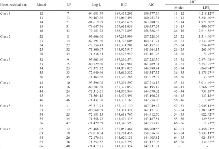
The phenotypic and animal permanent environmental variances displayed similar behavior, increased in the first week, decreased from 7 to 14 days and increased again until 35 days of age due to scale effect, since the weights increased with age. However, animal permanent environmental variance displayed lower values (Figure 1).
Similar results were reported by Akbas et al. (2004), Dionello et al. (2008) and Bonafé et al. (2011), while studying meat quails, in which both variances also increased with age.
Additive genetic variance increased from birth to 35 days of age and dropped slightly in the last week. The
residual variance also decreased at 21 and 35 days of age; however, it increased up to 42 days of age. The drop of additive genetic variance at 42 days of age may be related to animal behavior patterns, since they become more agitated in the last rearing stages, females reach sexual maturity and males develop competitive behavior to determine patterns of social dominance, such as competition for territory, food and water. These factors may lead to an increase in residual variance that possibly reflects on the declining additive genetic variance.
Heritability decreased along the growth rate curve, ranging from 0.51 (1 day) to 0.16 (42 days of age). These results contradict Bonafé et al. (2011), who reported that heritability decreased up to 14 days, increased from 14 to 35 days and decreased again after 35 days (Figure 2).
According to Akbas et al. (2004), the heritability estimated for body weight of meat quails increased until the 5th week (0.61), with a slight drop during the last week (0.44), but remained high. Dionello et al. (2008) reported increasing heritability from birth (0.01) to 42 days of age (0.50) for the EV1 lineage, but low values (0.01 to 0.10) for the EV2 lineage.
Silva et al. (2010), while studying meat quails using multiple trait model, also reported that estimates decreased as age increased, varying from 0.43 at 28 days to 0.27 at 147 days of age.
The downward trend in heritability from 35 to 42 days may be related to the increase of the residual variance in the last two weeks, in which caused a steeper decrease of the additive genetic variance.
Estimates of genetic correlations (Table 4) between weights at different ages were high and positive, except for the correlation between birth weight and life weight, thus suggesting that selection should not be based on birth weight. From 7 days of age, all genetic correlations between body weights were high and positive, indicating that selection can start at this age. The highest genetic correlation (0.972) was observed between 21 and 28 days of age, suggesting that selection at 28 days of age can be effective, considering that correlation between 28 and 35
Table 3 - Estimates of heterogeneous residual variance components (model 66) for meat quails
Variance
component Model
Age (days)
1 7 14 21 28 35 42
σ2
a 66 0.39 15.45 62.72 156.52 246.22 240.37 189.09
σ2
p 66 0.17 16.87 100.38 432.43 779.74 876.52 580.68
σ2
e 66 0.19 0.19 42.92 33.40 95.34 21.33 347.60
σ2
f 66 0.75 32.52 206.03 622.36 1,121.31 1,138.23 1,117.37
^ ^ ^ ^
σ2 a
- additive genetic variance; σ2
p - permanent environment variance; σ2e - phenotypic variance; σ2 - residual variance.f
^ ^ ^ ^
Table 2 - Estimates of variances (diagonal), covariances (below the diagonal) and correlations (above the diagonal diagonal) among random regression coefficients (b0 to b5) and the eigenvalues of the coefficient matrix for model 66
b0 b1 b2 b3 b4 b5 Eigenvalues (%) Additive genetic effect Ka = 6
b0 204.57 0.89 -0.69 -0.59 0.35 0.65 92.26 b1 92.42 52.51 -0.40 -0.74 0.03 0.64 5.65 b2 -40.07 -11.82 16.12 0.52 -0.88 0.59 2.01 b3 -20.01 -12.70 4.94 5.53 -0.27 -0.78 0.06 b4 3.42 0.14 -2.39 -0.44 0.45 0.37 0.02 b5 4.03 2.07 -1.03 -0.80 0.10 0.19 0.01
Permanent environmental effect Kp = 6
days of age (selection age) was also high (0.965). These results are consistent with those reported by Dionello et al. (2008) and Bonafé et al. (2011), who also reported high genetic correlation from 7 days of age.
The permanent environmental correlations were, in general, similar to the genetic correlations, which highlights the importance of strong permanent effect on body weight, indicating that environmental factors may influence body weight at all ages.
The genetic trend (Figure 3) displayed an increasing pattern over generations (1.2586 g/generation) for the genetic value for body weight at 35 days of age.
Figure 2 - Heritability versus age for LF1 meat quails.
0.51 0.47 0.30 0.25 0.22 0.21 0.16 0.00 0.10 0.20 0.30 0.40 0.50 0.60
0 7 14 21 28 35 42
Age (days) H e r i t a b i l i t y 4.1845 5.3915 -0.4036 10.3116 VG =2.9831+1.2586 Generation
-2 0 2 4 6 8 10 12
0 1 2 3
Generation
Genetic
value
(g)
Figure 3 - Genetic trend of breeding values for weight at 35 days of age versus generations for the growth rate curve of LF1 lineage meat quails.
Figure 1 - Components of additive genetic (σ2
a ), permanent environment (σ2p ), phenotypic (σ2e ) and residual (σ2 ) variances for weight versus f
age for meat quails.
^ ^ ^ ^ 0 50 100 150 200 250 300
0 7 14 21 28 35 42 49
Age (days) A d d i t i v e v a r i a n c e 0 100 200 300 400 500 600 700 800 900
0 7 14 21 28 35 42
Age (days) P e r m a n e n t e n v i r o n m e n t v a r i a n c e 0 200 400 600 800 1000 1200
0 7 14 21 28 35 42
Age (days) P h e n o t y p i c v a r i a n c e 0 50 100 150 200 250 300 350 400
0 7 14 21 28 35 42
Age (days) R e s i d u a l v a r i a n c e
diferentes estruturas de variâncias residuais. Revista Brasileira de Zootecnia, v.32, n.5, p.1104-1113, 2003.
FELIPE, V.P.S. Estudo da interação genótipo-ambiente em codornas de corte. 2010. 59f. Dissertação (Mestrado em Genética e Melhoramento Animal) - Universidade Federal de Minas Gerais, Belo Horizonte.
FRIDRICH, A.B.; VALENTE, B.D.; FELIPE SILVA, A.S. et al. Exigência de proteína bruta para codornas européias no período de crescimento. Arquivo Brasileiro de Medicina Veterinária e Zootecnia, v.57, n.2, p.261-265, 2005.
MEYER, K. “WOMBAT” - Digging deep for quantitative genetic analyses by restricted maximum likelihood. In: WORLD CONGRESS ON GENETIC APPLIED TO LIVESTOCK PRODUCTION, 8., 2006, Belo Horizonte. Proceedings... Belo Horizonte, [2006] (CD-ROM).
MEYER, K. Random regressions to model phenotypic variation in monthly weights of Australian beef cows. Livestock Production Science, v.65, n.1, p.19-38, 2000.
NUNEZ-ANTÓN, V.N.; ZIMMERMAN, D.L. Modelling nonstationary longitudinal data. Biometrics, v.56, p.699-705, 2000. OLIVEIRA, E.G.; ALMEIDA, M.I.M.; MENDES, A.A. et al.
Desempenho produtivo de codornas de ambos os sexos para corte alimentadas com dietas com quatro níveis protéicos. Arquivo Brasileiro de Medicina Veterinária e Zootecnia, v.7, n.2, p.75-80, 2002.
SARMENTO, J.L.R. Modelos de regressão aleatória para avaliação genética da curva de crescimento de ovinos da raça Santa Inês. 2007. 101f. Tese (Doutorado em Genética e Melhoramento) - Universidade Federal de Viçosa, Viçosa, MG.
SARMENTO, J.L.R.; ALBUQUERQUE, L.G.; TORRES, R.A. et al. Comparação de modelos de regressão aleatória para estimação de parâmetros genéticos em caprinos leiteiros. Revista Brasileira de Zootecnia, v.37, n.10, p.1788-1796, 2008.
SILVA, L.P.; LEITE, C.D.S.; SOUSA, F.M. et al. Parâmetros genéticos para pesos corporais de matrizes de codornas de corte. In: SIMPÓSIO BRASILEIRO DE MELHORAMENTO ANIMAL, 8., 2010, Maringá. Anais... Maringá, [2010]. (CD-ROM). SOUSA, J.E.R.; SILVA, M.A.; SARMENTO. et al. Homogeneidade
e heterogeneidade de variância residual em modelos de regressão aleatória sobre o crescimento de caprinos Anglo-Nubianos. Pesquisa Agropecuária Brasileira, v.43, n.12, p.1725-1732, 2008. THOLON, P.; QUEIROZ, S.A.; Utilização de diferentes estruturas
de variância residual em modelos de regressão aleatória para descrição da curva de crescimento de perdizes (Rhynchotus rufescens) criadas em cativeiro. Revista Caatinga, v.21, n.2, p.37-47, 2008.
VELOSO, R.C.; DRUMOND, E.S.C.; VASCONCELOS, R.C. et al. Proteína bruta e energia metabolizável para codornas de corte: 1 - Fase inicial. In: SIMPÓSIO INTERNACIONAL, 4.; CONGRESSO BRASILEIRO DE CODORNAS DE CORTE, 3., 2010, Lavras. Anais... Lavras, [2010]. (CD-ROM).
WOLFINGER, R. Covariance structure selection in general mixed models. Community of Statistics – Simulation, v.22, n.4, p.1079-1106, 1993.
Conclusions
The use of sixth order Legendre polynomial along with residual variance divided into six periods was the best fit for the growth rate curve of female LF1 meat quails, and they should be considered for breeding evaluation processes by random regression models. Heritability estimates decreased along the growth rate curves; therefore, genetic gains are higher when younger birds are selected. The genetic trend of breeding values increased over generations, thus symbolizing genetic progress of the studied population.
References
AKBAS, Y.; TAKMAN, Ç.; YAYLAC, E. Genetic parameters for quail body weights using a random regression model. South African Journal of Animal Science, v.34, n.2, p.104-109, 2004.
BONAFÉ, C.M. Avaliação do crescimento de codornas de corte utilizando modelos de regressão aleatória. 2008. 58f. Dissertação (Mestrado em Genética e Melhoramento) - Universidade Federal de Viçosa, Viçosa, MG.
BONAFÉ, C.M.; TORRES, R.A.T.; SARMENTO, J.L.R.S. et al. Modelos de regressão aleatória para descrição da curva de crescimento de codornas de corte. Revista Brasileira de Zootecnia, v.40, n.4, p.765-771, 2011.
CORRÊA, G.S.S.; SILVA, M.A.; CORRÊA, A.B. et al. Exigências em proteína bruta para codornas de corte EV1 em crescimento. Arquivo Brasileiro de Medicina Veterinária e Zootecnia, v.59, n.5, p.1278-1286, 2007.
DIONELLO, N.J.L.; CORREA, G.S.S.; SILVA, M.A. et al. Estimativas da trajetória genética do crescimento de codornas de corte utilizando modelos de regressão aleatória. Arquivo Brasileiro de Medicina Veterinária e Zootecnia, v.60, n.2, p.454-460, 2008. EL FARO, L.; ALBUQUERQUE, L.G. Utilização de modelos de
regressão aleatória para produção de leite no dia do controle, com
Age Age (days)
1 7 14 21 28 32 42
1 - 0.35 0.32 0.32 0.35 0.39 0.44 7 0.27 - 0.91 0.76 0.65 0.60 0.64 14 0.34 0.64 - 0.94 0.85 0.77 0.69 21 0.26 0.46 0.96 - 0.97 0.89 0.75 28 0.22 0.42 0.90 0.96 - 0.96 0.83 35 0.19 0.36 0.70 0.79 0.92 - 0.93 42 0.19 0.36 0.69 0.78 0.91 0.99