Multiproduct Firms, Firm Dynamics, and the Productive
Mix of Brazilian Manufacturing Firms
♦
Juliana Dias Alves1
Mauro Sayar Ferreira2
Abstract
This paper studies the Brazilian manufacturing sector in line with the literature on heterogeneous firm. We focus i) on the characteristics of firms that are multi-product (MP), multi-sector and multi-industry; and ii) on the analysis of their scope, including the determinants of product switching, behavior over business cycle, and relation with several firm’s characteristics. MP corresponds to 37% of all manufacturing firms, but generates 81% of the output. They employ more workers, are more likely to be exporters, have higher labor productivity and higher TFP. The extensive margin due to adding and retirement of products contributes more to output growth than entry and exit of firms. All margins are positive correlated to GDP growth: the intensive margin has an almost perfect correlation, followed by the product margin, with values around 0.91, and then by firm’s margin, with correlations around 0.60. When restricting the study to continuing firms, it was found that half of the annual output growth (from 2005 to 2009) was originated by firms that switched products. Those that have net added (dropped) items had higher (smaller) increase in output, in employees, and in the TFP. Having higher TFP, more employees, or being an exporter increase the probability of only adding or only dropping items in the future.
Keywords
Multiproduct. Scope. Total factor productivity. Heterogeneous firms. Extensive margin. Intensive margin. Export.
Esta obra está licenciada com uma Licença Creative Commons Atribuição-Não Comercial 4.0 Internacional. ♦ This work is part of the Doctoral thesis of Juliana Dias Alves, defended in 2015 at the
Universi-dade Federal de Minas Gerais. We would like to thank Naércio Menezes, Mauro Rodrigues Jr., and the anonymous referee for valuable comments and suggestions. We also thank Antonio Braz for his valuable help on how to deal with the dataset and several other discussions. As usual, all errors are our own fault.
1 Economista – Instituto Brasileiro de Geografia e Estatística (IBGE)
Endereço: Rua Oliveira, 523 – Cruzeiro – Belo Horizonte/MG – Brasil – CEP: 30310-150 E-mail: juliana.alves@ibge.gov.br – https://orcid.org/0000-0003-3236-2762
2 Professor – Universidade Federal de Minas Gerais (UFMG)
Endereço: Av. Antonio Carlos, 6627 – Pampulha – Belo Horizonte/MG – Brasil
Resumo
Este artigo analisa a indústria manufatureira no Brasil na perpsectiva da literatura de firmas heterogêneas. A análise focou i) nas características das firmas multi-produto (MP), multi-setor e multi-indústria; e ii) no escopo das firmas, incluindo os determinantes da alteração de produtos, comportamento ao longo do ciclo econômico, e relação com demais características de cada empresa. Firmas do tipo MP representam 37% do total, mas geram 81% do valor da produ-ção (VP). Elas empregam mais funcionários, têm maior probabilidade de serem exportadoras, maior produtividade do trabalho e maior produtividade total dos fatores (PTF). A margem extensiva proveniente da adição e retirada de produtos do leque produtivo contribui mais para o crescimento do VP do que o movimento de entrada e saída de firmas do mercado. Todas as margens correlacionam-se positivamente com o crescimento do PIB: a margem intensiva apresenta correlação quase perfeita, seguida pela margem de produto, com valores em torno de 0,91, e depois pela margem das firmas, cuja correlação ficou em torno de 0,60. Ao analisar as firmas sobreviventes, metade do crescimento do VP (de 2005 a 2009) teve origem naquelas que promoveram algum tipo de alteração no escopo produtivo. As firmas que adicionaram (retiraram) produtos ao (do) leque de produção obtiveram maior (menor) crescimento do VP, do número de empregados e da PTF. Firmas com maior PTF, com mais trabalhadores e as exportadoras têm maior probabilidade de somente adicionar ou somente retirar produtos do seu escopo produtivo.
Palavras-Chave
Multiproduto. Escopo. Produtividade total dos fatores. Firmas Heterogêneas. Margem extensiva. Margem intensiva. Firmas exportadoras.
Classificação JEL D2. F23. L1. L16. L6.
1. Introduction
This is a pioneer study about the productive scope of the Brazilian manu-facturing sector in line with the literature on heterogeneous firm proposed mainly by Bernard, Redding and Schott (2010) [BRS (2010), henceforth], BRS (2011) and Eckel and Neary (2010). These works incorporate product heterogeneity among multiproduct plants in the set up that has been deve-loped by Melitz (2003), Bernard et al. (2003), Melitz e Ottaviano (2008), among others.
BRS (2010) added the possibility of adjustments in the productive mix inside each firm. Specifically, surviving firms can manufacture new varieties and/or drop old ones. Specializing in items they can manufactu-re momanufactu-re efficiently contribute to a better use of manufactu-resources in an economy. This product extensive margin, which we refer to as extensive margin 2 (EX2, henceforth), has not deserved the appropriate attention previously, despite the fact that approximately 50% of U.S. manufacturing firms con-ducts some change in scope within at least a 5-year interval (BRS, 2010).
Main Results
From 2005 to 2009, only 37% of the firms in the Brazilian manufactu-ring sector were multiproduct, but they were responsible for 81% of total output. They employed more workers, were more likely to be exporters, had higher labor productivity and higher total factor productivity.
Using a product decomposition proposed by BRS (2010), an average of 86% of aggregate output was due to products manufactured by the same firm (intensive margin) in previous period; 8.5% from varieties produced by surviving firms that did not produce the item in previous year (EX2); and the remaining 5.5% from the traditional extensive margin (EX1).
The literature still lacks a good body of stylized facts regarding the busi-ness cycle contribution of these margins. By decomposing the output gro-wth through the years new evidences were provided to help in this direc-tion. The intensive margin contributed with 76.2% of the output increase from 2005 to 2009; product margin from established firms with 14.9%, and traditional extensive margin (EX1) with 8.9%. During the financial crisis of 2008/2009, the total output fell by 15.88%: variation in the in-tensive margin was -15.31%, in EX2 was -0.05%, and in EX1 was -0.52%.
Since we were particularly interested in studying firms that changed sco-pe, the entire section 6 was dedicated to analyze surviving firms. Among this group, 62.7% promoted at least one change in the productive scope from 2005 to 2009, contributing with 73.4% of the total output divided as follows: 47.4% by firms that added and dropped varieties, 13.9% by those that only added, and 12.1% by only droppers. Exporters contributed more to output among surviving firms. Exporters and larger firms (top decile in terms of output) were more likely to modify scope.
Evaluating the output growth among surviving firms, in a similar exercise conducted by Navarro (2012) for the Chilean manufacturing sector, it was found that approximately 50% of product increase was generated by firms that conducted some change in the productive mix. Among them, the most important contribution came from firms that manufactured more items.
The last exercise aimed at verifying the determinants of changes in scope among surviving firms. Larger firms (by number of employees) and expor-ters were more likely to either add or drop items from their productive mix, compared to those that did not modify their scope. Firms with higher TFP were less likely to only add or only drop varieties.
Related Literature
The theoretical development of BRS (2010), BRS (2011) and Eckel and Neary (2010) adds, to the heterogeneous firm environment, multiproduct plants and consumers with stronger preference over some varieties, which allow demand shocks to influence results. Given preferences, most pro-ductive firms would produce more varieties since they can afford paying for fixed costs associated to the production of each extra item. According to BRS (2010), this prediction of the model helps to explain the stylized fact that most productive plants tend to produce more varieties.
for existing products. The continuum of varieties would be supplied by several firms, each having a “core competence” in which certain products would be manufactured more efficiently. The further away from this cen-ter, the higher the marginal cost to produce the item. The productive mix would then depend on the degree of competition for each item, on consumers’ preference, and on the relation between “excellence core” and marginal cost of each variety. International competition may then result in higher aggregate TFP by forcing firms to produce varieties closer to their competence core, but can also result in fewer items produced by a country.
BRS (2011), based on Mayer, Melitz e Ottaviano (2010), also shows that multiproduct firms would tend to obtain higher revenue from items closer to their excellence core, since productivity and quality would decline as new varieties are manufactured. Arkolakis and Muendler (2010) further observed that, in the presence of entry cost per each new variety supplied, larger and more efficient plants would produce more output and varieties, resulting in positive correlation between extensive and intensive margins within a firm.
Nocke and Yeaple (2006) do not use the notion of competence core of products, but allow firms to have distinguished organizational capacity, which determines the rate at which the marginal cost of an extra va-riety increases. Better managerial skills would result in smaller marginal cost, implying greater variety. In line with these theoretical predictions, Iacovone and Javorcik (2010) documented, for Mexico, that products more distant from the excellence core had higher probability of being dropped from the productive mix following the country’s entry in NAFTA.
Besides this introduction, the rest of this work is organized as follows. Next section presents data and explains the procedures to allow com-bining two microdata record we work with: Annual Survey of Industry - Product (PIA Product), and the Annual Survey of Industry – Enterprise
(PIA Enterprise).1 Section 3 characterizes data according to the
contribu-tion of each item to output according to the amount of varieties produced by each group of firm. We also show the relevance of MP, MI, and MS firms, in terms of their presence and their contribution to production. In section 4 we are able to empirically corroborate some predictions of BRS (2010, 2011) and Eckel and Neary (2010) by verifying differences bet-ween MP, MI, and MS against their single counterparts. Later, in section 5, we decompose production and analyze the contribution of the intensive margin and two extensive margins to output production and output gro-wth. Correlation between these margins’ growth rate and NIPA aggregates growth rates is also estimated, generating interesting business cycle styli-zed facts. Section 6 studies only surviving firms in an attempt to focus on their strategies towards productive mix and how such strategies are related to firm’s performance. Section 7 concludes.
2. Data
Our work was only possible because we connected, at firm level, two different surveys conducted by the Brazilian Institute of Geography and Statistics (IBGE). The first, called Annual Survey of Industry-Product (PIA-Product), surveys the plants of every manufacturing firm with 30 or more employees and/or that had gross revenue above a certain thre-shold in the preceding year of the survey. For each firm, it informs the amount produced, production value, and revenue from each product and
1 Important to mention that Esteves (2015) has also conducted a study for Brazil using
service. These products and industrial services, which encompass around 3,500 different items, were classified according to the List of Industrial
Products 2 (PRODLIST-Industry), following the Common Classification of
MERCOSUR (NCM), and presented by classes of the National Standard Industrial Classification of All Economic Activities (CNAE 2.0). PIA-Product started in 1998, but microdata only became available as of 2005.
Table 1 - Number of products in 2005 and 2009, absolute variation, and number of industries in 2009. According to four digits CNAE 2.0
Sector N.º products
(2005)
N.º products (2009)
Absolute variation
N.º industries (2009)
Food products 301 310 9 31
Beverages 29 28 -1 5
Tobacco products 7 7 0 2
Textiles 138 147 9 14
Wearing apparel 87 89 2 6
Leather and related products 69 71 2 8
Wood, products of wood and cork, except furniture; articles
of straw and plaiting materials 44 44 0 5
Paper and paper products 84 87 3 9
Printing and reproduction of recorded media 41 52 11 6
Coke and refined petroleum products 38 40 2 5
Chemicals and chemical products 445 439 -6 25
Basic pharmaceutical products and pharmaceutical
preparations 95 89 -6 4
Rubber and plastics products 114 118 4 7
Other non-metallic mineral products 113 111 -2 11
Basic metals 105 113 8 14
Metal products, except machinery and equipment 196 199 3 16
Computer, electronic and optical products 154 161 7 11
Electrical equipment 133 133 0 10
Machinery and equipment n.e.c. 368 374 6 26
Motor vehicles, trailers and semi-trailers 82 84 2 10
Other transport equipment 51 55 4 10
Furniture 69 70 1 4
Other manufacturing 132 139 7 9
Repair and installation of machinery and equipment 39 54 15 10
Total 2934 3014 80 258
Source: PIA-Product and PIA-Enterprise (IBGE).
2 PRODLIST-Industry is a classification used by the Brazilian Institute of Geography and Statistics
The second database is the Annual Survey of Industry – Enterprise (PIA-Enterprise). It provides information about the number of employees, wages and salaries, revenue and expenses, production cost and gross value added. The survey unit corresponds to enterprises with 10 or more employees and/or whose gross revenue surpassed a certain threshold in the previous year of the survey. The period ranging from 1996 to 2007 was originally classified according to the previous industrial classification, CNAE 1.0.
From 2007 to 2009,3 classification was according to CNAE 2.0. Since
our estimates use data from before and after 2007, the correspondence between both classifications were investigated and every pre-2007 product information was recoded according to CNAE 2.0.
So, while PIA-Product provides a panel of firms with the production value of each product and service, classified according to the Prodlist, PIA-Enterprise characterizes several dimensions of each firm at four digits CNAE. The connection of both surveys allows analysis at firm and product level.
Production value of each item was deflated by a specific price index. These deflators were obtained from the Supply and Use Tables (TRU), which is part of the System of National Accounts (SNC), after establishing
a correspondence between activities in SNC and CNAE 2.0.4
Table 1 provides a summary of sectors, industries, and products. A total of 3,014 items were produced in 2009 and 2,934 in 2005. In absolute terms, larger increases in the number of varieties were observed in the following sectors: food products (10), textiles (13), printing and reproduction of recorded media (18), basic metals (24), repair and installation of machi-nery and equipment (33).
3. Characterizing the Data
We started characterizing the data by verifying how the production val-ue is distributed among varieties produced by each firm. Table 2 pres-ents the average share of revenue originated by each good after
control-ling the number of varieties produced.5 The columns show the number
of varieties manufactured by a firm, which can be 1, 2, and so on. Any firm producing 10 or more goods was pooled in the last column (≥ 10). A specific row informs the average contribution of a product to the total revenue of a “representative” firm producing the number of items indi-cated in the specific column. For instance, among firms producing only 2 items, the contribution of a single good for the total revenue was, on average, 75%, while the remaining 25% would come from the second good. Firms producing 9 items concentrate, on average, 45% of their revenue on only one item and another 20% on a second variety. The remaining 35% is divided among the other 7 products, also in a disproportionate manner.
As comparison, BRS (2010) reported that US manufacturing firms pro-ducing only two goods, had, on average, 80% of the revenue generated by one of them, against 75% we found for Brazil. They also verified that among those producing 10 or more items, the average contribution of the main product was 46%, almost identical to the 45% we observed for Brazil. These results are also very similar to the patterns reported by Goldberg et al. (2010), Navarro (2012) and Söderbom and Weng (2013), when analy-zing Mexico, Chile and China, respectively.
The overall finding for Brazil is that, on average, few items contribute with a very large fraction of the total output of each manufacturing firm. This is in line with the developments of BRS (2010) and Eckel and Neary (2010) for whom each firm has better performance in products closer to their excellence core, resulting in a distribution of revenue skewed in a way that some varieties are responsible for a greater share of the revenue.6
5 The variable used was output value, taken from PIA-Product.
6 Nocke and Yeaple (2006) provide a different perspective: there are not differences within a firm
Table 2 - Average share (%) in output originated by each good given the number of varieties produced. Period: 2005 and 2009
Importance rank in output
production
Number of varieties produced by each firm
1 2 3 4 5 6 7 8 9 ≥ 10
1st 1.00 0.75 0.64 0.58 0.54 0.50 0.49 0.46 0.45 0.45
2nd 0.25 0.25 0.24 0.23 0.22 0.21 0.21 0.20 0.20
3rd 0.11 0.12 0.12 0.12 0.12 0.12 0.12 0.12
4th 0.06 0.07 0.08 0.08 0.08 0.08 0.08
5th 0.04 0.05 0.05 0.05 0.06 0.05
6th 0.03 0.03 0.04 0.04 0.04
7th 0.02 0.02 0.03 0.03
8th 0.01 0.02 0.02
9th 0.01 0.01
10th 0.01
Source: PIA-Product (IBGE), 2005 and 2009. Authors' computation.
In Table 3 we report general information about the composition of ma-nufacturing firms according to their classification as multiproduct (MP),
multi-industry (MI) and multisector (MS), in 2009.7 These classifications
followed BRS (2010). Single product (SP) firms are those whose range of products falls within a single five-digit category in Prodlist. Multiproduct (MP) is one whose product range is wide enough to span several five-digit of Prodlist categories. Multi-industry (MI) has products classified in more than one CNAE in four digits, while multisector (MS) has products in more than one division (two digits of the CNAE).
Despite differences in dates and product classification, we also re-port information for countries in which similar exercise has been
conducted8 (EUA, India, Chile, Japan and China). Panel A reveals that
37% of Brazilian manufacturing firms produced more than one variety in 2009, 23% operated in more than one industry and 13% in more than one sector. The USA came closer regarding MP, with 41% of the firms produ-cing more than one variety.
7 We decided to report results for the last year available at the time this work was being elaborated.
However, values for 2005, 2006, 2007 and 2008 are all very similar.
Panel B shows that MP firms were responsible for 81% of the output, a proportion similar to those reported for India and Japan. Panel C shows the average number of product per MP firm, the average number of indus-try each MI firm participates, and the average number of sectors each MS firm belongs to. Brazilian MP firms produced, on average, 3.8 items each, close to Chile (3.9) and the US (4.0). Each MI firm belonged to an average of 2.9 industries, and each MS firm participated, on average, in 2.4 sectors.
Table 3 - The relevance of firms MP, MI, and MS: percentage of firms, contribution to output, average number of varieties, industry, and sector: USA, India, Chile, China, Japan, and Brazil
Type of firm USA India Chile Japan China Brazil Panel A – Percentage of firms (%)
MP 41 47 52 41 47 37
MI 29 33 22 31 34 23
MS 13 24 9 17 9 13
Panel B – Contribution to Output (%)*
MP 91 80 56 78 50 81
MI 87 62 23 70 43 70
MS 76 54 8 51 25 50
Panel C – Average number of items, industries and sectors
MP 4.0 3.1 3.9 2.7 2.8 3.8
MI 3.1 2.0 2.6 2.9 2.3 2.9
MS 2.5 1.7 2.2 3.1 2.1 2.4
Source: PIA-Product (IBGE), 2009. Other countries: see literature review in the introduction.
* The variable used for this analysis varies among articles. In our case we used the output value informed in PIA- Product, 2009.
4. Differences between Multiproduct, Multi-industry, and Multisector
Let Zji be a specific characteristic of firm j belonging to sector i. We want
to verify whether characteristic Z is correlated to the fact that a firm
is MP, MI and MS. These comparisons are carried after estimating the regression model
j i h ji
ji D F
Z
(1)and testing
H
0:
µ
=
0
againstH
1:
µ
≠
0
. In the previous equation, h in-dexes firm’s characteristic:h
SP,MP,SI,MI,SS,MS
.Dhji is a dummyvariable such that h
ji
D =1 if h
MP,MI,MS
and h jiD =0 otherwise.
i
F
is a fixed effect for each sector, andε
j captures randomcharacter-istics of firm j which are independent across firms. For each pair of
pos-sibility (SP or MP; SI or MI; SS or MS), one regression is estimated. We considered the following characteristics: Z = {logarithm of output value, logarithm of number of employees, a dummy that equals 1 in case a firm is an exporter and 0 if not, labor productivity,9 logarithm of the total factor productivity (TFP)10}. Results are in Table 4.
Positive and significant μ was verified in all cases, indicating that MP,
MI and MS have, on average, higher values of all variables Z when
con-trasted to SP, SI, SS, respectively. These results corroborate theoretical predictions. Specifically, when confronted against SP, it was verified that MP firms produced, on average, 8% more output value, and employed 10% more workers that were 4% more productive. They also had higher TFP.
Compared to SI firms, MI generated, on average, 6% more output, em-ployed 8% more workers that were 3% more productive. Confronting against SS firms, MS generated 4% more output and employed 6% more workers who were 2% more productive. In all cases, TFP was higher in
MI and MS.11
9 Labor productivity is measured as the logarithm of output per number of employers.
10 TFP of each firm was estimated from 2005 to 2009 according to Olley and Pakes (1996) and
Levinsohn and Petrin (2003). For more details, see the appendix and Alves and Ferreira (2013).
11 Our results are difficult to compare to those of Esteves (2015), since the author did not analyze the
Table 4 - Relationship of MP, MI, and MS with output, number of employees, exporting status, labor productivity, and TFP. Brazil, 2005-2009
Characteristics MP MI MS
Ln(output) 0.08*** 0.06*** 0.04***
Ln(n.employees) 0.10*** 0.08*** 0.06***
Exporter (1 if yes) 0.23*** 0.19*** 0.14***
Ln(output/employee) 0.04*** 0.03*** 0.02***
Ln(TFP) 0.00 ** 0.00 ** 0.00 **
Source: PIA-Product (IBGE), 2005 and 2009. Authors’ computation.
Note: Reported values correspond to estimated coefficient μ of Equation 1: i j h ji ji D F Z . Characteristics in the 1st column correspond to variables Z. F
i are sector fixed effects. Significance: ***
1%, ** 5% and * 10%. Number of observations: 159,717.
Regarding their presence in the international market, MP was 23% more likely of being an exporter than SP. MI had 19% higher probability of being an exporter than SI, and MS was 14% more likely to be and exporter than SS.
5. Output Decomposition: Extensive and Intensive Margin
We have just verified that, in 2009, 81% of the output was generated by MP firms. Next, the relevance of the intensive margin, product mar-gin (EX2) and plant marmar-gin (EX1) in total production and in production growth is assessed.
5.1. Contribution to Output
We follow Bernard and Okubo (2013) who suggested decomposing the output of each product by the type of firm producing it. This allows veri-fying the proportion of output due to each margin.
Let’s consider Yp,t/t-h as the production of good p at time t according to firm’s status in t-h. A firm producing Y at time t could have been of any following type in t-h: a surviving firm that produced good p in t-h and in
t (group B); a surviving firm that added Y to the production mix at time
t (group N). Considering j as the index of an individual firm, this decom-position can be represented as follows:
∑
∑
∑
∈ − ∈ − ∈ − −=
+
+
p pp j N
j h t t p A j j h t t p B j j h t t p h t t
p
Y
Y
Y
Y
,/ ,/ ,/ ,/ (2)In a second decomposition, the production of p at time t was divided according to the firm’s status at t+h (Yp,t/t+h). As previously, a surviving firm manufacturing Yp at t and t+h belongs to B. A surviving firm
produ-cing Yp in t but no longer in t+h belongs do D. Firms manufacturing Yp at
t but that left the market in t+h12 belong to group X. This decomposition works as follows:
∑
∑
∑
∈ + ∈ + ∈ + +=
+
+
p pp j X
j h t t p D j j h t t p B j j h t t p t h t
p
Y
Y
Y
Y
, / ,/ ,/ ,/(3)
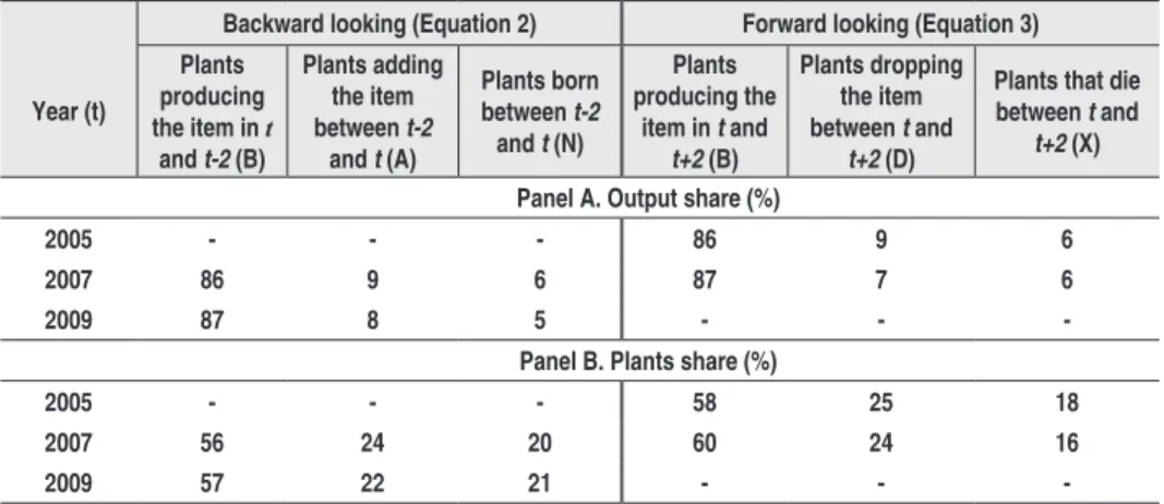
Columns 2 to 4 of Table 5 report the backward decomposition (Equation 2), while the last three columns inform the forward decomposition (Equation 3). Panel A presents the share of each group in aggregate output, while panel B shows the proportion of firms in each group. We considered
years 2005, 2007 and 2009, so that h=2.
Backward (forward) results indicate that 86-87% of the output was
ge-nerated by products manufactured by the same firm in t-2 (t+2). Items
produced by continuing firms that have added (dropped) them were res-ponsible for 8-9% (7-9%) of the total output, slightly superior to items
made by new firms (5-6%) or by those that died (6%).13 Our results are
very similar to those of Bernard and Okubo (2013) for Japan.
In Panel B the proportion of firms belonging to each group is verified. Around 58% belonged to B, producing the same product in two consecu-tive years. Surviving firms that added and dropped products represented 22%-25% of the firms investigated. Inexistent firms and those that left the market ranged from 16% to 21% of the total.
12 These decompositions have the advantage that results can be easily transformed into percentage
variations, with no need for deflating.
13 One can argue that entrants may arrive with enormous innovation potential and may become major
Table 5 – Product-Level Decomposition of output: 2005, 2007 and 2009
Backward looking (Equation 2) Forward looking (Equation 3)
Year (t)
Plants producing the item in t
and t-2 (B)
Plants adding the item between t-2
and t (A)
Plants born between t-2
and t (N)
Plants producing the
item in t and t+2 (B)
Plants dropping the item between t and
t+2 (D)
Plants that die between t and
t+2 (X)
Panel A. Output share (%)
2005 - - - 86 9 6
2007 86 9 6 87 7 6
2009 87 8 5 - -
-Panel B. Plants share (%)
2005 - - - 58 25 18
2007 56 24 20 60 24 16
2009 57 22 21 - -
Source: PIA-Product (IBGE), 2005, 2007, and 2009. Authors’ computation.
Note: The first three columns show decomposition according to
∑
∑
∑
∈ − ∈ − ∈ −− = p + p + jNp j h t t p A j j h t t p B j j h t t p h t t
p Y Y Y
Y ,/ ,/ ,/ ,/ , where Yp,t/t-h is the production
of good p at time t according to firm’s status in t-h. Each firm j producing product p at time t has status B, A or N, whose definitions are in the top of each column. The last three columns decompose products according to
∑
∑
∑
∈ + ∈ + ∈ ++ = p + p + jXp j h t t p D j j h t t p B j j h t t p h t t
p Y Y Y
Y,/ ,/ ,/ ,/ , where Yp,t/t-h is the production of
good p at time t according to firm’s status in t+h. Each firm j producing product p at time t has status B, D or X, whose definitions are at the top of each column.
5.2. Contribution to Growth
The decomposition suggested by BRS(2010) was conducted next in order to verify the contribution of each margin to the total output gro-wth. Variation in output from year t-h to year t (
∆
Y
t) could be due to: (i) two extensive margins, the first resulting from net entry of new firms (EX1, plant margin), and the second from net addition of items by conti-nuing firms (EX2, product margin); and (ii) the intensive margin (INT) determined by net growth in the output of items already produced by continuing firms. Bj i S ijt iG ijt i A ijt i D ijt X
j jt N
j jt
t Y Y Y Y Y Y
In Equation 4, j indexes the following status: new firm (N), firm that left the market (X), or a surviving firm (B). The terms
∑
j∈N∆Yj t and∑
j∈X∆Yj t capture, respectively, variation in output arising from new firmsand exit of old ones. Their net effect represents plant extensive margin EX1. Surviving firms (B) are divided in four groups indexed by i = {S, G, A, D}. Terms
∑
i∈S∆
Y
ijt and∑
i∈G∆
Y
ijt capture, respectively, old itemsproduced by established firms whose output has either declined (i=S) or
increased (i=G). Their net effect corresponds to the intensive margin.
The last two terms inside brackets,
∑
i∈A∆
Y
ijt and∑
i∈D∆
Y
ijt, capture, respectively, variation in output due to adding and dropping of items by continuing firms. Their net effect corresponds to the product extensive margin EX2.Decomposition of output variation according to Equation 4 is presented in Table 6. The last row shows the percentage variation from 2005 to 2009. Previous rows show variation in year t against t-1, starting from t=2006.14 The second column informs the total output growth. The remaining col-umns show output growth of each group according to the decomposition proposed by Equation 4.
The last row reveals that output increased by 27.54% from 2005 to 2009. The plant extensive margin 1 (EX1) was responsible for 2.45%, while sur-viving firms throughout these years (group B) contributed with 25.09%: 20.99% originated in the intensive margin, and 4.10% in extensive margin
2 (EX2).15 In sub periods, EX1 only delivered results better than those
of EX2 in 2007, when growth from EX1 was 11.47%, against 1.22% from EX2.
Overall, our results are in line with those reported for most countries: intensive margin contributing far more to output growth, followed by
product margin and, lastly, by firm’s margin.16 This superiority of the
intensive margin should not really surprise. Once the production of a spe-cific item is already in place, it is easier for a firm to respond to stimulus in either direction. It could, for instance, more easily expand production by using more hours as a response to higher demand. Logistics to supply
14 Since we are interested in real variation, nominal values of each product were deflated by the
appro-priate four digit deflator of CNAE in accordance to the Brazilian National Account System. Given the nature of the decompositions presented in Table 7, deflating was not necessary.
15 These results are almost identical to those reported by BRS(2010) for the USA from 1992 to 1997. 16 An exception was the study of Navarro (2012) for Chile, who reported the product margin coming
this extra amount would be an easier task to solve compared to an en-trant’s situation. Better network through the entire chain also facilitates adjustments through the intensive margin.
Table 6 – Decomposition of output growth (%): 2005 to 2009
Period Total Plant Entry andExit (EX1) Intensive Margin: produce more or less of existing items Product Add andDrop (EX2)
Net Entry Exit Net More Less Net Add Drop
2005-2006 6.64 -0.71 4.29 -5.00 7.04 17.33 -10.29 0.32 6.06 -5.74
2006-2007 25.15 11.47 13.64 -2.17 12.46 19.59 -7.12 1.22 6.35 -5.13
2007-2008 17.89 0.52 2.22 -1.70 16.63 22.27 -5.64 0.74 5.02 -4.28
2008-2009 -15.88 -0.52 3.83 -4.35 -15.31 9.43 -24.75 -0.05 4.89 -4.94
2005-2009 27.54 2.45 11.73 -9.28 20.99 29.51 -8.52 4.10 13.25 -9.15
Notes. Table reports output growth decomposition in extensive margin due to entry and exit of firms (EX1), due to intensive margin and due to extensive margin of surviving plants that add and retire pro-ducts (EX2).
Similar arguments may justify the product extensive margin (EX2) as second in determining total output variation. Compared to the firm’s ex-tensive margin (EX1), implementing adjustment in the production mix seems an easier task once a firm’s internal structure (lawyers, accountants, managers etc.) is already set up. As an example, a continuing firm could benefit from existing networks and logistics, which would have to be built from scratch in the case of an entrant. Response to external stimulus should then happen more rapidly and less costly for incumbents (either by adjusting production or changing the mix).
The importance of the product margin can be better assessed if its con-tribution to growth is considered in relative terms. The net growth of the intensive margin represented 76.2% of the aggregate increase from 2005 to 2009 (20.99% out of 27.54%). The product margin contributed with 14.9% for the aggregate growth (4.90% in 27.54%), which is a considerable amount since we are not simply talking about adjusting the volume of an already produced item.
new items.17 These numbers imply that 31% of total (gross) increase in output of established firms was due to the production of new varieties. What makes the net contribution of the product margin smaller is the similar high proportion of retirement of items, which, on the other hand, opens space for the introduction of new varieties, especially if a firm is not willing to incur in profound and (sometimes) costly investments in order to have a new product in the production mix.
The fact that the firm's margin contributes least to output growth should not surprise, since it is in line with the findings reached by similar research on other countries. The real surprise is the lack of attention the product margin, which comes second in relevance, has received from the profession.
5.3. Production Growth Decomposition and the Business Cycle
The behavior of each margin over business cycles is another theme not explored by the profession. Little (if nothing) is known about this rela-tion. In order to advance in this area, we bring some preliminary stylized facts based on the correlation between the annual growth rate of the Brazilian GDP and two of its components (manufacturing and investment) against the growth rate of each source of output growth in manufacturing, according to the decomposition presented in Table 6. It is worth empha-sizing that this exercise does not intend to bring definite stylized facts, since correlations are computed based solely on 4 data points (from 2006 to 2009). Despite this limitation, the exercise is a good starting point to think how each margin behaves over cycles.
Correlations are presented in Table 7.18 The first thing to observe (in
column 2) is the almost perfect positive correlation between the total net effect (
∆
Y
t) and all three GDP variables, the highest being with themanufacturing GDP (0.996).19 Since most of the total net effect was due
to changes in the intensive margin, it is not surprising it had an almost perfect correlation with NIPA measures.
17 As a comparison, the output from new firms generated growth of 11.73% (see Table 6). 18 Figures A1, A2, and A3 in the appendix allow visualizing the evolution of some NIPA growth measures
(in the right scale of each plot) against the growth rate of each margin (in the left scale of each plot).
19 That this correlation is almost 1 is also a relief, as it indicates a well conducted treatment given to
In accordance to the view that it is easier for an established firm to follow short run cycles (through intensive and/or extensive margins), correla-tions of the net EX2, which are all above 0.89, are much higher than those of the net firm margin (EX1), which range from 0.526 to 0.647. The portion of each margin responsible for generating positive effect in the output keeps a similar pattern, with the intensive margin presenting very high correlations with GDP measures (all above 0.92), followed by
the addition of products by continuing firms (column EX2 add, in Table
7). Correlations against the positive effect caused by firm entry (column
EX1 entry) were the smallest.
Looking at the negative effects, we again observe very high correlations (minimum of 0.962) between the intensive margin and the GDP
aggrega-tes (column INT less). This indicates that when GDP grows stronger, the
negative effect becomes milder (less negative). The high correlation seems in accordance to the view that it is easier for a continuing firm to make adjustments mainly by dimensioning the output of already produced items. The output variation arising from dropping items from the production
mix (column EX2 drop) has an almost zero correlation against GDP and
manufacturing GDP, being only a little higher (at 0.237) when confronted to the investment. These low correlations may indicate that the decision to drop products is a more strategic move, and, as such, should not be extremely impacted by short run cycles. On the other hand, the negative
effect arising from firms’ margin (EX1 exit) should be expected to
corre-late positively with cycles, since bad economic moments imply higher firm mortality. The numbers confirm this view since the estimated correlations ranged from 0.643 to 0.743.
Table 7 – Correlation between annual growth rate of GDP and its components against growth rate in different product decomposition. Period: 2006-2009
Variables
Net Effect Positive Effects Negative Effects
Total EX1 net
INT net
EX2 net
EX1 entry
INT more
EX2
add EX1 exit INT less EX2 drop GDP 0.993 0.608 0.964 0.915 0.490 0.940 0.636 0.643 0.974 0.056
GDP manuf. 0.996 0.647 0.952 0.934 0.528 0.928 0.644 0.661 0.962 0.064
GDP invest. 0.983 0.526 0.985 0.894 0.366 0.981 0.472 0.743 0.983 0.237
6. Surviving Firms
This last section focuses only on surviving firms. The reason for this cutoff lies on the fact that they are responsible for the product extensive margin (EX2), which we want to study more carefully.
We initially take a picture and verify the proportion of firms according to actions towards scope, conditioning on some characteristics (panel A of Table 8). The distribution according to the output generated by surviving firms (panel B of Table 8) is also verified. Following BRS (2010), there are four mutually exclusive possibilities regarding changes in the productive mix: (i) “no change”, when a firm does not add nor retire any variety; (ii) “drop”, when at least one product is taken out of the production mix; (iii) “add”, when at least one new item is incorporated to the production mix; and (iv) “both”, for adding and dropping at least one product.
Panel A of Table 8 shows the percentage of firms enrolled in each action. In the second column (“Total”) we see that only 37.3% have not changed the productive mix. The remaining 62.7% was distributed as follows: 9.2% added at least one product, 8.9% dropped at least one product, and 44.6% added and dropped at least one variety.
Table 8 - Share of firms and output, among surviving firms, according to action towards scope and characteristics: MP, MI, MS, exporting status, and size. Period: 2005-2009
Action regarding scope Total MP MI MS Exporters (X)
Non exporters
(NX)
10% larger*
Panel A: Share of firms
None 37.3 13.2 9.3 7.9 32.5 39.7 28.7
Add product(s) only 9.2 17.1 16.1 15.2 11.8 7.9 14.4
Drop product(s) only 8.9 16.5 14.8 14.1 11.4 7.6 12.9
Both:added and dropped 44.6 53.1 59.9 62.7 44.4 44.8 44.1
Panel B: Share of output (of the specific group of each column)
None 26.6 14.9 9.8 7.7 24.4 37.8 18.8
Add product(s) only 13.9 16.7 16.4 12.9 14.5 11.2 13.6
Drop product(s) only 12.1 14.5 12.9 15.7 12.0 12.4 11.1
Both: added and dropped 47.4 53.9 60.9 63.6 49.1 38.7 56.4
Notes. *With respect to output value. Columns add to 100%.
Regarding participation in external market, non-exporters were more li-kely to leave their mix unchanged: 39.7% compared to 32.5% among ex-porters. In the opposite direction, the fraction of those that have only added or only dropped product(s) was higher among exporters: respecti-vely, 11.8% and 11.4% against 7.9% and 7.6% for NX. There was basically no difference between the proportion of firms conducting both actions: 44.4% for X and 44.8% for NX. Firms belonging to the top decile (with respect to output value) were less likely to keep steady their production mix (28.7%) when compared to all firms together (37.3%). Larger compa-nies were more likely to add new products (14.4% against 9.2%) and retire old ones (12.9% against 8.9%). No substantial difference was found in the proportion of firms conducting both actions.
Panel B informs the contribution of each action group for the aggregate
output among surviving firms from 2005 to 2009.20 Those 37.3% that
did not change scope were responsible for only 26.6% of the output. The remaining 62.7% that modified the mix were responsible for 73.4% of the output which was distributed as follows: 13.9% generated by firms that only added products, 12.1% by droppers, and 47.4% by firms doing both.
20 One should be cautious for not directly comparing the results of the product decomposition
It is clear that an average firm that promotes changes in the production mix contributes far more to aggregate output than a standard one that
does not. But this conclusion, well pictured by comparing the “Total”
column of panels A and B (Table 8), does not seem to be caused by firms being MP, MI, or MS. Export status and firm size are where big diffe-rences in panels A and B reside. Starting with size, while 28.7% of the firms belonging to top decile did not pursue any change in scope, their contribution to output was much smaller, at 18.8%. And while 44.1% of these larger firms added and dropped items from their productive mix, their contribution to output was much larger (56.4%). Similar inversion happened among exporters: 32.5% of them did not alter their mix, but these firms only contributed to 24.4% of the output in the group. The re-maining 67.5% that altered the mix contributed with 75.6% of the output among exporters.
Although nothing can be directly said regarding productivity, our results suggest that most productive firms are more likely to change scope, since the inversion just mentioned happened among exporters and larger firms, groups where higher productivity is expected. This would be in line with BRS (2010) for whom such characteristics also indicate that a firm is more likely to afford paying for product specific sunk costs.21
Overall, our results are in line with those reported for other countries: the intensive margin contributes far more to output growth, followed by pro-duct margin and, lastly, by firm’s margin. The percentage of contribution of each varies depending on the period analyzed. The profession has not even attempted to explain, neither empirically nor theoretically, what is behind the differences in these proportions across countries or even inside a country but over the business cycle.
Output and Output Growth
Although 62.7% (Table 8) of all surviving firms have conducted some type of modification in their scope (by adding, retiring, or doing both), Table 6 shows that the main source of output growth from 2005 to 2009 was the
21 BRS (2010) based their explanations using similar arguments encountered in models of firm entry
intensive margin (20.99%), followed by scope (4.10%). These results are not contradicting each other, since results in Table 8 refer to output pro-duced from 2005 to 2009, while Table 6 informs about output variation.
The high share of firms promoting modification in scope between 2005 and 2009 does not conflict with the fact that, for most of them, response to business cycles happens mostly by adjusting already produced items, which seems reasonable and expectable for at least two reasons. Firstly, it is easier and less costly to react to cycles by increasing or decreasing the amount produced of old items than by adding or retiring products. Secondly, it makes sense that a serious response to short run aggregate swings would require adjustment in the production of goods that are most important to a firm’s output. And indeed, as shown in Table 2, most of the contribution to a firm’s output tends to come from one single product, which would make it a strong candidate to suffer adjustments over busi-ness cycles.
6.1. Output Growth Performance and Scope Strategy
Results in panel B of Table 8 show association between actions in the
pro-ductive mix and output level. We are now interested in verifying whether
there is any relation between output growth and scope strategy.
Product decomposition as proposed by Navarro (2012), which is similar to the one carried out in subsection 5.2, was first performed, but now the groups are divided according to their actions towards scope. Considering
∑
j∈B∆Yj t as the output variation of a surviving firm j, between year tand t-1,22 which necessarily must have adopted only one of the following
actions indexed by
h
=
{
U
,
M
,
L
,
E
}
: kept the same productive mix, U; altered the mix and ended with more items, M; less items, L; or with thesame amount of varieties, E. Expression 6 formalizes this decomposition,
while Table 9 summarizes the results.
∑
∑
∑
∑
∑
j∈B∆
Y
jt=
h∈U∆
Y
ht+
h∈M∆
Y
ht+
h∈L∆
Y
ht+
h∈E∆
Y
ht(5)
22 Surviving firms, labeled here as group j, are the same as group B previously shown in the
Aggregate output variation among continuing firms is presented in the 2nd
column. The 3rd and 4th columns present, respectively, results for group
U and for the joined variation reached by the group of firms that pursued
any change in the productive mix (M+L+E). The last three columns
pre-sent individual results for M, L, and E, respectively. Each row informs the specific period according to the 1st column.
On average, output growth was similar in firms that did and did not change the scope. Among the first group, the largest increase was noticed among those that increased the number of varieties (M). Group L con-tributed with approximately 11% of the aggregate growth among survi-ving firms in 2007 and 2008, despite representing firms that produced less items. They however performed poorly in years of smaller aggregate output growth (2006 and 2009). Particularly during the financial crisis
(2009), the drop in output of group L was 4.61%, which represented 30%
of total contraction among surviving firms.
Table 9 – Output growth rate (%) of surviving firms and change in product mix. 2005-2009
Period
Total Surviving
(B)
No change in product mix
(U)
Changed product mix
Total (M+L+E)
More varieties (M)
Less varieties (L)
Same amount of varieties (E)
2005/2006 7.35 4.42 2.94 2.99 -0.55 0.49
2006/2007 13.68 6.55 7.13 3.73 1.61 1.79
2007/2008 17.37 8.34 9.03 6.11 1.92 1.01
2008/2009 -15.36 -7.26 -8.1 -1.91 -4.61 -1.58
Source: PIA Product – IBGE, 2005 a 2009.
as changes in their steady states. The results, however, may help future analysis to enhance our understanding of the relation between product mix change and output growth over business cycle and through transition equilibrium paths.
Table 10 – Correlation between annual growth rate of GDP and some of its components against growth rate of surviving firm’s output according to action towards scope. Period: 2006-2009
Variable
Total surviving
(B)
No change in product mix
(U)
Changed productive mix
Total (M+L+E)
More varieties
(M)
Less varieties
(L)
Same amount of varieties (E)
GDP growth (%) 0.969 0.965 0.969 0.905 0.979 0.997 GDP manuf growth (%) 0.958 0.952 0.960 0.888 0.974 0.999 GDP invest growth (%) 0.989 0.979 0.994 0.958 1.000 0.967
Source: Authors' computation
Finally, Table 10 reports correlations between growth rates in some NIPA measures (GDP, manufacturing GDP, and investment) and output of sur-viving firms according to their action towards scope.23 All correlations are positive and very high, close to 1. Given that we only had 4 years of annual data, it is not appropriate to take definitive conclusions regarding differen-ces among them. Despite this restriction, it is impossible to avoid noting that output increase from firms that ended up with more varieties (group M) had the smallest correlation against GDP and manufacturing GDP growth (0.905 and 0.888, respectively), which contrasts with higher cor-relations for those firms that ended with less varieties (0.979 and 0.974). As more data become available, it should be interesting to carry out formal tests to verify if these differences persist and whether they are significant. It would be similarly interesting to compute similar correlations for other countries in order to verify whether this is a general pattern of any eco-nomy. Regarding other correlations, it also deserves attention the almost identical results among firms that did (group U) and did not (group B) promote any change in scope (3rd and 2nd columns, respectively).
6.2. Concomitant Change in Product Switching and Firm Characteristic
The concomitant relation between changes in firm’s characteristics and product switching was also verified by estimating (by OLS) the following equation suggested by BRS (2010):
jt t t ji t
t ji it
t t
ji
NAdd
NDrop
Z
,/4 4 1 ,/4 2 ,/4(6)
4 / ,
Zjit t is the log difference in characteristic Z of firm j belonging to sec-tor i, between years t and t-4. We consider the following characteristics:
output, number of employees and TFP. NAddji,t/t-4 is a dummy variable
that equals 1 when more items were produced in 2009 compared to 2005 (group M in the decomposition according to Equation 5). NDropji,t/t-4 is
an-other dummy variable that equals 1 when the amount of varieties produced
in 2009 was smaller than in 2005 (group L in the decomposition according to Equation 5). NAddji,t/t-4 = NDropji,t/t-4 = 0 for firms producing the same
amount of varieties in 2009 and 2005, regardless of their being of the
same type (groups U and E in Equation 5). ait-4 captures sector fixed
ef-fects according to the sector belonged to in 2005. Results are in Table 11.
Table 11 – Product Switching and Concomitant Changes in Firm Characteristics, 2005-2009
Variable (characteristic) Net Add Net Drop Observations R2
D ln(output) 0.1068 *** -0.1382*** 18,338 0.05
(0.0174) (0.0177)
D ln(n.employees) 0.1521*** -0.0983*** 18,338 0.05
(0.0320) (0.0325)
D ln(TFP) 0.1466** -0.1266** 18,338 0.05
(0.0627) (0.0638)
Note. Standard errors in parenthesis. Significance: *** 1%. ** 5% e * 10%. Authors’ computation.
have net dropped items saw their output increasing, on average, 13.82% less than the base group. Variation in number of employees and TFP were, respectively, 9.83% and 12.66% smaller than groups U and E taken together.24
It is important to have in mind that these findings do not tell anything about causality, given the contemporaneity between action towards scope and variation in characteristics.
6.3.
Level Characteristic and Product Switching DecisionWe also verify possible structural relations between firm's characteristics and product switching strategy. Our analysis distinguishes from those car-ried by BRS (2010) and Navarro (2012) in the sense that their econome-tric procedure to estimate probabilities of dropping a product was totally divorced from the analysis of adding an item. Even the covariates used to evaluate different actions were not all the same, which may raise questions concerning the robustness of their conclusions. We think that this separate analysis may hide important aspects that would fit in a more general story.
All possibilities were assessed using a multinomial probit to estimate the probability that a surviving firm j in sector i would adopt one of the follo-wing exhaustible and mutually exclusive strategies in year t:
varieties drops and adds if varieties drops only if ies new variet adds only if scope alter the not does if 3 2 1 0 , j j j j
strategyjit
Probabilities are evaluated based on past characteristics (at t-h) to avoid contemporaneity. The following covariates are used in the exercise: natural
logarithm of the number of employees (empl), natural logarithm of total
factor productivity (tfp), and exporting status (X), with X=1 indicating
an exporter and X=0 otherwise. The following equation was estimated:
strategyji,t
0 1emplji,t h 2tfpji,t h 3Xji,t h ji,tPr
(7)
The results, presented in Table 12, are for strategies in years t=2006 to
t=2009 and characteristics in t-1. Probabilities should be compared to the base strategy = 0, which is “does not alter the scope”.
Regarding the TFP, results indicate that being more productive in the pre-vious year reduces the probability of adding and dropping an item, which seems a surprising result. BRS(2010) and Navarro (2012) observed that
higher TFP at time t increases the probability of a firm adding a product
also at time t, but none of them analyzed the relation with dropping.25
A possible explanation for our results is that more productive plants are also more satisfied with their overall performance, feeling less need to periodically change the mix. It could also be that excessive variation in the productive mix may actually damage productivity by avoiding firms to improve process of items already produced. Notice that our result does not contradict theoretical predictions suggesting that more productive plants should produce more items, which is a level association while we are analy-zing variation in the number of items over a short time horizon.
Our results also indicate that being an exporter in the past increases the probability of adding and dropping products. This suggests that exposition to external market may lead firms to react to competition by switching products. They would retire products that are less competitive and would add new items believed to have higher chance of succeeding. The contact with foreign markets may help them to learn about new products and trends, stimulating changes in their mix and improving resource alloca-tion inside firms through the product extensive margin, which may have important aggregate results for the economy. It remains to be studied if the import of a specific item impacts similarly through this same channel.
25 Navarro (2012) encountered a negative relation between variation in TFP and dropping items, but
Table 12 – Multinomial probit estimates of the following equation:
strategyji,t
0 1emplji,t1 2tfpji,t1 3Xji,t1 ji,t Pr Strategy covariate T=2006 t=2007 t=2008 t=2009
strategy 1
only add
empl 0.0094*** 0.0073*** 0.0093*** 0.0086***
(0.0017) (0.0016) (0.0015) (0.0013)
tfp -0.003*** -0.0023** -0.0026*** -0.0024***
(0.001) (0.0009) (0.001) (0.0008)
X 0.0136*** 0.0141*** 0.0136*** 0.0188***
(0.0042) (0.004) (0.0038) (0.0036)
strategy 2
only drop
empl 0.0104*** 0.0104*** 0.0118*** 0.0081***
(0.0016) (0.0016) (0.0015) (0.0014)
tfp -0.0028*** -0.0021** -0.0037*** -0.0016*
(0.001) (0.001) (0.0009) (0.0009)
X 0.0172*** 0.0177*** 0.0149*** 0.0167***
(0.004) (0.004) (0.004) (0.0039)
strategy 3
add and drop
empl -0.0134*** 0.0018 -0.006** -0.0105***
(0.0028) (0.0028) (0.0026) (0.0023)
tfp 0.0028* -0.0035** 0.0004 0.002
(0.0016) (0.0016) (0.0015) (0.0014)
X -0.0155** 0.0149** -0.0192*** -0.0144**
(0.0069) (0.0069) (0.0067) (0.0067)
Prob > Wald 0.0000 0.0000 0.0000 0.0000
Nº OBS. 22545 22989 23549 24343
Note. Standard errors in parenthesis. Significance: *** 1%. ** 5% e * 10%. Authors’ computation.
Estimates also indicate that having more employees (representing size) in
t-1 results in higher probability of either increasing (0.73% to 0.94%) or
The broader view brought by the multinomial probit provides a more com-plete story regarding our results. The fact that larger firms and exporters are more likely to add and drop varieties suggests they are more likely to afford paying for product sunk costs. They may as well have better mana-gerial ability, which allows them to alter their mix at smaller cost, which is in line with the explanations provided by Nocke e Yeaple (2006) for why some firms produce more varieties than others.
Results for strategy 3 (adding and dropping products) are less robust and
harder to interpret. For instance, the TFP was significantly positive to explain action 3 in 2006, but negative in 2007. For 2008 and 2009, it was not significant. Number of employees was not significant in 2007, but it was significantly negative in other years. And exporting status also had different signals over the years. We are less confident in even trying to explain these results, so we do not pursue this task.
Important, estimates about strategies 1 and 2 were almost unaffected throughout the years, including 2009, during the financial crisis. Our con-clusions were unaltered even when characteristics were lagged for two years (t-2), as shown in Table A3 in the appendix.
7. Conclusions
To our knowledge, this is the first work that characterizes the Brazilian manufacturing sector according to its production scope, which was possible after combining two surveys at the firm level. We bring several stylized facts along the lines of the literature on firm heterogeneity.
By decomposing the output in several distinguished manners, it was veri-fied that the product extensive margin had higher contribution to output growth than the conventional extensive margin arising from the entry and exit of firms. We also verified that more than 50% of variation in output among surviving firms was originated in firms that promoted modifica-tions in their productive scope, showing the relevance of such strategy.
According to Bernard and Okubo (2013), little is known about scope ad-justment over business cycle. In order to enhance our knowledge in this direction, we verified that the growth rate in the intensive margin had the largest correlation, all very close to 1, with three NIPA growth varia-bles: GDP, manufacturing GDP, and investment. Product extensive margin came in second, with correlations varying from 0.89 to 0.93, while the firms’s margin came in the last position, with correlations ranging from 0.52 to 0.65.
To further enhance our understanding about scope and business cycle, we studied the determinants of changes in the production mix of surviving firms from 2005 to 2009. Larger firms (by number of employees) were found to have higher probability of either adding or dropping products from their production mix. A more sophisticated management among lar-ger firms, which may facilitate such changes at smaller cost, may be the cause of this result.
Firms with higher TFP had less probability of either adding or dropping products over the cycle. We have raised the following hypothesis to ex-plain this result: more productive firms are more likely to be satisfied with their performance and choices, which would discourage them from promoting constant changes. Instead, they would prefer to focus on effi-ciency gains in items they already manufacture.
Bibliography
Alves, Juliana D., Ferreira, Mauro S. 2013. “Impacto do crescimento do comércio internacional na indústria brasileira: competição desigual ou reestruturação?” 35º Encontro Brasileiro de Econometria, Foz do Iguaçu, Brazil, 2013. (https://editorialexpress.com/cgi-bin/conference/download.cgi?db_name=sbe35&paper_id=106).
Arkolakis, Costas, Muendler, Marc. 2010. “The extensive margin of exporting products : a firm-level analysis”.
NBER Working Paper Series 16641: 1-50.
Bernard, Andrew, Eaton, Jonathan, Jensen, J. Bradford, Kortum, Samuel. 2003. “Plants and Productivity in International Trade”. American Economic Review 93(4):1268-1290.
Bernard, Andrew B., Okubo, Toshihiro. 2013. “Multi-Product Plants and Product Switching in Japan”. Tokyo: RIETI, Research Inst. of Economy, Trade and Industry 1-25.
Bernard, Andrew B., Redding, Stephen J., Schott, Peter K. 2010. “Multiple-Product Firms and Product Switching”. American Economic Review 100(1): 70-97, mar.
Bernard, Andrew B., Redding, Stephen J., Schott, Peter K. 2011. “Multi-product firms and trade liberalization”.
Quarterly Journal of Economics 126(3): 1271–1318.
Eckel, Carsten; Neary, J. Peter. 2010. “Multi-Product Firms and Flexible Manufacturing in the Global Economy”. The Review of Economic Studies 77(1): 188–217.
Esteves, Luiz A. 2015. “Economias de escala, economias de escopo e eficência produtiva na indústria brasileira
de transformação”. In De Negri, F. e Cavalcante, L.R.M.T. (orgs.) Produtividade no Brasil:desempenho e de-terminantes, IPEA 69-118.
Goldberg, Pinelopi, Khandelwal, Amiti, Pavcnik, Nina and Topalova, Petia. 2010. “Multiproduct Firms and Product Turnover in the Developing World: Evidence from India,” The Review of Economics and Statistics, MIT Press, 92(4), 1042-1049, November.
Iacovone, Leonardo; Javorcik, Beata. 2010. “Multi-product exporters : product churning, uncertainty and export discoveries”. The Economic Journal 120: 481–499, n. May.
INTITUTO BRASILEIRO DE GEOGRAFIA E ESTATÍSTICA, IBGE. 2007. CLASSIFICAÇÃO NACIONAL DE ATIVIDADES ECONÔMICAS – CNAE: versão 2.0. 2. ed. Rio de Janeiro: IBGE. Disponível em: <http://
www.ibge.gov.br/home/estatistica/economia/classificacoes/cnae2.0/cnae2.0.pdf>. acesso em: ago. 2012.
INTITUTO BRASILEIRO DE GEOGRAFIA E ESTATÍSTICA, IBGE. 2011. LISTA de Produtos da Indústria. PRODLIST-Indústria 2010. Rio de Janeiro: IBGE. Disponível em <http://www.ibge.gov.br/home/estatistica/
economia/prodlist_industria/2010/prodlist2010.pdf>. Acesso em: jan. 2012.
INTITUTO BRASILEIRO DE GEOGRAFIA E ESTATÍSTICA, IBGE. 2000-2012. PESQUISA INDUSTRIAL 1996-2010. Empresa. Rio de Janeiro: IBGE 1: 15-29. Acompanha 1 CD-ROM, a partir de 1997. Disponível
em: < http://www.ibge.gov.br/home/estatistica/economia/industria/pia/empresas/2010/defaultempresa.shtm>. Acesso em: jun. 2011.
INTITUTO BRASILEIRO DE GEOGRAFIA E ESTATÍSTICA, IBGE. 2002-2012. PESQUISA INDUSTRIAL 1998-2010. Produto. Rio de Janeiro: IBGE 2: 18-29. Acompanha 1 CD-ROM, a partir de 1998. Disponível em:
< http://www.ibge.gov.br/home/estatistica/economia/industria/pia/produtos/produto2010/defaultproduto.shtm> Acesso em: jun. 2011.
Mayer, Thierry, Melitz, Marc J., Ottaviano, Gianmarco. 2014. “Market Size, Competition, and the Product Mix of Exporters”. American Economic Review 104(2): 495-536, Feb.
Melitz, Marc J., Ottaviano, Gianmarco I. P. 2008. “Market Size, Trade, and Productivity”. Review of Economic Studies 75(1): 295–316, Jan.