Metabolic guided vascular analysis of brain tumors using MR/PET

(1)

UNIVERSIDADE DE LISBOA

FACULDADE DE CIÊNCIAS

DEPARTAMENTO DE FÍSICA

Metabolic Guided Vascular Analysis of Brain Tumors

using MR/PET

Rute Belmira Martins Crespo Paula Lopes

Mestrado Integrado em Engenharia Biomédica e Biofísica

Perfil em Radiações em Diagnóstico e Terapia

Dissertação orientada por:

Prof. Dr. N. Jon Shah, Institute of Neurosciences and Medicine (INM-4),

Forschungzentrum Jüllich, Jüllich, Germany

Prof. Dr. Nuno Matela, Instituto de Biofísica e Engenharia Biomédica,

Departamento de Física da Universidade de Lisboa, Lisboa, Portugal

(2)

(3)

i

Acknowledgements

First of all, my gratitude goes to Professor Jon Shah for giving me the opportunity to work at the Institute of Neurosciences and Medicine of the Forschungszentrum Jülich in INM-4. It was a privilege to work there. I am thankful to be part of such important research group and to experience a real research environment. The funding received from the student program for the last three months of internship was essential for this project.

As well, I would like to thank Nuno André Da Silva for giving me the opportunity to work with him on his project. I am grateful for all the advice, patience, time and energy that he focused on my work. I am thankful for the excellent example he is, his enthusiasm was contagious and very motivational for me. I will never forget this experience and his wise words “The computer is always right,”

I also would like to express my thanks to Professor Nuno Matela, who first introduced me this fascinating topic and who boosted my interest. As my supervisor, his regular and prompt feedback, support and optimism were crucial in this work. Without him, this work would never have been successful. I hope to sustain his example in my future pursuits.

I would like to thank the staff of the Institute of Neurosciences and Medicine of the

Forschungszentrum Jülich for providing me with the conditions to learn more about

neurosciences and for all their sympathy and encouragement during my stay. A special thanks to INM-4 and MR/PET physics group (Liliana Caldeira, Philipp Lohman, Ezequiel Farrher Alexandra Fion, Jörg Muller, Johannes Lindeneyer, Nini de Rossi and Elena Lordanishvili) for all your support and interesting discussions.

I would like to express my deepest gratitude to the Professors of the Institute of Biophysics and Biomedical Engineering for all the time, sympathy, encouragement and knowledge during the last five years. Once again, the funding that I received from the Erasmus Programme was essential for this project.

This work was only possible with the support of my family. Thanks Catarina, Carmo and Antònio Lopes for your moral support and encouragement, not only during this work but also throughout my academic path. Without your help, I would not have been able to, not only finish but even to start a new journey abroad.

Because going alone to a different country gives you another meaning of family, I would like to thank, all the amazing people that I meet during my ERASMUS. Thank you all, to be with me, to give me something from you and for all the amazing experiences that we lived together. In special, thank you Spanish Mafia and my Portuguese Group, we are the best nation in the world.

Finally, I would like to encourage all the students whose are thinking to go abroad, to be involved in such experiences. You should never be afraid to try, just go and do it! I can say from my experience that it is difficult to leave your home country, but after all, it is even harder to come back.

(4)

(5)

iii

Resumo

As técnicas de imagiologia são uma mais-valia para a compreensão do corpo humano, constituindo uma ferramenta relevante para a medicina moderna. Estas técnicas permitem não só o diagnóstico, como também a monitorização de doenças, sendo especialmente importantes na área neuro-oncológica. A ressonância magnética e a tomografia por emissão de positrões (MR e PET acrónimo inglês de Magnetic Ressonance e Positron Emission Tomography, respetivamente) são referidas como as técnicas de imagem mais importantes em neuro-oncologia devido à sua capacidade e eficácia na deteção de tumores cerebrais.

Estas duas técnicas permitem obter informação relativa à localização, estado e atividade tumoral. No entanto, em ambas, a diferenciação precisa dos tecidos tumorais assim como o acesso a informação referente à heterogeneidade do tumor, através de alterações não especificas dos tecidos é limitada.

Neste momento, a análise de imagens de MR em 3 dimensões (3D) é o procedimento mais utlizado no diagnóstico de tumores cerebrais, em particular de gliomas. Desta forma, e devido ao crescente interesse na aquisição de informação adicional relativa à biologia do tumor, técnicas mais avançadas de MR, em particular imagem ponderada por perfusão (PWI, acrónimo inglês de Perfusion-Weighted Imaging), têm vindo a revelar-se uma mais valia para a prática clínica.

A dinâmica de contraste suscetível (DSC acrónimo inglês de Dynamic Susceptibility

Contrast) é um dos métodos mais utilizados na medição da perfusão sanguínea em tumores

cerebrais. O princípio de aquisição de DSC-MR baseia-se na injeção intravenosa de um agente de contraste paramagnético (ex. Gadolinium-Diethylenetriamine Penta-acetic acid (Gd-DTPA)) e na rápida medição das alterações do sinal transmitido durante a passagem do bolus através da circulação cerebral. O volume sanguíneo cerebral (CBV, acrónimo inglês de Cerebral Blood

Volume) é um dos parâmetros mais relevantes obtidos por esta técnica. Nos tumores cerebrais, o

CBV exibe uma elevada correlação com a densidade dos micro-vasos, pelo que o seu volume é tipicamente mais elevado nas regiões tumorais do que quando comparado com os tecidos saudáveis.

Para além de PWI-MR, a introdução de radio-marcadores de aminoácidos na técnica de PET tem demonstrado um bom desempenho no diagnóstico de gliomas. Esta técnica tem por base a medição da magnitude do transporte de aminoácidos e a sua distribuição no tumor.

Na região tumoral, a sua incorporação é aumentada quando comparada com o tecido normal, sendo essas diferenças traduzidas em imagem. De entre os radio-marcadores de aminoácidos disponíveis, O(2-[18F] FluoroEthyl)-L-Tyrosine (18_{F-FET) foi recentemente}

introduzido e o seu bom desempenho no diagnóstico de gliomas tem vindo a ser comprovado por diversos estudos. Desta forma, esta técnica de imagem permite não só uma delineação precisa da área tumoral como também a subsequente classificação de gliomas.

Os principais problemas que afetam o planeamento do tratamento por terapia usando radiação ou biopsia são a precisa delineação do tecido tumoral vital e a falta de informação relativa à heterogeneidade dos vasos nos tecidos tumorais. Deste modo, foi proposta a combinação da informação proveniente da técnica de 18_{F-FET com a informação proveniente de PWI.}

Diversos estudos têm sido realizados de forma a comprovar as vantagens da combinação das referidas técnicas em gliomas. Uma boa correlação foi encontrada entre CBV medido através de perfusão e diferentes radio-marcadores de aminoácidos em PET. No entanto, um estudo recente realizado com o objetivo de comparar o desempenho de 18_{F-FET e CBV na delineação da área}

(6)

iv tumoral em gliomas, concluiu que a informação proveniente de 18_{F-FET permite uma delineação}

tumoral mais precisa. Para além disso, neste estudo foi ainda reportada uma reduzida correlação, fraca congruência espacial e diferentes localizações dos valores máximos na área do tumor entre

18_{F-FET e CBV. Em consequência destes resultados, bem como do fraco desempenho na}

delineação tumoral pelos parâmetros de perfusão conhecidos, fluxo sanguíneo cerebral (CBF acrónimo inglês de Cerebral Blood Flow) e CBV, nesta dissertação é proposta um melhoramento na computação dos parâmetros de perfusão e a sua subsequente comparação com a informação proveniente de 18_{F-FET. Para tal, neste trabalho foi adotada a sequência de PWI-MR desenvolvida}

no Forschungszentrum Jüllich. Esta sequência adquire múltiplos contrastes, denominado

Gradient-Echo-Spin-Echo (GESE), explorando as vantagens da aquisição da técnica de imagem Echo-planar Imaging with keyhole (EPIK). Deste modo, e através da combinação de GE e SE,

uma nova metodologia de PWI foi introduzida ,denominada imagiologia do tamanho dos vasos (VSI acrónimo inglês de Vessel Size Imaging). A técnica de VSI fornece informação acerca da vascularização tumoral, através da estimativa do caliber e densidade dos vasos, e da distribuição dos diferentes tipos de vasos (arteríolas, artérias, capilares, vénulas e veias) na área tumoral, o que não seria de outro modo acessível através dos conhecidos parâmetros de perfusão. Para além disso, sendo os tumores cerebrais caracterizados por uma anormal, desorganizada e heterogénea vascularização, alterações do calibre e densidade dos vasos assim como do volume sanguíneo, revelam ser informações importantes numa análise vascular, com particular interesse no diagnóstico de tumores, na sua monitorização e terapia.

Assim sendo, e tendo em conta a boa performance mencionada pela técnica de 18_F-FET

na delineação da área tumoral, o principal objetivo deste trabalho é explorar a informação vascular adquirida através da técnica de VSI na região tumoral obtida pela informação proveniente de 18

F-FET.

Para este estudo foram recrutados vinte e cinco pacientes com gliomas. Cada paciente foi injetado com uma dose de 0.1 mmol/Kg de Gd-DTPA por peso corporal. As medições foram realizadas no scanner híbrido de MR/PET de 3T. As imagens de perfusão foram adquiridas usando a sequência 5-ecos GESE EPIK, simultaneamente com a aquisição das imagens de 18

F-FET. Depois da conversão do sinal de MR na curva de concentração versus tempo (CTC acrónimo inglês de Concentration Time Curve), foi realizado um ajuste da curva na primeira passagem do bolus. As regiões de interesse foram selecionadas tendo em conta áreas saudáveis e tumorais delineadas com base na informação fornecida por 18_{F-FET. Desta forma, a área saudavél}

corresponde à região contra-lateral do tumor, respectivamente nos tecidos cerebrais de substância branca (WM acrónimo inglês de White Matter) e substância cinzenta (GM acrónimo inglês de

Gray Matter) e a área tumoral, à região onde o rácio entre a região tumoral e a região cerebral

saudável (TBR acrónimo do inglês Tumor To Brain Ratio), foi superior ou igual a 1.6. Para o acesso à informação vascular, os parâmetros de VSI: Índice do tamanho dos vasos (Vsi acrónimo inglês de Vessel Size Index), densidade média dos vasos (Q acrónimo inglês de Mean Vessel

Density) e CBV foram analisados tanto em regiões saudáveis como tumorais. Subsequentemente,

a informação de cada parâmetro foi comparada com a informação fornecida por 18_{F-FET através}

do cálculo da distância entre o voxel correspondente á máxima intensidade de 18_{F-FET e o voxel}

correspondente ao caliber máximo dos vasos, ao máximo volume sanguíneo e á mínima densidade dos vasos sanguíneos. Para Q foi considerado o mínimo, uma vez que ao contrário dos outros paramêtros é esperado a sua diminução na área tumoral. Por fim, e de forma a obter informação adicional relativa à heterogeneidade tumoral o parâmetro imagiologia da arquitetura dos vasos (VAI acrónimo inglês de Vessel Architecture Imaging) foi analisado na área tumoral delimitada por 18_F-FET.

(7)

v A análise dos resultados relativos aos parâmetros de PW (Vsi, CBV e Q) revelou, para todos os pacientes, uma heterogénea variação no caliber e densidade dos vasos, assim como no volume cerebral na região do tumor em comparação com os tecidos cerebrais de aparência normal, WM e GM. Através da análise dos parâmetros de PW, vinte e quatro pacientes de um total de vinte e cinco apresentaram um aumento do caliber dos vasos, dezassete apresentaram um aumento do volume sanguíneo e dez uma redução da densidade dos vasos na área do tumor. Em todos os pacientes, foi verificado uma diferente localização dos parametros de PW nos vóxeis correspondestes ao valor máximo na área do tumor delineada por 18_{F-FET. Desta forma, como a}

distância entre o vóxeis de maior intensidade de 18_{F-FET e dos paramêtros de PW foi diferente de}

zero é possivél verificar que o voxel correspondente á máxima intensidade por 18_{F-FET não traduz}

o máximo de CBV e Vsi e o mínimo de Q. Para além disso, diferentes distâncias foram encontradas para cada um dos parâmetros de PW em cada paciente. Através da combinação dos parâmetros de perfusão, diferente informação relativa á vasculatura cerebral pode ser fornecida a cada paciente e uma variação de sinal foi encontrada entre WM e GM. Ainda, da análise do parâmetro VAI foi possível distinguir os diferentes tipos de vasos (ex. artérias, capilares e veias) no tumor.

Em conclusão, a análise metabólica da vasculatura cerebral pela técnica de VSI proporciona novas perspetivas sobre a complexa natureza da vascularização e heterogeneidade tumoral. Adicionalmente, dada a diferente informação encontrada entre a captação de aminoácidos através da técnica de 18_{F-FET e VSI, a combinação de ambas as informações pode}

ser bastante importante para os radiologistas, abrindo a possibilidade à obtenção de nova informação, até então disponível apenas aos patologistas e provenientes por biópsia.

(8)

(9)

vii

Abstract

Introduction: Assessment of vascular information using the Dynamic Susceptibility Contrast Perfusion-Weighted Imaging Magnetic Resonance technique (DSC PWI-MR) has potential

benefits in the diagnosis and treatment monitoring of brain tumors. Beyond MR techniques, amino acid Positron Emission Tomography (PET) tracers, particularly O-(2-[18F] FluoroEthyl)-L-Tyrosine (18_{F-FET), have been demonstrating a good performance in brain tumor diagnosis and}

treatment monitoring. Previous publications have shown a mismatch between the Cerebral Blood

Volume (CBV) defined in PWI and metabolic information from 18_{F-FET. PWI also allows}

measuring Vessel Size Imaging (VSI) by combining Gradient-Echo (GE) and Spin-Echo (SE) information with diffusion data. VSI enables the assessment of vessel caliber, density and architecture information, which is not directly accessible using others PWI parameters. The main goal of this work is to explore the tumor vascular information from VSI guided by the metabolic information from 18_F-FET.

Materials and methods: Twenty-five patients with gliomas were recruited for the study. For each

patient, Gd-DTPA was injected with a dose of 0.1 mmol/Kg of body weight. The measurements were performed on a 3T MR-BrainPET scanner. PWI images were acquired using the combined 5-echo GESE echo planar imaging with keyhole (EPIK) sequence simultaneously with 18_F-FET

PET acquisition. After the conversion of the MR signal to Concentration Time Curve (CTC), the first–bolus passage was fitted using a Gamma Variate Function (GVF). The Regions of Interest (ROIs), in normal and tumor areas were delineated based on 18_{F-FET information. For the}

assessment of vascular information VSI parameters (e.g. Vessel Size Index (Vsi), Mean Vessel

Density (Q) and Vessel Architecture Imaging (VAI)) and CBV were evaluated. In addition,

distance between local hot spots related to 18_{F-FET PET was also computed}_.

Results: For all the patients, Vsi, CBV and Q revealed a heterogeneous variation in tumor region

comparing to brain tissues of normal appearance. Lower values were found in white matter (WM) comparing to grey matter (GM). From the evaluation of Vsi, CBV and Q in tumor area, twenty-four out of twenty-five patients exhibited an increased Vsi, seventeen patients an increased CBV and ten patients a decreased Q. For all the patients, the locations of the local hot spots differed considerably between 18_{F-FET and PWI metrics. From the evaluation of VAI, different types of}

vessels were distinguished (arteries, veins and capillaries) in the tumor.

Conclusion: VSI metrics present different information when compared to 18_{F-FET. The}

metabolic guided analysis of VSI data provides further insights into the complex nature of the tumor vascularity and heterogeneity.

(10)

(11)

ix

List of Figures

Figure 2.1: Features of MRI. Adapted from [32]. ... 6

Figure 2.2: T1 and T2 relaxation times [33]. Although they happen at the same time, for a certain tissue T2 is much smaller than T1. This fact can not be visible in other tissues because the relation between both curves can be different... 9

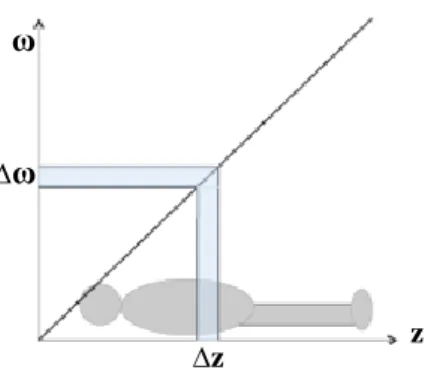
Figure 2.3: The principle of slice selection. By applying a RF pulse with a finite bandwidth (∆ω), only the spins in a slice thickness (∆𝑧) are excited, equation 2.11. Adapted from [34]. ... 10

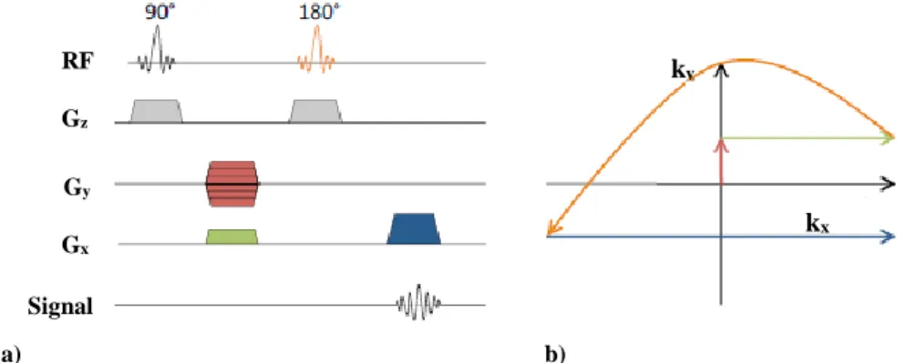
Figure 2.4: SE MR sequence. a) Schematic of a 2D SE sequence. b) K-space trajectory in the 𝑘𝑥 and 𝑘𝑦 plane. The data is acquired, while scanning the blue line in k-space. Adapted from [34]. ... 11

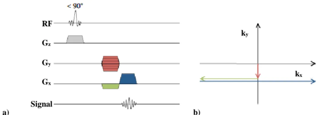
Figure 2.5: GE MR sequence. a) Schematic of a 2D GE sequence. b) K-space trajectory in the the kx and ky plane. Adapted from [33]. ... 12

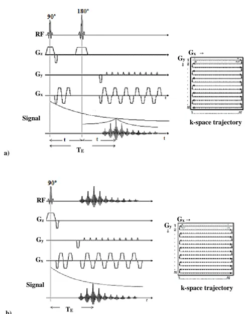
Figure 2.6: 2D EPI sequence and respective k-space trajectory. a) Schematic 2D SE and k-space trajectory. b) Schematic 2D GE and k-space trajectory [40]. ... 13

Figure 2.7: K-space acquisition. a) Single-shot. b) Multi-shot EPI acquisition. Adapted from [42]. ... 14

Figure 2.8: EPIK sequence. a) Schematic representation of the k-space trajectory. Each k-space trajectory is divided into three distinct regions: a keyhole region (kx) and two sparse regions (ks). The solid, dashed and fine-dashed lines in ks regions indicate the sampling positions performed at the 1st, 2nd and 3rd measurements, respectively. b) Brain images acquired in 3T. On the left EPI and on the right EPIK respectively. Adapted from [44]. ... 14

Figure 2.9: The principle of a gradient coil generating a linear gradient in the z-direction. a) Using two coils perpendicular to the z-axis on both sides of the imaging volume, in which opposing currents are induced. b) A linear gradient magnetic field is created in which the field depends on the z-position. Adapted from [34]. ... 16

Figure 2.10: Main features of PET. Adapted from [54]. ... 17

Figure 2.11: PET imaging principle. a) After the annihilation of a positron and an electron, two 511 keV photons are emitted in opposite directions (~180°). b) When two interactions are simultaneously detected within a ring of detectors surrounding the patient, it is assumed that an annihilation occurred on LOR connecting the two interactions. By recording many LORs the activity distribution can be tomographically reconstructed. Adapted from [57]. ... 18

Figure 2.12: PET events. a) Scatter. b) Random coincidences. c) Attenuation. Adapted from [34]. ... 19

Figure 2.13: PET data acquisition. a) 2D. b) 3D. Adapted from [63]. ... 22

Figure 2.14: Features of MR/PET. Adapted from [32]. ... 25 Figure 2.15: Different designs for combined clinical MR/PET systems. a) Patients can be shuttled between

separate MR/PET systems operated in different rooms. b) Patients are positioned on a common table platform between stationary PET and MR systems; the delay between the MR and PET examination is reduced (Philips Healthcare). c) Patients are positioned inside an integrated MR/PET gantry (Siemens

(16)

xiv

Figure 2.16: Hybrid 3T MR-BrainPET system present in INM-4 Forschungszentrum Jülich. The BrainPET

is inserted between the magnet and the MR coils. Adapted from [88]. ... 27

Figure 2.17: BrainPET component. Brain PET insert, detector cassette and detector block respectively.

Adapted from [88]. ... 28

Figure 2.18: Vessel caliber in solid tumors. a) Normal blood vessels. b) Tumor blood vessels. Normal

vessels form highly organized capillary beds, which are well suited for the delivery of O2 and nutrients to

the tissue. The red vessels indicate oxygen-rich feeding arteries and arterioles, blue vessels are veins carrying deoxygenated blood and the intermediate regions indicate a transient capillary stage. Tumor vessels are disorganized with large, tortuous vessels, blind ends and frequent branching, which may lead to poor perfusion and collapse of non-functional vessels. Slow blood flow is indicated by reduced color intensity. The points represent hypoxic regions. Adapted from [95]... 31

Figure 3.1: Perfusion EPI. a) DSC. b) ASL. The plots in the bottom row show data for a typical volume

of interest (VOI), in WM. Adapted from [4]. ... 34

Figure 3.2: CTC curve. ... 35 Figure 3.3: Multi-echo GESE EPI perfusion. a) EPI images in a selected patient acquired during baseline

(top row) and at the peak of the bolus passage (bottom row). b) MRI signal time course of each EPI train in a specified voxel within GM. The dark blue color corresponds to TE1, the green to TE2, the red to TE3

the light blue to TE4 and the purple to TE5. Adapted from [102]. ... 40

Figure 3.4: Cerebrovascular network. Arterial system corresponds to red and venous system to blue.

Adapted from [105]. ... 41

Figure 3.5: Vessel vortex curve from GE SE pairwise relaxation curves. Adapted from [12]. ... 45 Figure 3.6: Relaxation curves and respective direction of the voxel curve. a) ∆R2GE* and ∆R2SE.b)

Clockwise vessel vortex curve. c) ∆R2GE* and ∆R2SE. d) Counter-clockwise vessel vortex curve. On figure

a, SE signal peaks earlier than the GE signal resulting in a counter-clockwise vortex (figure d). On figure c, GE signal peaks earlier than the SE signal resulting in a clockwise vortex (figure b). Adapted from [12]. ... 45

Figure 4.1: CTC. a) Conventional bolus curve. b) Bolus curve fitted using a GVF. In green it is represented

the ∆R2SE curve and in blue the ∆R2SE curve fitted. ... 51

Figure 5.1: The estimated vessel size index (Vsi) in μm in different ROIs (WM, GM and tumor region) for each patient. In blue, it is represented the WM, in orange GM and in gray the tumor. Vsi was calculated for the whole brain by computing both ∆R2GE* and ∆R2SE fitted curves using equation 3.21. ... 56

Figure 5.2: The estimated blood volume (CBV) in mL/100g indifferent ROIs (WM, GM and tumor region) for each patient. In blue it is represented the WM, in orange GM and in gray the tumor. CBV was calculated for the whole brain by computing ∆R2GE* fitted curve using equation 3.9. ... 56

Figure 5.3: The estimated mean vessel density (Q) in s-1/3_{in different ROIs (WM, GM and tumor region)}

for each patient. In blue it is represented the WM, in orange GM and in gray the tumor. Q was calculated for the whole brain by computing both ∆R2GE* and ∆R2SE fitted curves using equation 3.14. ... 57

(17)

xv

List of Tables

Table 5.1: Combination of PW metrics (Vsi, CBV and Q) information in tumor area comparing with the brain tissues of normal-appearing WM. If the vessel caliber, density and blood volume increased, the box is filled with an up arrow. Otherwise with a down arrow. ... 61

Table A.1: Patients information. Patient number, sex and histologic information. Regarding the histologic

information, all the patients had a positive 18F-FET tumor exame HGG: High Grade Glioma, LGG: Low Grade Glioma, A: Astrocytoma, OA: Oligoastrocytoma and GBM: Gliobastoma.. ... 77

Table A.2: The estimated Vsi in different ROIs (WM, GM and tumor region) for each patient. Mean,

standard deviation and the respective difference in normal (WM and GM) and tumor tissue in percentage. The mean and the standard deviation was calculated for all the pixels between the 16 slices. The percentage was calculated using the formula WM,GM (%)= (1−(WM,GM)/Tumor) x 100 ... ... 78

Table A.3: A.3: The estimated CBV in different ROIS (WM, GM and tumor region) for each patient. Mean,

standard deviation and the respective difference in normal (WM and GM) and tumor tissue in percentage. The mean and the standard deviation was calculated for all the pixels between the 16 slices. The percentage was calculated using the formula WM,GM (%)= (1−(WM,GM)/Tumor) x 100 ). ... 79

Table A.4: The estimated Q in different ROIs (WM, GM and tumor region) for each patient. Mean, standard

deviation and the respective difference in normal (WM and GM) and tumor tissue in percentage. The mean and the standard deviation was calculated for all the pixels between the 16 slices. The percentage was calculated using the formula WM,GM (%)= −((1−(WM.GM)/Tumor) x 100).. ... 80

Table A.5: Distance values between the hot spots of 18_{F-FET data with Vsi, CBV and Q. The distance was}

(18)

(19)

xvii

List of Abbreviations

EXPLANATION ABBREVIATION/SYMBOL TE TR ∆R2GE* ∆R2SE 11_C-MET 18_F-FDG 18_F-FET ADC AIF ASL BBB BET CA CBF CBV CT DCE DSC DWI EPI EPIK FAST FID FLAIR FOV FSL FT GD-DTPA GE GM GVF LOR LSO MP-RAGE MR MRI MTT NMR PET PWI Q RF Echo -Time Repetition Time T2* Relaxation Rate T2 Relaxation Rate [11_{C]-Methyl-L-Methionine} [18_{F]-Fluoro-Deoxy-Glucose} O-(2-[18_{F] Fluorethyl)-L-Tyrosine} Apparent-Diffusion-Coefficient Arterial Input Function Arterial Spin Labeling Blood-Brain Barrier Brain Extraction Tool Contrast Agent Cerebral Blood Flow Cerebral Blood Volume Computed Tomography Dynamic Contrast Enhanced Dynamic Susceptibility Contrast Diffusion-Weighted Imaging Echo-Planar Imaging

Echo-Planar Imaging with Keyhole FMRIB's Automated Segmentation Tool Free Induction Decay

Fluid-Attenuation Inversion Recovery Field of View

FMRIB Software Library Fourier Transform

Gadolinium Diethylenetriamine Pentaacetic Acid Gradient-Echo

Gray-Matter

Gamma Variate Function Line of Response Lutetium Oxyorthosilicate

Magnetization Prepared Rapid Gradient-Echo Magnetic Resonance

Magnetic Resonance Imaging Mean Transit Time

Nuclear Magnetic Resonance Positron Emission Tomography Perfusion-Weighted Imaging Mean Vessel Density Radio Frequency

(20)

xviii TBR

TF

Tumor to Brain Ratio Transmitted Fraction TTP TVOI VAI VEGF VSI WHO WM mVD Vsi Time to Peak

Tumor Volume of Interest Vessel Architecture Imaging Vascular Endothelial Growth Factor Vessel Size Imaging

World Health Organization White Matter

Mean Vessel Diameter Vessel Size Index

(21)

1

1.

Context and Outline

1.1 Introduction

Medical imaging is a powerful tool used in modern medicine for disease diagnosis, for localizing tumors and screening treatment response. Magnetic Resonance Imaging (MRI) and

Positron Emission Tomography (PET) have become the most important imaging techniques in

modern radiology. These techniques revealed an important usage in neuro-oncology due to its capability of early tumor detection (e.g. localization, state of growth and activity) [1].

Although its ability to differentiate tumor tissue and to assess tumor heterogeneity information from nonspecific tissue changes is limited. Three-dimensional (3D) contrast-enhanced MR imaging currently remains the method of choice for glioma diagnosis. Therefore, to gain additional functional information on tumor biology (e.g. vasculature), advanced MR imaging techniques, particularly Perfusion Weighted Imaging (PWI), are increasingly used [2]. Currently, Dynamic Susceptibility Contrast (DSC) is the most common method used to measure perfusion in brain tumors [3]. DSC-MRI relies on the intravenous injection of a paramagnetic contrast agent (e.g. Gadolinium-Diethylenetriamine Pentaacetic Acid (Gd-DTPA)) and the rapid measurement of the transient signal changes during the passage of the bolus through the brain [4]. Cerebral Blood Volume (CBV) is one the most relevant parameter derived from DSC-PWI. In brain tumors, CBV shows a significant correlation with microvessel density and its volume is, typically, larger, compared to healthy brain tissues [5, 6].

Besides MRI, radiolabeled amino acids PET have been successfully used in brain tumor diagnosis. Amino acid PET measures the magnitude of amino acid transport and its distribution in the tumor. In the tumor area, the incorporation of the amino acid is increased comparing to healthy tissue and these differences can be imaged [7]. Among the available PET tracers, 18_F-FET

exhibited a better performance in neuro-oncology, proved by an accurate tumor area delineation and glioma grading, when comparing with others available tracers and MRI techniques [8-11].

In the cases of radiation therapy or biopsy, there are some major problems that affect planning: the precise delineation of vital tumor tissue and the missed information about the heterogeneity of the vessels in tumor tissues. Hereupon, the combination of PWI and 18_F-FET

information has been proposed for clinical practice and an accurate delineation and the assessment of complementary information about tumor localization, size, growth and perfusion can be obtained [12,13].

Several studies have been performed by combing PWI and amino acid PET information in gliomas. Despite a good correlation found between CBV and amino acid PET tracers uptake [11-13], a recent study revealed that active tumor tissue of gliomas as depicted by 18_F-FET

information provides a better performance on tumor delineation when compared with CBV measured with PWI [13]. Also, a poor correlation, a poor spatial congruence and different hot spot localization found within both techniques supported this conclusion. Thereby, due to the lack of results from the present parameters derived from PWI (e.g. CBV), in this dissertation, it is proposed an improvement of PWI computation parameters and its comparison with 18_F-FET

information.

For this purpose, the PWI-MR sequence developed in the Forschungszentrum Jüllich was adopted in this work. This sequence acquires multiple contrasts (Gradient and Spin echo (GE and SE)) taking the advantages of the Echo-Planar Imaging with Keyhole (EPIK) acquisition scheme [14]. By combining GE and SE a new PWI methodology emerged, the so-called Vessel Size

(22)

2 of vessels caliber and density and about the distribution of the different types of vessels (arteries, veins and capillaries), which is otherwise not directly accessible using others PW parameters. Moreover, as brain tumors are characterized by abnormal and heterogeneous poorly constructed vasculature, associated to an increased microvessel caliber and decreased density, vascular information shows to be widely important particularly in tumor diagnosis, monitoring and therapy [24].

In this manner, due to the good performance of 18_{F-FET in tumor delineation and the}

vascular information provided by VSI, a metabolic guided vascular analysis can be performed. This vascular analysis could improve the major problems that impact the tumor planning being reliable important in particular for glioma monitoring.

1.2 Outline of the Thesis

The overall aim of the work discussed here was to perform a metabolic guided vascular analysis of brain tumors by combining 18_{F-FET PET information and VSI information obtained}

from MR PWI using multi-echo EPIK sequence. Previous publications have shown an unsatisfactory conformity by the combination of CBV derived from PW and 18_{F-FET information}

for tumor delineation. In this way, the new PW sequence was explored to compute new parameters, named VSI. Thereby, PW parameters and 18_{F-FET information will be combined and}

compared in order to provide metabolic and vascular information, essential for tumor monitoring and treatment planning.

This thesis is organized in six chapters described below. The present Chapter 1 introduces the context, motivation and general organization of the work.

Chapter 2 introduces a comprehensive explanation of the relevant theoretic

underpinnings of this work. This chapter is subdivided into four sections where the MRI, PET and MR/PET modalities and the brain tumors topic are introduced. The first section, describes the MRI basic principles, followed by a description of the imaging principles, MR sequences and instrumentation. The second section describes the strategies for acquiring functional images with PET, from the positron annihilation to the post-correction images. The data acquisition, reconstruction and correction methods, as well as PET instrumentation are explained. The third section describes the multi-modal MR/ PET approach and its application in brain studies. Advantages, design difficulties and instrumentation (BrainPET system) are also described. Finally, in the last section, a brief introduction to brain tumors, particularly regarding gliomas, will be addressed with a focus on its vasculature and diagnosis issues.

Chapter 3 discusses the strategies described in the literature to provide an accurate tumor

diagnosis using PWI-MR and 18_{F-FET PET information. Tumor Vasculature using VSI}

methodology is explored and the main motivation of this work is addressed. Clinical and human studies for VSI methodology, gliomas studies using 18_{F-FET PET and the combination of PWI}

and amino acid PET tracers will be reviewed.

In Chapter 4, materials and methods developed in this dissertation are described. Patients information, MRI and PET acquisitions and processing methodology will be addressed (e.g. co-registration, segmentation, masking and tumor delineation). In addition, the methodology used to fit the Concentration Time Curve (CTC) (Gamma fitting) will be described, as well as the features used to analyze the data.

Chapter 5 presents the results obtained in this work from the methodologies explained in Chapter 3 and 4.

(23)

Chapter 1. Context and Outline

3 Finally, in Chapter 6, a detailed discussion of the entire thesis is presented as well as the conclusion and future perspectives of this work.

(24)

(25)

5

2.

Medical Imaging in Oncology– MR/PET

Basics

In this chapter, the principal theoretical concepts required for the understanding of the main content of the remaining chapters of this dissertation are given. An overview on Medical

Imaging in Oncology will be exploited where Magnetic Resonance Imaging (MRI) and Positron Emission Tomography (PET) will be introduced. Hybrid Imaging technique for application in

brain studies will also be explored. Also a brief introduction about brain tumors and its inherent vasculature, particulary for gliomas, will be performed.

2.1 Introduction

Medical Imaging is a group of different imaging modalities used to obtain images from the body. In clinical practice, medical images are a key tool for diagnostic and treatment purposes. Therefore, medical imaging plays an important role in initiatives to improve public health for all population groups [1]. Nowadays, a wide number of medical imaging techniques are available such as Computed Tomography (CT), PET and MRI [1]. Each technique has strong and weak highlights. Since 1990, the combination of more than one image modality has been introduced, named Hybrid Imaging. The combination of PET with CT and MR with PET are the main hybrid imaging techniques. Both provide further and complementary information compared to their separate purchase. Using hybrid imaging, an accurate diagnosis can be obtained with a special interest in MR/PET for brain tumors diagnosis [25].

2.2 Magnetic Resonance Imaging (MRI)

Nuclear Magnetic Resonance (NMR) has its roots in the pioneering work of Rabi et al.

[26] Bloch et al. [25] and Purcell et al. [28] in the first half of the century XX. In 1944, Rabi who the first to show the effect of radiofrequency (RF) wave with the Larmor Frequency on nuclear magnetic moments. For the discovery of a resonance method for recording the magnetic properties of atomic nuclei, he has received the Nobel Prize in Physics. In 1946, Bloch and Purcell devised virtually identical methods for measuring nuclear magnetic moments. While Purcell discovered the phenomenon of nuclear magnetic resonance in solids (e.g. solid paraffin) [28], Bloch discovered it in liquids (e.g. water) [27]. Since these findings, NMR has been widely used to study the magnetic properties of molecules. The step from NMR to MRI was made by inventions of Lauterbur in 1973 [29]. Both researches showed that it is possible to manipulate the local magnetic fields using gradient fields. Therefore, these findings enabled the introduction of MRI, which has since then been a very successful imaging technique.

MRI is a nuclear medical imaging technique that allows imaging in vivo the human morphology, structure and dynamics with a high contrast and resolution. The main characteristics of MRI are present in the diagram of figure 2.1. MRI is a 3D technique, allowing to imaging multiple body planes without changing the subject position during the acquisition [30, 31]. This technique uses magnetic fields and electromagnetic energy to generate signals from the atomic

(26)

6 nuclei, in particular, the hydrogen nuclei (proton of the nuclei), which can be translated into images. In this subsection, the concepts related to MRI involved in this work will be introduced.

Figure 2.1: Features of MRI. Adapted from [32].

2.2.1 Basic Principles

Magnetic Resonance (MR) technique focuses on the atomic nuclei magnetic properties

in order to provide anatomical images of the human body. In MR, the preferred nucleus is the hydrogen nucleus (1_{H) because it is the most abundant in water (75%) and in the human body.}

Nevertheless, imaging of other nucleus such as sodium (23_{Na) and potassium (}19_{K) is also possible}

[30, 31].

In the absence of an external magnetic field, the protons precess around random directions and orientations. Therefore, they compensate each other and the net value of the magnetization of the whole cohort is null. Otherwise, in the presence of an external homogenous magnetic field (B0), the spinsbecome quantized processing in two orientations. While one state is aligned

parallel (spin-up), the other is aligned anti-parallel (spin-down) to the direction of the magnetic field. The energies of two states are given by:

E = μ. B0= γℏI. B0 with μ = γJ = γℏI (2.1)

,where μ is the magnetic moment, 𝛾 the gyromagnetic ratio, J the angular momentum, ℏ the Planck’s constant divided by 2π, I the spin angular momentum that can be ±1

2 for protons and B0

the external magnetic field [33].

The spin-up (parallel) state has a slightly lower energy than the spin-down (anti-parallel) state. The energy difference between both levels is the energy needed for a proton to swap between the two states that is associated with the electromagnetic frequency required. The energy difference is given by:

0 1 2 3 4 5 Anatomy Function Temporal Resolution Spatial Resolution Development Prospects Technology Maturity Clinical Availability Clinical Utility Sensitivity/Specificity Molecular Imaging

(27)

Chapter 2. Medical Imaging in Oncology: MRI

7 ∆E = γℏ. B0 (2.2)

From the energy equation 2.2 the precessional frequency can be introduced, named

Larmor Frequency (ω0), equation 2.3.

ω0= γB0 (2.3)

This frequency depends on the strength of the external magnetic field B0 and of the

gyromagnetic ratio(γ ). For protons, the Larmor frequency is approximately 42.6MHz in a magnetic field of 1T.

Since the parallel state is slightly favoured, there are more protons in the spin-up than in the spin-down state. The number of protons in each state (Nup|Ndown) follow the Boltzmann’s

distribution in thermal equilibrium, equation 2.4.

Nup

Ndown= e ∆E

kBT_{≈ 1 +}γℏB0

kBT (2.4)

, where kB is the Boltzamann’s constant and T is absolute temperature in degrees Kelvin.

The difference between the number of protons is each state (Nup− Ndown) creates the

Net Magnetization (M0), equation 2.5.

M0= (Nup− Ndown) . μ =

ργ2ℏ2B0

4kBT (2.5)

, with the proton density ρ and μ =1

2γℏ.

While the protons contributing to the net magnetization are all out of phase, the sum, meaning the net magnetization is exactly aligned with the magnetic field B0 and can be measured

[10].

2.2.1.1 RF Pulses

The magnetization is measured in the transverse (xy) plane where a time-varying part of the magnetization induces a signal in the receiver coils. The signal obtained in the coil is the so called Free Induction Decay (FID).

Even though there is a rotating component in this plane, the net magnetization is parallel to B0 with no component in the xy plane. Therefore, the magnetization must be tipped from

equilibrium into it. An alternating magnetic field B1 having the same frequency as the Larmor

frequency to be in resonance with the precessing spins must be applied to achieve this. These pulses are named Radio-Frequency (RF) pulses.

The spins can absorb energy and notate away from the longitudinal axis while precessing around it in the laboratory frame of reference. In a rotational frame of reference, only the nutation would be visible [33].

(28)

8 After the pulse is applied, the spins precess in phase and can therefore be detected. The flip-angle (α) depends only on the amplitude of B1 and duration tp of the RF field and can be

calculated by:

α = γ ∫ B1(t)dt t_p

o (2.6)

2.2.1.2 Relaxation

When the RF pulse stops, the magnetization returns to equilibrium i.e. spins loss the transversal component. This process is called Relaxation and is induced by two independent processes. First, the dephasing of the spins (Spin-Lattice interaction) and second the loss of energy absorbed during the pulse (Spin-Spin interaction) [30].

The spin-lattice interaction results in the recovery of Mz after applying a RF pulse. This

mechanism reflects the time necessary to realign the protons with B0 by transferring protons

energy to surrounding molecules. T1 relaxation is mathematically explained by an exponential

behaviour, equation 2.7. For a 90° RF pulse, T1 relaxation is defined as the time taken for 63% of

M0 to recover after a 90°RF pulse, figure 2.2.

Mz(t) = Mz0(1 − e −t

T1_{) (2.7)}

, where Mz0is the equilibrium magnetization.

Otherwise, spin-spin interaction is the mechanism that results in a decrease of Mxy after

applying a RF pulse. The loss of phase coherency of protons due to the changes on protons mobility causes the reduction of Mxy. Mathematically this process is explained by equation 2.8.

For a 90° flip-angle, T2 relaxation corresponds to the time it takes for 37% of Mxy to be obtained

due to relaxation of transverse magnetization, figure 2.2.

Mxy(t) = Mxy0e −t

T2_(2.8)

, where Mxy0 is the equilibrium magnetization

Furthermore, T2 is also influenced by the inherent field inhomogeneities, resulting in a

faster decay. In this case, the relaxation will occur at a rate of T2*. T2* is shorter than T2 and is

given by: 1 T₂∗ = 1 T2+ 1 Tinhom= 1 T2+ γ∆B (2.9)

, where 𝛾 is the gyromagnetic ratio and ∆B the relaxation rate contribution attributable to field inhomogeneities across a voxel.

Since these processes take time to occur and the time taken is intrinsic to each tissue, it is possible to establish a correspondence between tissue type and the signal acquired.

(29)

9

Figure 2.2: T1 and T2 relaxation times [33]. Although they happen at the same time, for a certain tissue T2 is much smaller than T1. This fact can not be visible in other tissues because the relation between both curves can be different.

2.2.2 Image Principles

2.2.2.1 Slice Selection

As it shown by equation 2.3, the resonance frequency of a spin is proportional to the field applied. In the presence of the static magnetic field, a RF pulse with the Larmor frequency will excite all spins in the imaging volume. However, it is possible to excite only a specific part of the imaging volume.Changes on the static field have to be done using a linear magnetic gradient [30]. By applying a linear magnetic gradient field in the z-direction (Gz), the amplitude of the

magnetic field will vary with position (z). Consequently, the resonance frequency will also depend on the position:

ω(z) = γ(B0+ zGz) (2.10)

When a RF pulse is transmitted with a specific range of frequencies just the protons with the Larmor frequency that match the RF pulse frequency are excited, the so-called Slice Selection. The principle is depicted in figure 2.3. The thickness of the excited slice depends on the bandwidth (∆ω) of the RF pulse and the steepness of the gradient, equation 2.11 [31].

∆𝐳 =

∆𝛚 𝛄𝐆𝐳

(2.11) Mz Mxy 0.37M0 M0 0.63M0 T1 Recovery T2 Decay Mz

(30)

10

Figure 2.3: The principle of slice selection. By applying a RF pulse with a finite bandwidth (∆ω), only the spins in a

slice thickness (∆𝐳) are excited, equation 2.11. Adapted from [34].

2.2.2.2 Frequency and Phase Encoding

Slice selection method does not differentiate between protons within each slice. Therefore, two additional gradients are usually applied in order to encode the spins in the slice. Those are named Gy and Gx depending on their direction. The first one corresponds to the Phase

Encoding Gradient in the y direction and the second one to the Frequency Encoding Gradient in

x direction respectively. Both gradients have identical properties but are applied in different directions and at different times. Since the three gradients (Gx,Gy, Gz) are applied, the spins can

now be coded in all three directions (x, y and z).

2.2.2.3 K-Space and Image Reconstruction

In MRI, the spatial frequency domain is called K-Space and was introduced in 1983 by Ljunggren [35] and Twieg [36].

The 2D discrete Fourier Transform (FT) of the image yields a function, which describes the distribution of spatial frequencies kxand ky. The space of spatial frequencies is called k-space

and is the inverse space of the physical co-ordinate system (x, y). The spatial frequency variables kxand kyare related to the time on gradient variables. Therefore, k-space data is just the MRI

time domain data with a substitution of variables (t, (Gx,Gy, Gz)) to (kx, ky) [36].

K-space can be filled with information that codifies the image in the frequency domain. Therefore, by applying a FT on the k-space, the image reconstruction can be performed. For 2D imaging, a 2D FT is applied. For 3D images, the procedure is the same as explained for 2D but one more spatial frequency (kz) and coordinate (z) is considered. Also, a 3D FT is applied for 3D

imaging.

2.2.3 Image Sequences

A pulse sequence is simply the definition of RF and gradient pulses, where the time interval between pulses, their amplitude and the shape of the gradient affect the characteristics of the MR image. MRI pulses sequences are widely important allowing the acquisition of images with different kinds of contrast.

z

ω

∆ω

(31)

11 The Repetition Time (TR) and the Echo Time (TE) in milliseconds describe most

sequences. TRis the time from the application of an excitation pulse to the application of the next

pulse. TE refers to the time between the application of RF excitation pulse and the peak of the

signal induced in the coil.

The two main types of MR pulse sequences used are Spin-Echo (SE) and Gradient-Echo (GE) sequences. The remaining developed MR sequences derive in some way from the combination of the SE and GE. Both sequences will be explained bellow.

2.2.3.1 Spin-Echo (SE)

In a SE sequence after the 90° RF excitation pulse, the refocusing of the spins is obtained by applying a 180º RF pulse. After the RF pulse, a Gy gradient fields are applied to spatially

encode the spins and a 180º pulse is applied to rephrase the spins along with the same slice selective gradient. The signal (echo) is then acquired at TE. A schematic overview of a SE

sequence and respective sampled k-space is illustrated in figure 2.4 [33].

As shown in figure 2.4a, the 90º RF excitation pulse is applied together with a slice selection gradient. After the RF excitation, a Gy is applied along the y-axis. The amplitude of this

gradient determines the coordinate ky of the line that will be sampled in k-space (orange line),

figure 2.4b. The 180º RF pulse is then applied together with the same slice selection gradient to flip the spins and make them rotate back towards coherence. The signal is acquired around TE,

while a Gx along the x-axis is switched on. This Gx scans a line in k-space in the kx direction (blue

line). Usually, Gx with the same polarity is applied during the phase-encoding gradient in order

to move the k-vector towards the beginning of the line that is to be acquired (negative kx).

Furthermore, in order to acquire the others k-space lines, the process has to be repeated with a determined TR.

a) b)

Figure 2.4: SE MR sequence. a) Schematic of a 2D SE sequence. b) K-space trajectory in the kx and ky plane. The data is acquired, while scanning the blue line in k-space. Adapted from [34].

2.2.3.2 Gradient- Echo (GE)

As implied by the name, in GE sequence gradients are used to diphase and rephrase the transverse magnetization vector instead of the 180º RF pulse. In GE sequence, an RF pulse is applied partially flipping the net magnetization vector into the transverse plane (flip-angle). A first gradient is applied to diphase and then a gradient with opposite sign is applied to rephase the spins [33]. RF Gz Gy Gx Signal kx ky

(32)

12 GE sequence begins with the application of a RF excitation pulse simultaneously with the slice selection gradient. When the excitation pulse is turned off, the protons begin to dephase and Gy is applied along the y-axis. Simultaneously, a negative Gx is applied along the x direction

in order to induce a faster dephasing of the protons. Thereafter, a positive Gy is applied to rephase

the protons at the same time as the echo is measured (TE), figure 2.5a. As well as SE sequence,

the amplitude of the gradient determines the kx and ky coordinates of the line, which will be

sampled in k-space, figure 2.5b. Here a shorter TR can therefore be achieved when compared to a

SE sequence, leading to shorter total acquisition times.

Furthermore, in GE sequence the refocusing of spins are purely based on gradients and not on a 180° pulse. Thereby, the local field inhomogeneities due to susceptibility effects are not compensated by the echo and the signal is dependent of T2* rather than T2. This leads to T2*

-weighted images instead of T2-weighted images.

a) b)

Figure 2.5: GE MR sequence. a) Schematic of a 2D GE sequence. b) K-space trajectory in the kx and ky plane. Adapted from [33].

2.2.3.3 Echo-planar Imaging (EPI)

Echo-planar Imaging (EPI) was introduced by Sir Peter Mansfield in 1977 who received

the Nobel Prize in 2003 for his contribution to MRI and medical field [37].

EPI is a fast MRI pulse sequence that uses multiple GE with different phase steps in order to sample the k-space. In EPI, multiple lines of the k-space are acquired after a single RF excitation. The rephasing gradient reverses the spatial variation of the phase of transverse magnetization caused by a dephasing gradient. Thereby, the echoes acquisition will be accomplished by rapidly reversing the readout gradient or for a Gx along the x-axis [37].

Like a conventional SE sequence, an SE EPI sequence begins with 90°and 180° RF pulses. However, after a 180° RF pulse a short Gy gradient (blip) is applied promoting a rapid

oscillation of Gx from a positive to a negative amplitude along the x-axis, forming a train of

gradient-echoes. Each echo is phase encoded differently by encoding blips on the phase-encoding axis. Further, each Gx oscillation corresponds to one line of imaging data in k-space and

each blip results on a transition from one line to the next. In GE EPI sequences, the image is acquired after a single RF excitation pulse and uses the gradient to generate the echoes following the same process explained before. A schematic representation of a 2D SE and GE EPI sequence is illustrated in figure 2.6. ky kx ky RF Gz Gy Gx Signal kx ky

(33)

Chapter 2. Medical Imaging in Oncology: MRI 13 a) b)

Figure 2.6: 2D EPI sequence and respective k-space trajectory. a) Schematic 2D SE and k-space trajectory. b)

Schematic 2D GE and k-space trajectory [40].

2.2.3.3.1 Single-Shot and Multi-Shot EPI

Regarding the k-space sampling, EPI sequences can be divided into two groups:

Single-Shot and Multi-Single-Shot or also named segmented. The main difference between both sequences is on

the k-space acquisition.

In a single-shot sequence, in a single excitation (one shot) the entire range of phase encoding steps are acquired [41]. Therefore, all of the k-space data are acquired in only one shot, achieved by generating and reading all of the required echoes from a single FID, figure 2.7a. However, the image acquisition matrix is typically no larger than 128x128. Nowadays, single-shot EPI is the most widely available fast imaging sequence on clinical scanners and facilitates whole-brain coverage at reasonable Signal to Noise Ratio (SNR)1_{. Single-shot can easily be}

1_{SNR measures the signal strength relative to background noise.}

Gx Gy RF Gz Gy Gx Signal k-space trajectory Gy Gx TE Signal RF Gz Gy Gx k-space trajectory Gx Gy TE

(34)

14 applicable because does not need specialized gradient amplifiers to perform the required gradient switching.

In multi-shot sequence, more excitations are needed to acquire the information of one slice. Also, the range of phase steps is equally divided into several "shots" per slice. Thereby, a subset of Gx is acquired within each TRand the k-space is acquired in each shot. The shots are

repeated until a full set of data is collected, figure 2.7b. This sequence can be applied in Diffusion -Weighted Imaging (DWI) and PWI due to the shorter TE [41].

Comparisons between single-shot and multi-shot EPI reported that in multi-shot, the SNR is higher than in single-shot due to the shorter TE and presents less susceptibility artifacts due to

shorter readouts. However, this sequence requires longer TR when compared to single-shot for the

same number of slices and resolution [41].

a) b)

Figure 2.7: K-space acquisition. a) Single-shot. b) Multi-shot EPI acquisition. Adapted from [42].

2.2.3.4 Echo-planar Imaging with Keyhole (EPIK)

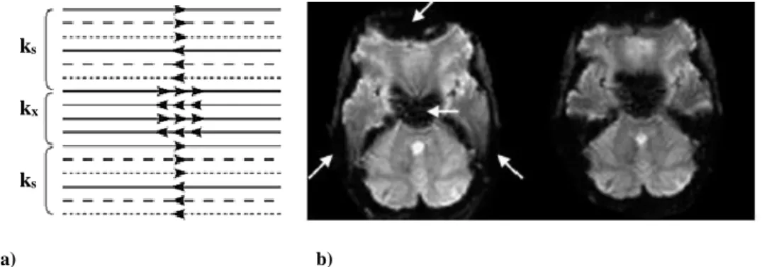
An alternative to EPI sequence is named Echo-planar Imaging with Keyhole (EPIK) proposed by Shah et al. [43] and validated by Zaitsev et al. at 1.5T [14]. In EPIK, in the acquisition, each measurement scans the central k-space region completely, whilst the peripheral space regions are sparsely sampled resembling a multi-shot scheme, figure 2.8a. A complete k-space can be reconstructed by sharing the sparse region data from the consecutive scans. By applying EPIK sequence, improvements in temporal resolution, reduced signal-loss and reduced image artifacts compared to the single-shot EPI are achieved, figure 2.8b [14, 43].

a) b)

Figure 2.8: EPIK sequence. a) Schematic representation of the k-space trajectory. Each k-space trajectory is divided

into three distinct regions: a keyhole region (kx) and two sparse regions (ks). The solid, dashed and fine-dashed lines in ks regions indicate the sampling positions performed at the 1st, 2nd and 3rd measurements, respectively. b) Brain images acquired in 3T. On the left EPI and on the right EPIK respectively. Adapted from [44].

ks

(35)

15

2.2.4 Instrumentation

While MRI instruments vary considerably in design and specifications, all MRI scanners include several essential components. The Main Magnetic Field, Gradient Field Magnets and RF

Coils are the three principal components.

First, for the subject to be scanned a main magnetic field is required. This magnetic field is generally constant in time and space, provided by a variety of magnets. The purpose of these magnets is to induce a net nuclear spin magnetization to the volume of interest.

Second, to induce spatial changes in the polarized magnetic field, gradient field magnets with a specific time and spatial dependencies are required. These spatial changes are able to manipulate the net nuclear spin magnetization so that it is dependent on the spatial localization in the volume.

Lastly, RF coils, both transmitter and receiver coils, are respectively required to transmit RF waves to the volume and to detect the resulting MR signal. While the transmitter coil creates the external B1 field necessary to excite the nuclear spin, the receiver coil detects the weak signal

emitted by the spins as they precess in the B0 field [45].

2.2.4.1 B

0

Field

In MRI, the B0 field strength can vary from 0.1T to 14.7T. For clinical practice, the

systems currently in use have a field strength of 3T or lower, most commonly 1.5T. In the most systems, a superconducting magnet, using a superconductor current loop, generates a B0 field.

Niobium-tin and niobium-titanium cooled with liquid helium are the superconductors commonly used. Beyond superconducting magnet, resistive magnets can also be used. In spite of requiring more power and operate at lower field strength (≈0.2T), they can be used in so-called open-magnet MRI systems, whose are better tolerated by claustrophobic patients [45]. In research, higher field strengths are used, which can only be generated by superconductor magnets. For human whole-body imaging 7T [46] and for brain imaging up to 9.4T magnets are available [47].

2.2.4.2 Gradient Coils

Gradient coils are used for position encoding. Three pairs of gradient coils are used enabling the generation of linear magnetic gradient fields in the x, y and z directions. A magnetic gradient field is created by placing two coils perpendicular to the axis in which the gradient needs to be created, on both sides of the imaging volume. By inducing currents with opposing directions in the coils, both coils will induce opposite magnetic fields along the axis. As the strength of the field created by a coil depends on the distance from the loop, the sum of the fields from both coils is a linear gradient [46]. The principle of a gradient coil is illustrated in figure 2.9.

(36)

16

a) b)

Figure 2.9: The principle of a gradient coil generating a linear gradient in the z-direction. a) Using two coils

perpendicular to the z-axis on both sides of the imaging volume, in which opposing currents are induced. b) A linear gradient magnetic field is created in which the field depends on the z-position. Adapted from [34].

2.2.4.3 RF Volume Resonator

RF Volume Resonators are cylindrical or multi-loop coils, which generate a B1field

perpendicular to the bore axis. RF volume resonators are able to excite the MR signal, essential when deep tissue has to be measured or if a coil does not provide convenient patient access [45]. A typical design of RF volume resonator in both clinical and animal MR scanner is named birdcage resonator [48]. Commonly used as a head or body coil, birdcage resonators can be used in both transmit-receive and only transmit configurations. This coil is used to achieve homogeneous excitation over a subject. The multi-channel coil configuration is advantageous because speeds up the acquisition. Surface coils can also be used to excite the MR signal. Nonetheless, as they can only detect signals from a superficial region, are not so useful for clinical practice.

Z

Bz BZ1

(37)

17

2.3 Positron Emission Tomography

In 1957, Anger invented the gamma camera considered the start of modern nuclear medicine imaging. Since this invention, some design and operation modifications were done (e.g. pinhole collimators2_{and a rotating gamma camera) allowing tomographic images reconstruction}

and afterword’s, single photon emission images computation [49]. Following a different track than single-photon imaging, in 1959 Anger and Rosenthal presented the first gamma camera with positron-imaging capability [50]. Positron imaging was used at first place to image 52_Fe

radiotracer distributed in the bone marrow of patients with hematological diseases3_{[51]. Some}

years later, in 1964, Robertson and Bozzo [52] introduced the first design that resembles the currently used scanner. However, as at that time the computer systems were not powerful enough to enable this system integration, only more than one decade later and after several modifications the device was used for brain imaging [53]. Since the early 1980’s, PET was introduced and used in many major hospitals.

PET is a powerful nuclear medicine imaging technique that can be used to measure metabolic activity or body function processes in vivo. The main features of PET are presented in the diagram of figure 2.10. In clinical practice, the patient receives a small intravenous injection of a radiotracer that follows the same pathways as the biomolecules of the body [53]. Therefore, PET images the kinetics and distribution of these biomolecules by detecting the radioactive decay. The concepts related to PET involved in this work will be introduced.

Figure 2.10: Main features of PET. Adapted from [54].

2.3.1 Basic Principles

To measure the physiological and biochemical process of a single molecule in vivo, this technique uses the tracer principle, which states that a radioactive material participates in

2_{Pinhole collimators have a single hole that drilled into the sheet with high atomic number material.} 3_{Related to blood disorder.}

0 1 2 3 4 5 Anatomy Function Temporal Resolution Spatial Resolution Development Prospects Technology Maturity Clinical Availability Clinical Utility Sensitivity/Specificity Molecular Imaging