An Evaluation of the Accuracy of Models for the
Determination of the Weighted Mean
Temperature of the Atmosphere
V. B. Mendes1, G. Prates2, L. Santos3, and R. B. Langley41Laboratório de Tectonofísica e Tectónica Experimental (LATTEX), Faculdade de Ciências da Universidade de Lisboa (FCUL), Portugal; 2Escola Superior de Tecnologia da Universidade do Algarve, Portugal; 3FCUL, Portugal; 4Geodetic Research Laboratory, Department of Geodesy and Geomatics Engineering, University of New Brunswick, Canada.
BIOGRAPHIES
Virgílio Mendes is an assistant professor in the Faculty of Sciences of the University of Lisbon, Portugal. He has a Diploma in Geographic Engineering from the University of Lisbon and a Ph.D. in Surveying Engineering from the University of New Brunswick. His principal areas of research are the modeling of tropospheric delay in radiometric techniques and the application of the Global Positioning System to the monitoring of crustal deformation.
Gonçalo Prates is an assistant at the University of Algarve, Portugal. He has a Diploma in Geographic Engineering from the University of Lisbon. He is involved in the study of GPS with application to meteorology and vehicle location.
Luis Santos received his Diploma in Geographic Engineering from the University of Lisbon in 1997. In 1998-1999, he was an assistant at that university. He is involved in the application of GPS to Geodesy.
Richard Langley is a professor in the Department of Geodesy and Geomatics Engineering at the University of New Brunswick, where he has been teaching and conducting research since 1981. He has a B.Sc. in applied physics from the University of Waterloo and a Ph.D. in experimental space science from York University, Toronto. Dr. Langley is a co-author of the Guide to GPS Positioning and is a contributing editor and columnist for GPS World magazine.
ABSTRACT
The estimates of the zenith wet delay resulting from the analysis of data from space techniques, such as GPS and VLBI, have a strong potential in climate modeling and weather forecast applications. In order to be useful to meteorology, these estimates have to be converted to precipitable water vapor, a process that requires the knowledge of the weighted mean temperature of the atmosphere, which varies both in space and time.
In recent years, several models have been proposed to predict this quantity. Using a database of mean
temperature values obtained by ray-tracing radiosonde profiles of more than 100 stations covering the globe, and about 2.5 year’s worth of data, we have analyzed several of these models. Based on data from the European region, we have concluded that the models provide identical levels of precision, but different levels of accuracy. Our results indicate that regionally-optimized models do not provide superior performance compared to the global models.
INTRODUCTION
The water vapor content of the atmosphere is the most important variable in establishing the earth’s climate and its short-term changes are an essential piece of information for severe weather forecasting and operational weather prediction [Kuo et al., 1993; Bevis et al., 1994]. Since the late 1940s, the highly variable spatial and temporal distribution of atmospheric water vapor has been essentially determined using a network of stations launching radiosondes. These weather balloons are generally launched throughout the world twice a day and provide height profiles of pressure, temperature, and relative humidity. The major drawbacks of radiosondes are the poor spatial and temporal resolution, and the degradation of the measurements of relative humidity at high altitude, as a result of contamination of the sensors during the flight [WMO, 1987; WMO, 1996].
The water vapor in the electrically neutral atmosphere is responsible for part of the propagation delay of radio signals used by radiometric space geodetic techniques, such as the Global Positioning System (GPS), and very long baseline interferometry (VLBI). The contribution of water vapor to the neutral-atmosphere propagation delay can be converted to precipitable water. Due to its low-cost, high spatial distribution, and continuous measurements, the GPS receiver is an attractive remote sensing tool and can be used to complement the existing radiosonde network in atmospheric research [Rocken et al., 1995; Coster et al., 1996; Ware et al., 1997; Elgered et al., 1997; Emardson et al., 1998].
PHYSICS OF GPS METEOROLOGY
The neutral-atmosphere propagation delay, dna, is given by
(
)
∫
+ − = − ray 6 na 10 Nds L G d , (1)where N = N(s) is the refractivity along the curved ray path (ray), L is the electromagnetic path length and G is the corresponding straight-line path or geometric path. In this equation, the first term on the right-hand side is the excess path delay due to the delay experienced by the signal, and the term in parenthesis is the delay due to the bending of the ray, the geometric delay.
The refractivity of a parcel of air is expressed as [Thayer, 1974]: Z T e K T e K Z T P K N 1 w 2 3 2 1 d d 1 − − + + = , (2)
where Ki are constants empirically determined in laboratory, Pd is the partial pressure due to dry gases, e is the water vapor pressure, T is the temperature, and Zd and Zw are the compressibility factors for dry air and water vapor, respectively [Owens, 1967]. Equation (2) is alternatively written as 1 w 2 3 2 d 1 Z T e K T e K R K N − + + ρ = ' , (3) where − = w d 1 2 2 R R K K K' , (4)
Rd is the specific gas constant for dry air, Rw is the specific gas constant for water vapor, and ρ is the density of moist air (see Mendes and Langley [1999] for details). The first term in Equation (3) is the hydrostatic component of refractivity, whose integration along the zenith direction constitutes the zenith hydrostatic delay,
z h d :
∫
ρ = − a r s r d 1 6 z h 10 K R dz d , (5)where rs is the geocentric radius of the receiver antenna, ra is the geocentric radius of the top of the neutral atmosphere, and dz has length units. The zenith hydrostatic delay can be predicted with good accuracy provided good surface pressure measurements are available [Mendes and Langley, 1999].
The second term in Equation (3) is the wet component of refractivity. Likewise, its integration along the zenith direction constitutes the zenith wet delay, d :zw
dz Z T e K T e K 10 d -w1 a r s r 2 3 2 6 z w
∫
+ = − ' . (6)The zenith wet delay is highly variable and difficult to predict. Therefore, in high-precision applications of space geodetic techniques, the zenith wet delay is typically estimated as a nuisance parameter in the adjustment process.
The elevation dependence of the neutral-atmosphere propagation delay is modeled using a mapping function (see Mendes [1999] for details).
If we introduce the water-vapor-weighted mean temperature of the atmosphere (hereafter mean temperature), defined as [Davis et al., 1985]
∫
∫
= a r s r 1 -w 2 a r s r 1 -w m dz Z T e dz Z T e T , (7)Equation (6) can be written as
dz Z T e T K ' K 10 d 1 w a r s r m 3 2 6 z w − −
∫
+ = . (8)Using the equation of state for water vapor
w w 1 w R Z T e ρ = − , (9)
where ρw is the density of water vapor, we finally get
dz T K ' K R 10 d a r s r w m 3 2 w 6 z w
∫
ρ + = − . (10)The integral in Equation (10) is the integrated water vapor (IWV), defined as the total mass of water vapor in a column of air with cross section of 1 m2 extending from the surface to the top of the atmosphere, usually given in units of kg m-2: dz IWV a r s r w
∫
ρ = . (11)This quantity can be easily converted to length units by dividing by the density of liquid water ( HO 103kgm 3
2
−
≈
ρ ) and be interpreted as the height of an equivalent column of liquid water that would result if the water vapor were condensed, that is, the integrated precipitable water vapor or simply precipitable water (PW) (see Dutton [1986]; Peixoto and Oort [1992 ]):
dz 1 PW a r s r w O H2
∫
ρ ρ = . (12)Substituting Equation (11) into Equation (10), we obtain: IWV
dzw =ξ , (13)
where ξ is a “constant” of proportionality given by:
+ = ξ − m 3 2 w 6 T K ' K R 10 . (14)
The mean temperature is the only unknown in Equation (14) and its estimation plays an important role in the conversion from zenith wet delay to precipitable water from space radiometric measurements. Due to its dependence on the water vapor profile, Tm it therefore variable in space and time. There are different alternatives for estimating Tm, which include the use of: a) a climatological database for the site [Ross and Rosenfeld, 1997; 1999]; b) ray tracing of radiosonde data; c) numerical weather prediction model; d) empirical model based on regression analysis. This paper concentrates on the accuracy analysis of seven empirical models against ray tracing through radiosonde data.
As PW and d have units of length, we can also definezw the following dimensionless quantity:
PW d Q z w = . (15) MODEL DESCRIPTION
The mean temperature model by Bevis et al. [1992] is based on the analysis of ~9,000 radiosonde profiles from sites in the United States, with a latitude range of 27° N to 65° N and a height range of 0 to 1.6 km, for a period of two years (model MB):
s m 70.2 0.72T
T = + , (16)
where Ts is the surface temperature, in kelvins.
Mendes [1999] used 50 sites, covering a latitude range of 62° S to 83° N and a height range of 0 to 2.2 km, with a total of ~32,500 radiosonde profiles for the year 1992. Based on his regression analysis, a revised set of coefficients for Equation (16) was proposed (model UNB98Tm1):
s m 50.4 0.789T
T = + . (17)
Mendes also found that for high latitudes the mean temperature was better modeled using the following relation (model UNB98Tm2):
3 s 6 m 196.05 3.402 10 T
T = + × − . (18)
The models for Q presented by Emardson and Derks [1998] are based on ~129,000 profiles from 38 sites in Europe, with a latitude range of 36° N to 79° N. Two of the suggested models are driven by surface temperature only, as in the previous models. The authors have derived sets of coefficients for the whole region and tailored sets for different climatological areas. In our comparison study, only the regional coefficients have been tested. The simpler model (ED1) assumes a linear relation between Tm and Ts: ∆ + + = T a a a Q 2 1 0
,
(19)where T∆ =Ts−Ts, and T is the mean surfaces temperature for the region (T = 283.49 K). The seconds model (ED2) is the result of a Taylor series expansion as a power series of T∆: 2 2 1 0 aT a T a Q= + ∆ + ∆
.
(20)The third model (ED3) is independent of the surface temperature and is driven by latitude and day of year:
π + π + ϕ + = 365 t 2 cos a 365 t 2 sin a a a Q D 3 D 2 1 0 , (21)
where ϕ is the site latitude in degrees, and tD is the decimal day of year.
Finally, the fourth model (ED4) is a hybrid model which adds a dependence on day of year to ED2, resulting in:
π + π + + + = ∆ ∆ 365 t 2 cos a 365 t 2 sin a T a T a a Q D 4 D 3 2 2 1 0 .(22)
The coefficients for the different ED models are presented in Table 1.
Table 1 − Coefficients for the different ED models.
Coef. ED1 ED2 ED3 ED4
a0 -1.3328980×10⁴ 6.458 5.882 6.457 a1 1.0033568×10¹⁰ -1.78×10⁻² 0.01113 -1.78×10⁻² a2 7.5239894×10⁵ -2.2×10⁻⁵ 0.064 -1.9×10⁻⁵ a3 − − 0.127 1.3×10⁻² a4 − − − -0.4×10⁻² DATA ANALYSIS
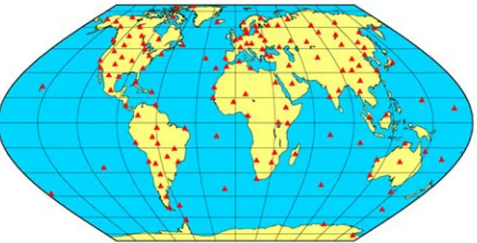
The assessment of the models was performed using ray tracing through radiosonde data from 138 stations, globally distributed (Figure 1). The radiosonde data covers the period 1997.0 to 1999.5, for most of the sites,
with a variable number of balloon launches per day (some sites have 4 launches a day; the norm is 2). The radiosonde data consists of height profiles of pressure, temperature and dew-point. The quality of the data was controlled through a set of procedures, such as: elimination of soundings with no surface data recorded; elimination of levels within a sounding without observations of pressure, temperature and dew-point (except for layers above 10 km, where only pressure and temperature were checked); elimination of levels leading to unreasonable temperature gradients; elimination of soundings with surface temperature or mean temperature exceeding the monthly 95% confidence interval for the site; assurance of a minimum of 8 levels per sounding with the last level beyond the 300 hPa limit.
As most of the radiosonde profiles have reported heights only for mandatory levels, whereas much higher resolution is given for the meteorological variables, the heights for all levels were calculated from reported temperature and pressure using the hypsometric equation [Wallace and Hobbs, 1977; Dutton, 1986]. The agreement between the computed and the reported heights was better than a few tens of metres, at all pressure levels, in the worst cases. Nevertheless, we have found that there were no significant changes in the ray-traced mean temperature values using our computed heights. A total of 152,032 benchmark values were created, with a maximum number for Herstmonceaux, UK (~3500 soundings) and a minimum number for Fortaleza, Brazil (~100 soundings).
Figure 1 − Radiosonde sites location. (Figure produced using the Generic Mapping Tools software [Wessel and Smith, 1995].)
MODEL ASSESSMENT AND DISCUSSION
In order to directly compare the performance of all models, we had to derive expressions for Tm from the
different Emardson and Derks (ED) models. In this process, the refractivity constants of Thayer [1974] were used. As these models were tailored for Europe, we limit the discussion on the performance of the models to this geographic region only (19 stations with a total of 29,460 traces). The performance for the other geographic regions will be discussed elsewhere.
The ED3 model performs poorly for all stations, confirming that the use of surface temperature is essential in obtaining a higher accuracy in PW determination. The ratio between the standard deviations of ED3 and ED4 varies between 1.3 (station 8508, Lajes, Azores) and 4.6 (station 33345, Kiev, Ukraine) with a mean value of 2.9 ± 0.8. The other 3 ED models perform very similarly both in mean bias and rms scatter (about the mean value), as shown in Figure 2.
For this group of stations, the improvement in rms scatter of ED4 with respect to ED1 is below 0.1 K and there are two stations where ED1 performs better than ED4 (also by a very small margin). The mean value of these differences is 0.05 K ± 0.04 K. As regards the mean bias, ED1 has in general a slight positive bias (0.05 K ± 0.04 K).
The differences in rms scatter between ED2 and ED4 vary between 0.02 K and 0.1 K, with a mean value of 0.06 K± 0.02 K; that is, for this group of stations ED2 performs systematically worse than ED4. The model is nevertheless less biased than ED1, with a mean difference of 0.03 K ± 0.03 K with respect to ED4.
From this analysis we can conclude that, with the exception of ED3, all the ED models perform similarly, as the differences obtained in both the mean bias and rms scatter can not be considered significant.
Figure 2 − Differences in performance between the ED1, ED2 and ED4 models (stations ordered by increasing latitude; station number according to the World Meteorological Organization).
The other models tested were developed using no (MB) or little (UNB98Tm1 and UNBTm2) data from Europe. For this reason, these models are slightly biased in comparison to ray-traced values for European sites. However they
Differences in rms scatter 85 08 85 79 171 30 170 62 154 20 74 81 348 58 110 35 108 68 333 45 38 82 62 60 268 50 61 81 264 22 25 27 29 63 12 41 40 18 Mo d e l mi n u s R e fe r e n c e ( K ) -0.2 -0.1 0.0 0.1 0.2 ED1-ED4 ED2-ED4
Differences in mean bias
8 508 8 579 1 7130 1 7062 1 5420 7481 3 4858 1 1035 1 0868 3 3345 3882 6260 2 6850 6181 2 6422 2527 2963 1241 4018 Mo d e l m in u s R e f e re n c e ( K ) -0.2 -0.1 0.0 0.1 0.2 ED1-ED4 ED2-ED4
show similar levels of precision. In fact, for a few of the 19 European stations, all these models perform better than ED4. The basic statistics are presented in Table 2. These results show that there is little gain in tuning the models for a particular region, as regards the mean bias, and almost no gain in reducing the rms scatter.
Table 2 − Statistics for the differences in mean bias and rms scatter (numbers in parenthesis) between MB, UNB98Tm1, UNB98Tm2 and ED4.
MB Minus ED4 UNB98Tm1 minus ED4 UNB98Tm2 minus ED4 Mean 0.99 (0.06) 0.69 (0.06) 0.36 (0.09) Rms scatter 0.21 (0.06) 0.14 (0.05) 0.24 (0.08) Minimum 0.51 (-0.04) 0.40 (-0.04) 0.02 (-0.03) Maximum 1.25 (0.18) 0.86 (0.16) 0.89 (0.22)
The performance of the different models with respect to our ray traces is shown in Figure 3. For the total number of differences between the different models and ray tracing, the box-and-whisker plots represent the following statistical quantities: median and mean (thinner and thicker lines inside the boxes, respectively), 25th and 75th percentiles (vertical box limits), 10th and 90th percentiles (whiskers), and 5th and 95th percentiles (open circles).
It can be concluded that all models have a small positive bias and similar levels of precision (excluding ED3). The mean bias for UNB98Tm1 (1 K) is slightly larger than the one obtained for UNB98Tm2 (0.7 K), showing that the relation with a cubic dependence on the surface temperature is efficient in modeling the mean temperature. These two models are less biased than MB (mean bias of 1.3 K). As regards the rms scatter about the mean value,
all models perform essentially identically (between 3.02 K, for ED4, and 3.10 K, for UNB98Tm2); ED1, ED2 and UNB98Tm1 have the same rms scatter (3.07 K) and MB has an rms scatter of 3.08 K. The rms scatter for the total number of residual differences allows us to conclude that the mean temperature can be computed with a relative precision of ~1.1 % (at the one-sigma level), considering an average mean temperature of ~270 K representative of a European atmosphere. This precision is slightly worse for other geographic areas.
ACKNOWLEDMENTS
Radiosonde data was provided by the British Atmospheric Data Center (BADC). The ray-trace software was developed by James Davis, Thomas Herring, and Arthur Niell. We thank Ragne Emardson and Henricos Derks for making their models available prior to publication.
REFERENCES
Bevis, M., S. Businger, S. Chiswell, T.A. Herring, R.A. Anthes, C. Rocken, and R.H. Ware (1994). “GPS meteorology: Mapping zenith wet delays onto precipitable water.” Journal of Applied Meteorology, Vol. 33, No. 3, pp. 379-386.
Bevis, M., S. Businger, T.A. Herring, C. Rocken, R.A. Anthes, and R.H. Ware (1992). “GPS meteorology: Remote sensing of atmospheric water vapor using the Global Positioning System.” Journal of Geophysical Research, Vol. 97, No. D14, pp. 15,787-15,801. Coster, A.J., A.E. Niell, F.S. Solheim, V.B. Mendes, P.C.
Toor, K.P. Buchmann, and C.A. Upham (1996). “Measurements of precipitable water vapor by GPS, radiosondes, and a microwave water vapor radiometer.” Proceedings of ION GPS-96, the 9th International Technical Meeting of the Satellite Division of The Institute of Navigation, Kansas City, Mo., 17-20 September, pp. 625-634.
Davis, J.L., T.A. Herring, I.I. Shapiro, A.E.E. Rogers, and G. Elgered (1985). “Geodesy by radio interferometry: Effects of atmospheric modeling errors on estimates of baseline length.” Radio Science, Vol. 20, No. 6, pp. 1593-1607.
Dutton, J.A. (1986). The Ceaseless Wind: An Introduction to the Theory of Atmospheric Motion. Dover Publications, New York.
Elgered, G., J.M. Johansson, B. Rönnäng, and J.L. Davis (1997). “Measuring regional atmospheric water vapor using the Swedish permanent GPS network.” Geophysical Research Letters, Vol. 24, No. 21, pp. 2663-2666.
Emardson, T.R. and H.J.P. Derks (1998). “On the relation between the wet delay and the integrated precipitable water vapour in the European atmosphere.” Submitted to Meteorological Applications.
Figure 3 − Box-and-whisker plot for the differences between the different models and ray tracing, for the European region. (Note: VM1 = UNB98Tm1, VM2 = UNB98Tm2). MB ED 1 ED 2 ED 4 VM 1 VM 2 Mo d e l m in u s Tra ce ( K ) -8 -6 -4 -2 0 2 4 6 8
Emardson, T.R., G. Elgered, and J.M. Johansson (1998). “Three months of continuous monitoring of atmospheric water vapor with a network of Global Positioning System receivers.” Journal of Geophysical Research, Vol. 103, No. D2, pp. 1807-1820.
Kuo, Y.-H., Y.-R. Guo, and E.R. Westwater (1993). “Assimilation of precipitable water measurements into a mesoscale numerical model.” Monthly Weather Review, Vol. 121, No. 4, pp. 1215-1238.
Mendes, V.B. (1999) Modeling the Neutral-atmosphere Propagation Delay in Radiometric Space Techniques. Ph.D. dissertation, Department of Geodesy and Geomatics Engineering Technical Report No. 199, University of New Brunswick, Fredericton, New Brunswick, Canada.
Mendes, V.B. and R.B. Langley (1999). “Tropospheric zenith delay prediction accuracy for high-precision GPS positioning and navigation.” Navigation, Vol. 46, No.1, pp. 25-34.
Owens, J.C. (1967). “Optical refractive index of air: Dependence on pressure, temperature and composition.” Applied Optics, Vol. 6, No. 1, pp. 51-59.
Peixoto, J.P. and A.H. Oort (1992). Physics of Climate. American Institute of Physics, New York.
Rocken, C., T. van Hove, J. Johnson, F. Solheim, R. Ware, M. Bevis, S. Chiswell, and S. Businger (1995). “GPS/STORM – GPS sensing of atmospheric water vapor for meteorology.” Journal of Atmospheric and Oceanic Technology, Vol. 12, pp. 468-478.
Ross, R.J. and S. Rosenfeld (1997). “Estimating mean weighted temperature of the atmosphere for Global Positioning System applications.” Journal of Geophysical Research, Vol. 102, No. D18, pp. 21,719-21,730.
Ross, R.J. and S. Rosenfeld (1999). “Correction to “Estimating mean weighted temperature of the atmosphere for Global Positioning System applications.”” Journal of Geophysical Research, Vol. 104, No. D22, p. 27,625.
Thayer, G.D. (1974). “An improved equation for the radio refractive index of air.” Radio Science, Vol. 9, No. 10, pp. 803-807.
Wallace, J.M. and P.V. Hobbs (1977). Atmospheric Science: An Introductory Survey. Academic Press, New York.
Ware, R., C. Alber, C. Rocken, and F. Solheim (1997). “Sensing integrated water vapor along GPS ray paths.” Geophysical Research Letters, Vol. 24, No. 4, pp. 417-420.
Wessel, P. and W.H. Smith (1995). “New version of the generic mapping tools.” EOS Transactions of the AGU, Vol. 76, p. 329.
World Meteorological Organization (WMO) (1987). “WMO international radiosonde comparison (UK, 1984, USA, 1985): Final report (J. Nash and F.J. Schmidlin).” Instruments and Observing Methods Report No. 30, WMO/TD-No. 195, Geneva.
World Meteorological Organization (WMO) (1996). “WMO international radiosonde comparison - Phase IV: Final report (S. Yagi, A. Mita, and N. Inoue).” Instruments and Observing Methods Report No. 59, WMO/TD-No. 742, Geneva.