A Recursive Construction of the Regular
Exceptional Graphs with Least Eigenvalue
−
2
I. Barbedo, D. M. Cardoso, D. Cvetkovi´
c, P. Rama, S.K. Simi´
c
∗Abstract.
In spectral graph theory a graph with least eigenvalue−2 is exceptional if it is con-nected, has least eigenvalue greater than or equal to−2, and it is not a generalized line graph. A (κ, τ)-regular setSof a graph is a vertex subset, inducing aκ-regular subgraph such that every vertex not inShasτneighbors inS. We present a recursive construction of all regular exceptional graphs as successive extensions by regular sets.
Mathematics Subject Classification (2010). Primary 05C50; Secondary 06A06. Keywords. Spectral graph theory, exceptional graphs, posets.
1. Introduction
LetG= (V(G), E(G)) be a simple graph, whereV(G) denotes the nonempty set of vertices and E(G) the set of edges. It is assumed that G is of order n, i.e. |V(G)| = n. An edge of E(G), which has the vertices i and j as end-vertices is denoted by ij. When there is an edge between the vertices i and j we say that these vertices are adjacent. The neighborhood of a vertex u ∈ V(G), NG(u), is the set of vertices adjacent tou, that is, NG(u) ={v ∈V(G) :uv∈E(G)}. The degree of vertexu is the cardinality of its neighborhood. A graphG isr-regular (or regular of degreer) if each vertex of Ghas the same degree r.
Throughout the paper, AG denotes the adjacency matrix of G, that is AG = (aij)n×n, where aij = 1 if ij ∈E(G) andaij = 0 otherwise. The eigenvalues of the graph G are the eigenvalues of its adjacency matrix, here ordered such that
λ1 ≥λ2 ≥ · · · ≥λn. A detailed treatment of graph eigenvalues can be found in [8].
∗The authors I. Barbedo, D. M. Cardoso and P. Rama were partially supported by Portuguese
A pair (X,B) is a 1−(v, l, λ) design, if X is a set with cardinality v and B is a family ofb subsets of X with cardinality l, called blocks, and each element
x∈X lies in exactly λblocks. The incidence matrixB of a 1−(v, l, λ) design is thev×bmatrix withij-entry equal to 1 ifxi∈Bj and 0 otherwise. Alternatively, a 1−(v, l, λ) design (X,B) can be represented by a semi-regular bipartite graph with parameters (v, b, λ, l), i.e. by a bipartite graph withvvertices of degreeλin one colour class, andb vertices of degreel in another colour class.
A connected graph with least eigenvalue greater than or equal to−2 is either a generalized line graph (with line graphs included), or an exceptional graph (see, e.g., [11]). According to [11, Proposition 1.1.9], a regular connected generalized line graph (see definition, e.g., in [11, Section 1.1]) is either a line graph or a cocktail party graph (a regular graph on 2k vertices of degree 2k−2). A graph is said to beexceptionalif it is connected, has least eigenvalue greater than or equal to−2, and it is not a generalized line graph. It is known [10] that an exceptional graph has at most 36 vertices, with vertex degrees at most 28. There are exactly 187 regular exceptional graphs. They are divided into three subsets (to be defined later) called layers. These graphs are constructed in [11, 1, 2] using different techniques. A comprehensive survey of problems on graphs with least eigenvalue at least−2, including exceptional graphs, can be found in [11].
A vertex subset S ⊆V(G) of the graphG is a stable (or independent) set if no pair of vertices in S is connected by an edge. A stable set with maximum cardinality is a maximum stable set.
Given a graph G, a partition π = (V1, . . . , Vr) of the vertex set of G is an
equitable partition, if for any pairi, j∈ {1, . . . , r} there existsdij ∈N0 such that
for allv∈Vi dij=|NG(v)∩Vj|, that is, the number of neighbors that a vertex of
Vi has inVj is independent of the choice of the vertex in Vi.
A (κ, τ)-regular setSof a graphGis a vertex subset which induces aκ-regular subgraph such that every vertex not in S hasτ neighbors inS. If Gis a regular graph, then a (κ, τ)-regular setS defines an equitable bipartition inG.
The (κ, τ)-regular sets appeared first in [16], under the designation of eigen-graphs, and also in [15], in both cases in the context of strongly regular graphs and designs. Later on, the (κ, τ)-regular sets were investigated in the general context of arbitrary graphs [4, 6, 5].
The aim of this paper is to present a recursive construction of all regular ex-ceptional graphs based on the new (κ, τ)-extension technique suggested in [3]. It recursively generates the families of regular exceptional graphs along with a partial order relation among them, and this is represented by its Hasse diagram.
In Section 2 we describe the (κ, τ)-extension technique of a regular graphG
by a regular graphH, and also the partial order relation that arises. The process of extending a graph is reduced to the construction of the incidence matrices of a 1-design (or an appropriate bipartite semi-regular graph).
of the 1-design desired, stating some proprieties. In addition, we also propose an algorithm to construct the regular exceptional graphs in each layer.
In Section 4 we describe, in more details, the computational results that were obtained by the algorithm for the three layers.
The Appendix contains for each regular exceptional graph the list of other reg-ular exceptional graphs with a minimal number of vertices in which it is contained as a proper induced subgraph.
2. Construction of regular graphs by (κ, τ
)-extensions
LetGbe a (p−τ)-regular graph of ordern1(withτ >0) andH aκ-regular graph (withκ < p) of ordern2. Our aim is to obtain ap-regular graphH⊕G, of order
n2+n1, such that each vertex inGhasτ neighbors inH, and each vertex inH has exactly p−κneighbors inG(hence V(H) is a (κ, τ)-regular set in H⊕G). The procedure that generates the graphH⊕GfromGis called a (κ, τ)-extension ofG of sizen2. This construction is possible if we can define a family,S, ofn1subsets in V(H), calledblocks, each of them with cardinality τ, so that each v ∈ V(H) is in exactlyp−kblocks of S, that is, (V(H),S) is a 1−(n2, τ, p−k) design. Note that there is a 1−(n2, τ, p−k) design if and only if n1
n2 = p−κ
τ . Hence the adjacency matrix ofH⊕Gis given by
AH B
BT A G
,
where AH and AG are the adjacency matrices of H and G, respectively, and B is the incidence matrix of a 1−(n2, τ, p−κ) design, that is, each column of B
is the characteristic vector of a block. Further on, we shall use graph theoretical terminology and consider the corresponding semi-regular bipartite graphs.
The (κ, τ)-extension of a regular graph G by a regular graph H to obtain another regular graphH ⊕G, can be applied recursively to generate a sequence of regular graphs. Considering the (p−τ)-regular graph G and the κ-regular graph H described above, starting with G0 = G, we can generate a set F of ((p−τ) +mτ)-regular graphs,Gm, of ordern1+m n2, where eachGmis obtained by a (κ, τ)-extension ofGm−1 (m≥1). Consequently, we can define the following
partial order relationonF, or on any set of graphs.
Definition 2.1. Given κ, τ, s, if G, G′
are regular graphs, then G G′
if and only ifG′
can be obtained fromGby a sequence of zero or more (κ, τ)-extensions of sizes.
3. Construction of regular exceptional graphs
layer, if the following holds, respectively:
(i) n= 2(r+ 2)≤28,
(ii) n= 3
2(r+ 2)≤27 andGis an induced subgraph of the Schl¨afli graph,
(iii) n= 4
3(r+ 2)≤16 andGis an induced subgraph of the Clebsch graph.
There are 163 graphs in the 1st layer, 21 in the 2nd layer and 3 in the 3rd layer, i.e. 187 in total.
The regular exceptional graphs are completely described in Table A3 in [11, pp. 213-227]. As in [11], regular exceptional graphs are denoted by numbers 1−187.
Let L be the set of regular graphs whose least eigenvalue is greater than or equal to -2. Hence L includes all regular exceptional graphs. We shall consider subsetsL1, L2, L3 of L in which the ratio r+2n (n the number of vertices, r the
degree) is the same as in layers 1, 2, 3, respectively. Hence, each layer is a subset of the corresponding setL1,L2 orL3.
Let Gbe a regular graph of degree r and ordern. Let α(G) be the size of a maximum stable (or independent) set ofGandλn its least eigenvalue. Then
α(G)≤ −nλn
r−λn
.
This inequality is known as the Hoffman inequality although A.J. Hoffman never published it. For some bibliographical details related to this bound see [3].
In [3] it is noted that in the case of regular exceptional graphs of the 1st and 2nd layers, the Hoffman upper bound is attained and is equal to the cardinality of a maximum stable set, which is 4 and 3, respectively. This observation has an empirical character and is based on an inspection of the regular exceptional graphs. In fact, the Hoffman bound is attained for a regular graph Gif and only ifG
has a (0, τ)-regular set such that τ =−λn. The necessary condition was proved in [14] (see also [13, Lemma 9.6.2]) and the sufficient condition was proved in [7]. The following theorem stems from [12].
Theorem 3.1. LetGbe anr-regular graph andλn=−τ its least eigenvalue. For
any stable setS of sizes and characteristic vectorz, we have:
s≤ nτ
r+τ.
Furthermore, the following are equivalent: (i) Equality holds.
(ii) zis a linear combination of ar-eigenvector and aλn-eigenvector.
(iii) The bipartite subgraph induced by the partition {S, V(G)\S} is semi-regular.
It is easy to prove that the stability number of regular exceptional graphs from the first layer is 3 or 4, in the 2nd layer is 2 or 3, and in the 3rd layer is 2. In fact, ifS is a maximum stable set of anr-regular graphG, then
n−α(G) =
[
i∈S
NG(i)
≤X
i∈S
|NG(i)|=α(G)r⇒α(G)≥
n r+ 1.
Therefore, taking in account the relation between the ordern of the regular ex-ceptional graphs and their regularities in each layer, combining the Hoffman upper bound with the above lower bound, the result follows.
However, in spite of some efforts, we were not able to prove theoretically that the Hoffman upper bound is attained in regular exceptional graphs in the 1st and 2nd layer.
We shall construct all regular exceptional graphs from the first and second layer by (0,2)-extensions. For the first layer the (0,2)-extension will have size 4 and for the second layer the size is 3. Applications of (0,2)-extensions will create a stable set of the corresponding size in the resulting graph. This stable set will be a maximum stable set by the Hoffman bound and, from this construction, we may conclude that the Hoffman upper bound is attained for all regular exceptional graphs in the 1st and 2nd layer.
The graphs from the 3rd layer will be considered separately and they will be built by (1,3)-extensions.
With each type of (κ, τ)-extension we consider the corresponding partial order relation.
As observed in [3], we may state the following result.
Theorem 3.2. Regular exceptional graphs are not minimal elements of the posets
(L1,)and(L2,).
As we shall see the same holds for (L3,).
Together with L1, L2, L3 one can study the posets E1, E2, E3 of exceptional
graphs from the three layers with corresponding relations. It would be interesting to study the structure of all these posets. The setsL1, L2, L3 are infinite while
the setsE1,E2,E3 contains 163, 21, 3 elements respectively.
Throughout the recursive construction, starting from a regular exceptional graphG1, with least eigenvalue−2, every regular graphGi, with i≥2, obtained by (κ, τ)-extensions and with least eigenvalue−2, remains an exceptional graph.
This conclusion is a consequence of the fact that the graph property of being a line graph is a hereditary property. This means that any induced subgraph of a line graph is also a line graph. Hence we have the following proposition.
Proposition 3.3. Let Gbe a regular graph with least eigenvalue−2. Let H be a regular induced subgraph ofG. We have
(i) if Gis a line graph thenH is also a line graph,
3.1. Construction of regular exceptional graphs in the 1st layer by (0,
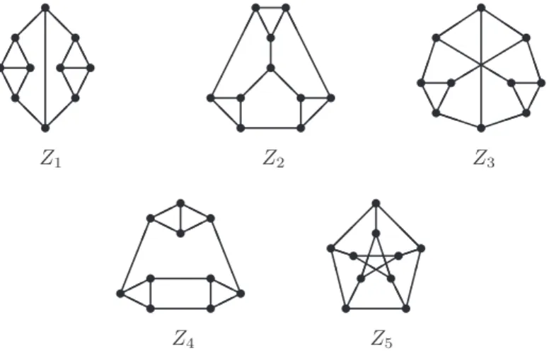
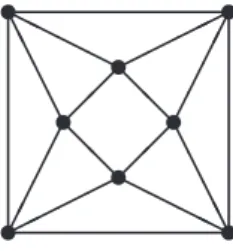
2)-extensions of size 4. The smallest regular exceptional graphs in the first layer are the five graphsZ1,Z2,Z3,Z4andZ5of order 10 and degree 3, given in Figure 1 (taken from [11, Appendix A.3]).
s s
s s
s s
s s s s
❅ ❅ ❅❅ ❆ ❆ ✁✁ ✁ ✁ ❆❆ ❆ ❆ ✁✁ ✁ ✁ ❆❆ Z1 s s s s s s s s s s ❅ ❅ ✁✁ ✁✁✁ ❆ ❆ ❆ ❆ ❆ ❅❅ ❆ ❆ ✁✁ Z2 s s
s s s s
s s
s s
P P P ✏✏✏
✑ ✑ ✑ ◗◗◗ ❆ ❆ ✁✁ ❆ ✁✁❆ ✂ ✂✂ ❜ ❜ ❜❜ ❇❇❇ ✧ ✧ ✧ ✧ Z3 s s s s s s s s s s ❍❍ ✟✟ ✟ ✟❍ ❍ ☞☞ ☞☞ ▲ ▲ ▲ ▲ ✟✟ ❍ ❍✟ ✟ ❍❍ Z4 s s s s s s s s s s ❈ ❈ ❈ ✄✄ ✄ ❅ ❅❅ ✂ ✂✂❇❇❇ P P ❜❜✧✧✏✏ ✁✁ ❆❆ Z5
Figure 1. The smallest regular exceptional graphs in the 1st layer.
These graphs are obtained by (0,2)-extensions of the graph 3K2of order 6 and regularity 1, which is a line graph.
The 8 exceptional graphs of order 12 and regularity 4, are obtained by (0, 2)-extensions of graphs of order 8 and regularity 2, that is, one of the three graphs 2C4,C3∪˙C5(disjoint union of graphsC3andC5) orC8, which are also line graphs.
Since for regular exceptional graphs of the first layer r = n
2 −2, with 10 ≤ n≤28, in order to build the Hasse diagram of the first layer partially ordered by the relation, this set of exceptional graphs is divided into two partially ordered subsets: the graphs with even regularity, obtained by (0,2)-extensions from a graph with even regularity, and the graphs with odd regularity, obtained by (0, 2)-extensions from a graph with odd regularity.
IfGis a graph of even ordernand regularityr= n
2−2 andH is the 0-regular
graph of order 4, the adjacency matrix of the graph G′ of order n′ = 4 +n and
regularityr′ =4+n
2 −2 =
n
2 obtained from a graphGby a (0,2)-extension is given
by
AG′ =
O4 B
BT A G
,
Assuming as a known fact that in the case of regular exceptional graphs of the 1st and 2nd layers, the Hoffman upper bound is attained all these graphs can be constructed by extending graphs with additional 4 or 3 vertices in the way implied by the above considerations.
Let us describe (0,2)-extensions of size 4 in some detail.
The graphGis extended by 4 vertices which form a set S=V(H). Let 1, 2, 3, 4 be the vertices ofS. Each vertex ofGshould become adjacent to exactly two vertices ofS. Let us define anr-regular multigraphM(S) having the setS as the vertex set. If a vertexv of G becomes adjacent to vertices x, y of S, then there is an edge labelled v between x and y in M(S). In this way, the vertices of G
subdivide the edges ofM(S). There are six 2-element subsets ofS. Constructing
G′ from G by an (0,2)-extension means, in fact, to partition the vertex set of G
into six subsets which, in turn, should be assigned to 2-element subsets of S in such a way thatM(S) is regular of degreer. However, the resulting graphG′need
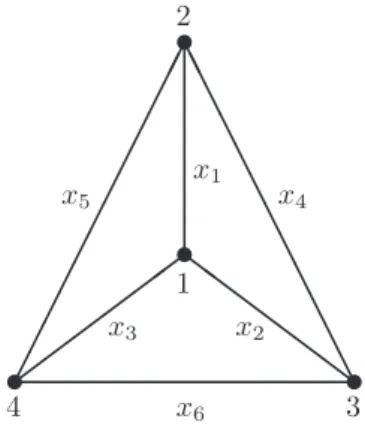
not to be anL-graph, and this should be checked in the actual constructions. A multigraphM(S) can be associated with a weighted complete graph on the four vertices ofS (see Fig. 2). The weightxi on the i-th edge of the multigraph
M(S) represents the number of vertices ofGadjacent to corresponding vertices in
S.
t t
t t
✚✚ ✚✚
✚✚
✁✁ ✁✁
✁✁ ✁✁
✁✁ ✁✁
❩ ❩ ❩ ❩ ❩ ❩
❆ ❆ ❆ ❆ ❆ ❆ ❆ ❆ ❆ ❆ ❆ ❆
1 2
4 3
x1
x6 x5
x2 x3
x4
Figure 2. A weighted complete graph with vertex set{1,2,3,4}.
We have x1+x2+x3 = n/2 since this is the degree of 1 in M(S). Hence,
x4+x5+x6=n/2. We can conclude that the sum of weights of the edges of any star K1,3 and of any triangle K3 is equal to n/2. In addition, we have x1 =x6, x2=x5 andx3=x4.
Now we shall propose an algorithm to construct the 163 graphs of the first layer by (0,2)-extensions which produce equitable partitions.
For a givennconstruct all feasible triplets (x1, x2, x3). For each triplet (x1, x2, x3) we find in turn all ordered partitions of the vertex set ofGinto parts of cardinalities
x1, x2, . . . , x6. For each such partition we consider all graphs Gand extend them to a graphG′ according to this partition. Then, for every graphG′ we calculate
the least eigenvalue and if it is equal to−2 we have generated a regular exceptional graph on n+ 4 vertices. Finally, we should eliminate isomorphic duplicates but record all graph pairs which are in relation.
A suitable computer program based on the above procedure has generated all 163 regular exceptional graph in the first layer. The results are given in the Appendix where for each graph the list of its immediate successors in the posetL is given.
3.2. Construction of regular exceptional graphs in the 2nd layer by (0,2)-extensions of size 3. Using the procedure of construction by (κ, τ )-extensions described in Section 2, our aim is now to build a set of regular graphs obtained by a (0,2)-extension, H⊕G, such thatG is a r-regular graph of order
n, withr= 2n
3 −2, andH is the 0-regular graph of order|V(H)|= 3. Therefore,
this set includes the regular exceptional graphs of the 2nd layer.
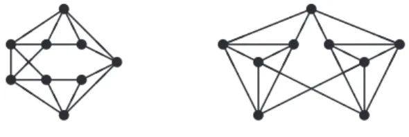
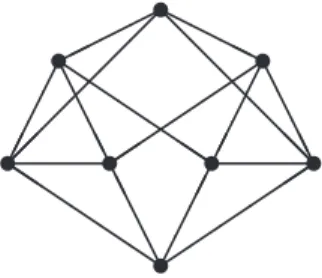
The regular exceptional graphs of the 2nd layer of the lowest order are the graphs of order 9 and regularity 4 in Fig. 3. These graphs are obtained by a (0, 2)-extension of the 2-regular graphC6 and the disconnected graph 2K3, which are line graphs. To construct the Hasse diagram that represents the partially ordered set E2 with relation of the regular exceptional graphs in the second layer, we
consider ther-regular graphs of ordern, withr= 2n
3 −2 and 6≤n≤27.
t t t t t t t t t ◗ ◗ ◗ ❆ ❆ ✁✁ ✑ ✑ ✑ ✁✁❆❅❆❅ ❅ ❅ ❅ ✟✟❍❍ t t t t t t t t t ❆ ❆ ❆ ❆ ✁✁ ✁✁ ✟✟✟✟ ✟✟ ✁✁ ✁✁ ❆ ❆ ❆ ❆ ❍ ❍ ❍ ❍ ❍ ❍ ✦ ✦ ✦ ✦ ✦ ✁✁❛❛❆❆ ❛❛❛ ❍ ❍ ✟✟ ❍ ✟✟❍
Figure 3. The smallest regular exceptional graphs in the 2nd layer.
In fact, in order to construct each adjacency matrix of the graph G′, obtained
fromGby a (0,2)-extension,G′ =H⊕G, it is necessary to determine the incidence
matrix with 3 rows andncolumns.
t C6 t 2K3 t 164 t 165 t 166 t 170 t 167 t 169 t 168 t 174 t 176 t
172 t173 t
171 t
175
t
179 t180 t177 t178
t182 t181
t183 t184 ❩ ❩ ❩ ❩ ✚✚ ✚✚ ❩ ❩ ❩ ❩ ✚✚ ✚✚ ▲ ▲ ▲ ▲ ▲ ☞☞ ☞☞ ☞ ▲ ▲ ▲ ▲ ▲ ✱✱ ✱✱ ✱✱ ❧ ❧ ❧ ❧ ❧ ❧ ❧ ❧ ❧ ❧ ❧ ❧ ▲ ▲ ▲ ▲ ▲ ☞☞ ☞☞ ☞ ✱✱ ✱✱ ✱✱ ▲ ▲ ▲ ▲ ▲ ❧ ❧ ❧ ❧ ❧ ❧ ▲ ▲ ▲ ▲ ▲ ☞☞ ☞☞ ☞ ✁✁ ✁✁ ✑✑ ✑✑ ✑✑ ✁✁ ✁✁ ✑✑ ✑✑ ✑✑ ◗ ◗ ◗ ◗ ◗ ◗ ✁✁ ✁✁ ✑✑ ✑✑ ✑✑ ❆ ❆ ❆ ❆ ❆ ❆ ❆ ❆ ✑ ✑ ✑ ✑ ✑ ✑ ✁ ✁ ✁ ✁ ❛❛ ❛❛ ❛❛ ❛❛ ❛❛ ✁ ✁ ✁ ✁ ❆ ❆ ❆ ❆
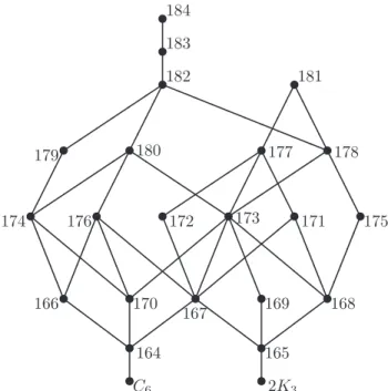
Figure 4. Hasse diagram of graphs from the 2nd layer.
3.3. Construction of regular exceptional graphs in the 3rd layer by (1,3)-extensions of size 4. The exceptional graphs from the 3rd layer are only three. The Hoffman bound is not attained for these graphs. However, it is also possible to build them using the procedure of construction by (κ, τ)-extensions described in Section 2, in this case, by (1,3)-extensions of size 4.
So, the aim now is to build a set of regular graphs obtained by an (1, 3)-extension, H⊕G, such that Gis a r-regular graph of order n, withr = 4n
3 −2,
andH is the 1-regular graph of order 4,i.e. 2K2.
Starting from the line graph 2K2 and extending the graphs in turn by four vertex (1,3)-regular sets we obtained the exceptional graphs 185, 186 and 187. They have 8, 12 and 16 vertices respectively. Graph 185 is presented in Fig. 5. Graph 187 is the well known Clebsh graph.
4. Computational results
Our algorithm was implemented in Matlab R2009b in order to construct the ad-jacency matrices of the regular exceptional graphs of the first layer. Similar algo-rithms were implemented in the cases of the graphs of the second and third layers. The results produced in each layer are described in the Appendix.
t t t t t t t t ✟ ✟ ✟ ✟ ❍❍❍❍ ❍ ❍ ❍ ❍ ✟✟✟✟ ✁ ✁ ✁ ✁ ❆ ❆ ❆ ❆ ❆ ❆ ❆ ❆ ✁✁ ✁✁ ❅ ❅ ❅ ❅
Figure 5. The smallest regular exceptional graph in the 3rd layer.
has four components. Two of these components are associated with the first layer of the regular exceptional graphs: one for the graphs with even degree and the other for the graphs with odd degree.
Notice that there are 3 regular exceptional graphs from the first layer that are not obtained by a (0,2)-extension of the minimal graphs 3K2, 2C4, C3∪˙C5, C8: the 5-regular exceptional graph 17, which is obtained by a (0,2)-extension from the disconnected line graph L1 (see Fig. 6), the 6-regular exceptional graph 56, which is obtained by (0,2)-extension from the 4-regular line graph L2 (see Fig. 6) and the 8-regular exceptional graph 134, which is obtained by (0,2)-extension from the 6-regular line graphL3(see the root graph of L3in Fig. 7)
t
t
t t
t
t t t
t t ❅ ❅ ❅ ❅ ❅ ❅ ❅ ❅ L1 t t t t t t t t t t t t ✁✁ ✁✁ ❆ ❆ ❆❆ ❅ ❅ ❅ ❅ ✁✁ ✁✁ ❅ ❅ ❆ ❆ ❆❆ L2
Figure 6. The line graphsL1 andL2.
The maximal elements in the first layer are the eight regular exceptional graphs of order 20 (113-117, 119-121), all the regular exceptional graphs with order 22 (135-152), and the three Chang graphs (strongly regular exceptional graphs of order 28).
The third component of the Hasse diagram is associated with the regular ex-ceptional graphs from the second layer (see Fig. 4). The minimal elements are
C6 and 2K3 and the maximal elements are the regular exceptional graphs 181 and 184 (the Schl¨afli graph).
t t
t t t t
t t
◗ ◗ ◗ ◗ ◗ ◗
✑✑ ✑✑
✑✑
❆ ❆ ❆ ❆
✁✁ ✁✁ ✁
✁ ✁ ✁
❆ ❆
❆❆ ◗
◗ ◗
◗ ◗◗
✁ ✁ ✁ ✁
❆ ❆
❆❆ ✑ ✑ ✑ ✑ ✑ ✑
❅ ❅
❅ ❅
❅❅ ✟
✟ ✟
✟ ❍❍❍❍
Figure 7. The root graph of the line graphL3.
5. References
References
[1] F.C. Bussemaker, D. Cvetkovi´c, and J.J. Seidel, Graphs related to exceptional root systems. T.H.-Report 76-WSK-05, Technological University Eindhoven, 1976. [2] F.C. Bussemaker, D. Cvetkovi´c, and J.J. Seidel, Graphs related to exceptional
root systems. In Combinatorics, Proc. V Hungarian Colloquium on Combinatorics, Keszthelly 1976 (ed. A. Hajnal, V. T. S´os), Vol. I, Amsterdam-Oxford-New York 1978, 185-191.
[3] D. M. Cardoso and D. Cvetkovi´c, Graphs with least eigenvalue -2 attaining a convex quadratic upper bound for stability number, Bull. Acad. Serbe Sci. Arts, Cl. Sci. Math. Natur., Sci. Math.133(31) (2006), 41–55.
[4] D. M. Cardoso and P. Rama, Equitable bipartitions of graphs and related results,J. Mathematical Sciences120(1) (2004), 869–880.
[5] D. M. Cardoso and P. Rama, Spectral results on graphs with regularity constraints,
Linear Algebra Appl.423(1) (2007), 90–98.
[6] D. M. Cardoso and P. Rama, Spectral results on regular graphs with (κ, τ)-regular sets,Discrete Math.307(11-12) (2007), 1306–1316.
[7] D. M. Cardoso, M. Kaminski, and V. Lozin, Maximumk-regular induced subgraphs,
J. Comb. Optim.14(4) (2007), 455–463.
[8] D. Cvetkovi´c, M. Doob, and H. Sachs,Spectra of Graphs - Theory and Application. Academic Press, New York, 1980.
[9] D. Cvetkovi´c, P. Rowlinson, and S. Simi´c, Graphs with least eigenvalue -2: The star complement technique,J. Algebraic Combinatorics 14(1) (2001), 5–16.
[10] D. Cvetkovi´c, M. Lepovi´c, P. Rowlinson, and S. Simi´c, The maximal exceptional graphs,J. Combinatorial Theory Ser. B,86(2) (2002), 347–363.
[11] D. Cvetkovi´c, P. Rowlinson, and S. Simi´c,Spectral Generalizations of Line Graphs, on Graphs with Least Eigenvalue -2. Cambridge University Press, Cambridge, 2004. [12] C.D. Godsil and M.W. Newman, Eigenvalue bounds for independent sets,
[13] C. D. Godsil and G. Royle, Algebraic Graph Theory. Graduate texts in mathematics. Springer-Verlag, New York, 2001.
[14] W. Haemers, Interlacing eigenvalues and graphs, Linear Algebra Appl. 226/228 (1995), 593–616.
F.C. Bussemaker, D. Cvetkovi´c, and J.J. Seidel, Graphs related to exceptional root systems. In Combinatorics, Proc. V Hungarian Colloquium on Combinatorics, Keszthelly 1976 (ed. A. Hajnal, V. T. S´os), Vol. I, Amsterdam-Oxford-New York 1978, 185-191.
[15] A. Neumaier, Regular sets and quasi-symmetric 2-designs. InCombinatorial Theory
(ed. D. Jungnickel and K. Vedder), Lecture Notes in Mathematics, Vol. 969, Springer, Berlin - Heidelberg 1982, 258–275.
APPENDIX: Extensions of regular exceptional graphs
The data on the 187 regular exceptional graphs are given in Table A3 from the book [11]. These graphs are denoted here by numbers 1 – 187 and these numbers refer to [11]. The graphs are divided into three layers and into smaller groups according to the number of verticesnand the degree r. For each graph the list of regular exceptional graphs obtained by (κ, τ)-extensions is given.
First layer
n= 10, r= 3
1. 14, 16, 18, 22, 23, 24, 27, 28, 30, 32, 33 2. 19, 20, 21, 22, 23, 25, 26, 27, 28, 31, 32, 33, 34 3. 18, 27, 28, 29, 30, 32, 33, 34
4. 15, 16, 18, 19, 20, 24, 25, 26, 27, 28, 29, 30, 31, 32, 33, 34 5. 30
n= 12, r= 4
6. 37, 49, 51, 57, 58, 68
7. 39, 40, 41, 42, 46, 47, 48, 51, 52, 53, 55, 57, 58 8. 39, 40, 42, 55, 57, 61, 63, 64, 65, 66, 67, 68 9. 35, 37, 44, 45, 59, 60, 69
10. 35, 36, 40, 41, 42, 47, 48, 49, 53, 60, 62, 64, 65
11. 35, 37, 38, 39, 40, 46, 47, 48, 49, 50, 51, 54, 59, 60, 62, 63, 64, 67, 68 12. 39, 40, 46, 47, 48, 49, 50, 51, 52, 54, 57, 58, 61, 62, 63, 64
13. 43, 44, 45, 46, 49, 51, 59, 60, 67
n= 14, r= 5
14. 70, 83, 84, 88, 89, 97, 98, 99, 100 15. 81, 82, 90, 95, 96, 105
16. 84, 85, 91, 92, 93, 94, 97, 107 17. 89, 100
18. 90, 92, 94, 97, 99, 101, 103
19. 71, 72, 73, 74, 77, 78, 86, 87, 88, 90, 91, 94, 95 20. 71, 72, 74, 78, 79, 86, 88, 89, 91, 92, 93, 94 21. 78, 88, 93
22. 71, 72, 74, 75, 76, 80, 96, 97, 99, 100, 103, 104 23. 71, 74, 76, 77, 78, 79, 97, 98, 99, 101, 102, 104 24. 71, 72, 75, 76, 81, 84, 91, 92, 94, 100 103, 104 25. 72, 73, 77, 84, 87, 88, 89, 97, 98, 99
26. 71, 77, 78, 82, 83, 86, 91, 97, 102, 104
27. 71, 72, 77, 78, 79, 82, 84, 85, 90, 93, 94, 95, 96, 97, 101, 102, 103 28. 71, 72, 74, 75, 76, 78, 79, 83, 84, 86, 88, 92, 93, 96, 97, 102, 103 29. 86, 90, 94, 106, 107
31. 77, 78, 82, 86, 87, 93, 97, 101, 102, 107
32. 71, 72, 77, 79, 82, 85, 90, 91, 92, 93, 96, 97, 101, 102, 103, 105, 107 33. 71, 72, 75, 76, 78, 79, 83, 84, 86, 88, 89, 91, 94, 97, 98, 99, 100, 102, 103, 104, 106, 107
34. 74, 78, 84, 91, 94, 95, 99, 102, 103, 107
n= 16, r= 6
35. 108, 109, 111, 123, 124, 126, 128, 129, 132 36. 108, 121, 128, 131
37. 110, 111, 112, 123, 124, 129, 130, 133 38. 120, 124, 128
39. 115, 117, 118, 119, 120, 121, 122, 123, 124, 126, 130, 131 40. 116, 117, 119, 121, 123, 124, 125, 126, 127, 128, 129, 133 41. 113, 116, 121, 123, 126, 127
42. 114, 116, 117, 120, 121, 125, 128, 131, 132 43. 108, 109, 122, 130
44. 109, 112, 127, 129 45. 109, 111, 124, 132, 133
46. 113, 114, 115, 116, 118, 119, 122, 124, 126, 127, 128 47. 113, 116, 117, 120, 121, 124, 126, 128, 131
48. 114, 117, 120, 121, 128
49. 113, 116, 119, 123, 124, 127, 129, 133 50. 113, 114, 124, 127, 129
51. 114, 115, 116, 118, 123, 124, 127, 129, 130 52. 118, 119, 121, 122, 125
53. 116, 117, 121, 125, 131 54. 114, 118, 120, 125, 131 55. 114, 116, 117, 120 56. 118
57. 116, 117, 118
58. 113, 114, 115, 116, 117, 118, 119 59. 109, 112, 124, 129, 130, 133 60. 108, 111, 126, 127, 128, 132, 133 61. 114, 117, 118, 119
62. 113, 114, 117, 119, 120 63. 115, 116, 118, 119 64. 116, 117, 120 65. 128
66. 131
67. 127, 130, 132 68. 129
69. 111, 112
70. 142, 143, 146
71. 136, 138, 139, 140, 141, 142 72. 136, 138, 140, 143, 144 73. 135, 136, 142, 145 74. 138, 139, 144, 145 75. 136, 142, 146, 147 76. 136, 138, 143, 147 77. 137, 138, 139, 141 78. 139, 141, 142, 143 79. 138, 141, 144 80. 136, 146 81. 136, 140, 149 82. 137, 140, 141, 152 83. 138, 142, 144, 147, 151
84. 138, 139, 140, 141, 142, 143, 144, 145, 150, 151 85. 140, 141, 152
86. 138, 149, 151 87. 139, 150 88. 142, 150, 151 89. 143, 151
90. 137, 140, 148, 149, 150, 152 91. 141, 144, 149, 151, 152 92. 140, 149, 151
93. 141, 149, 150
94. 140, 145, 149, 150, 151, 152 95. 140, 150, 152
96. 136, 141
97. 138, 139, 140, 141, 142, 143 98. 138, 142
99. 142, 143, 144, 145 100. 143, 144, 146, 147 101. 137, 141
102. 138, 139, 141 103. 140, 141, 144 104. 138, 141, 147 105. 149, 152 106. 151
107. 150, 151, 152
n= 20, r= 8
108. 155, 156, 157 109. 155, 158 110. 153, 159
112. 158, 159 113. 114. 115. 116. 117. -118. 155, 156 119. 120. 121.
-122. 154, 155, 156 123. 153, 155, 156 124. 155, 157, 158 125. 155
126. 156, 158 127. 155, 158 128. 155, 156, 157 129. 153, 158, 159 130. 153, 157, 158 131. 156
132. 155, 157, 160 133. 157, 158, 159 134. 158
n= 22, r= 9
135. 136. 137. 138. 139. 140. 141. 142. 143. 144. 145. 146. 147. 148. 149. 150. 151. 152.
-n= 24, r= 10
153. 161 154. 162 155. 163 156. 162, 163 157. 163 158. 161, 163 159. 161 160. 163
n= 28, r= 12
161. 162. 163.
-Second layer
n= 9, r= 4
165. 167, 168, 169
n= 12, r= 6
166. 174, 176
167. 171, 172, 173, 176 168. 171, 173, 175 169. 173
170. 173, 174, 176
n= 15, r= 8
171. 177 172. 177
173. 177, 178, 180 174. 179, 180 175. 178 176. 180
n= 18, r= 10
177. 181 178. 181,182 179. 182 180. 182
n= 21, r= 12
181. -182. 183
n= 24, r= 14
183. 184
n= 27, r= 16
184.
-Third layer
n= 8, r= 4
185. 186
n= 12, r= 7
186. 187
n= 16, r= 10
-Received
I. Barbedo, Center for Research and Development in Mathematics and Applica-tions, EsACT, Politechnic Institute of Bragan¸ca, Rua Jo˜ao Maria Sarmento Pimentel, Apartado 128, 5370-326 Mirandela, Portugal.
E-mail: [email protected]
D. M. Cardoso, Center for Research and Development in Mathematics and Applica-tions, Department of Mathematics, University of Aveiro, Campus de Santiago, 3810-193 Aveiro, Portugal.
E-mail: [email protected]
D. Cvetkovi´c, Mathematical Institute, Serbian Academy of Sciences and Arts, Knez Mihailova 26, 11 000 Belgrade, Serbia.
E-mail: [email protected]
P. Rama, Center for Research and Development in Mathematics and Applications, Department of Mathematics, University of Aveiro, Campus de Santiago, 3810-193 Aveiro, Portugal.
E-mail: [email protected]
S.K. Simi´c, Mathematical Institute, Serbian Academy of Sciences and Arts, Knez Mihailova 26, 11 000 Belgrade, Serbia.