Inverse problem for estimating and optimization of parameters of batch ethanol fermentation process using Bayesian techniques / Problema inverso para estimativa e otimização de parâmetros no processo de fermentação de etanol em reator batelada usando técn

(1)

Braz. J. of Develop.,Curitiba, v. 6, n.5, p.26496-26516 may. 2020. ISSN 2525-8761

Inverse problem for estimating and optimization of parameters of batch

ethanol fermentation process using Bayesian techniques

Problema inverso para estimativa e otimização de parâmetros no processo

de fermentação de etanol em reator batelada usando técnicas Bayesianas

DOI:10.34117/bjdv6n5-197

Recebimento dos originais:20/04/2020 Aceitação para publicação:11/05/2020

Renan Teixeira Baia

Doutorando do Programa de Pós-graduação de Recursos Naturais da Amazônia pela Universidade Federal do Pará

Instituição: Universidade Federal do Pará

Endereço: R. Augusto Corrêa, 01 - Guamá, Belém - PA, Brasil E-mail:[email protected]

Selma Lidia Azevedo Lobato

Doutorando do Programa de Pós-graduação de Recursos Naturais da Amazônia pela Universidade Federal do Pará

Emanuel Negrão Macêdo

Doutor em Engenharia Mecânica pela Universidade Federal do Rio de Janeiro Instituição: Universidade Federal do Pará

Kleber Bittencourt Oliveira

Doutor em Engenharia de Recursos Naturais da Amazônia pela Universidade Federal do Pará

Endereço: R. Augusto Corrêa, 01 - Guamá, Belém - PA, Brasil E-amil:[email protected]

Eduardo Magalhães Braga

Doutor em Engenharia Mecânica pela Universidade Estadual de Campinas Instituição: Universidade Federal do Pará

Endereço: R. Augusto Corrêa, 01 - Guamá, Belém - PA, Brasil E-mail;[email protected]

(2)

Diego Cardoso Estumano

Doutor em Engenharia Mecânica pela Universidade Federal do Rio de Janeiro Instituição: Universidade Federal do Pará

RESUMO

Com o objetivo de descrever o modelo cinético para o processo de fermentação em função das concentrações de Biomassa (CB), sacarose (CS), glicose (CS1) e etanol (CE), foram analisados

os parâmetros que envolvem esse processo: cinética máxima (µmax); constante cinética (K e

K1); taxa específica de morte celular (Kd); fator de conversão substrato em produto (YB/E) e

fator de conversão de substrato em biomassa (YB/S). As medidas simuladas foram realizadas a

partir da resolução do modelo direto do processo fermentativo. Adotou-se a aquisição aleatória de dados a partir de uma distribuição gaussiana, com média obtida a partir do modelo direto e desvio padrão de 2% do valor máximo da variável de estado. Para identificar os parâmetros que geram magnitudes significativas no sistema e eliminar parâmetros linearmente dependentes, foi realizada uma análise de sensibilidade. O Método Monte Carlo da Cadeia de Markov foi aplicado para resolver o problema inverso. Na análise do problema inverso, foram adotadas variações no desvio padrão, número de iterações, estimativa inicial, frequência de aquisição de dados e variáveis de estado. Os resultados levaram à definição do modelo para atingir valores de parâmetros mais próximos dos obtidos na resolução do modelo direto. Assim, com um desvio padrão de 2%, na aquisição de dados usando as variáveis de estado Glicose (CS1) e Etanol (CE), 10000 iterações na cadeia de Markov, estimativa inicial igual a 2

e 10 minutos para a frequência de aquisição de dados, foram obtidos resultados satisfatórios para os parâmetros determinados como significativos (µmax, K1, YB/S, YB/E).

Palavras chaves: Análise de sensibilidade; Etanol; Problema inverso.

ABSTRACT

Aiming to describe the kinetic model for the fermentation process as a function of the Biomass concentration (CB), Sucrose concentration (CS), Glucose concentration (CS1) and Ethanol

concentration (CE), it were analyzed the parameters involving this process: maximum kinetics

(µmax); kinetic constant (K e K1); specific rate of cell death (Kd); substrate to product

conversion factor (YB/E) and substrate to biomass conversion factor (YB/S). The simulated

measurements were performed from the resolution of the direct model of the fermentation process. It was adopted random data acquisition from a Gaussian distribution, with an average obtained from the direct model and standard deviation of 2% of the value maximum of the state variable. To identify the parameters that generate significant magnitudes in the system and to eliminate linearly dependent parameters, it was performed a sensitivity analysis. The Markov Chain Monte Carlo Method was applied to solve the inverse problem. In the analysis of the inverse problem, it was adopted variations in the standard deviation, number of iterations, initial estimate, frequency of data acquisition and state variables. The results led to the definition of the model to reach parameter values closer to the obtained in the resolution of the direct model. Thus, with a standard deviation of 2%, data acquisition using state variables Glucose (CS1) and Ethanol (CE), 10000 iterations in the Markov chain, initial

(3)

Braz. J. of Develop.,Curitiba, v. 6, n.5, p.26496-26516 may. 2020. ISSN 2525-8761 estimate equal to 2 and 10 minutes for data acquisition frequency, satisfactory results were obtained for the parameters determined as significant (µmax, K1, YB/S, YB/E).

Keywords: Sensitivity analysis; Ethanol; Inverse problems

1 INTRODUCTION

One of the main ethanol productions is the fermentation of vegetable biomass. This biomass can be the origin of sugar, corn, wheat, cassava, beet and etc. (DÓDIC et al., 2012; SANTOS et al., 2012). Actually, ethanol can be produced from any raw material that contains sugar and that can be metabolized by producing microorganisms (bacteria, yeasts) or that have polysaccharides (starch or cellulose) that can be broken down into monosaccharides and then metabolized into ethanol (DÓDIC et al., 2012).

The vast majority of ethanol production made in Brazil originates from the fermentation of sucrose, derived from sugar cane juice, by the yeast Saccharomyces

Cerevisiae in the absence of oxygen. The main stages of the ethanol production process are:

the hydrolysis of sucrose to glucose and fructose (Equation 1) and the production of ethanol in anaerobiosis (Equation 2) (LIMA et al., 2001; ZENTOU et al., 2019). Several articles highlighted the production of bioethanol using an alcoholic fermentation by Saccharomyces

cerevisiae (FONTOURA et al., 2019; NUNES; FINZER, 2019; DÓDIC et al., 2012;

SARAWAN et al., 2019; CHOHAN et al., 2020).

(

Sucrose

)

₂ ₆ ₁₂ ₆

(

Glucose

)

₆ ₁₂ ₆

(

Fructose

)

11 22 12H O H O C H O C H O C + → + (1)

(

)

2 5 2 2 12 2H O 2C H OH Ethanol 2CO C → + (2)

The batch reactors are widely used in alcoholic fermentation used mainly to identify the main phenomena that govern the fermentation kinetics (limitation, inhibition, cell death and maintenance, among others) (OLIVEIRA et al. 2016; ZENTOU et al., 2019).

Parameter estimation is an essential step in verifying and subsequently using a mathematical model (WANG; SHEU, 2000). Inverse problems using Bayesian techniques, such as Markov Chain Monte Carlo Method (MCMC), are used to estimate parameters that

(4)

Braz. J. of Develop.,Curitiba, v. 6, n.5, p.26496-26516 may. 2020. ISSN 2525-8761 are widely used in various areas of knowledge (SOMBRA et al., 2020; PASSOS et al., 2015; PASQUALETTE, 2016).

The main objective of the present work was to determine the parameters and optimize the kinetics that describes alcoholic fermentation in batch reactors using the yeast

Saccharomyces cerevisiae, to estimate the parameters, used sensitivity analysis using the

Markov Chain Monte Carlo algorithm.

2 DIRECT PROBLEM

The kinetic model for the fermentation process aims to describe the behavior of the Biomass concentrations (CB), Sucrose concentrations (CS), Glucose concentrations (CS1) and

Ethanol concentrations (CE), from the fermentation process that occurs in a batch reactor.

For the mathematical model, the following hypotheses were considered: (a) the reactor operated under the hypothesis of perfect mixing, in regards to the liquid environment and the distribution of particles; (b) the agitation speed was sufficient to promote an adequate mass transfer and uniform substrate availability; (c) The specific speed of cell growth was adopted using the growth logistics model; (d) cell death rate was adopted (SILVA et al., 2016).

Adopting the simplifying hypotheses presented, it is possible to express the alcoholic fermentation model in a batch system (FOGLER, 2009), after identifying the main phenomena involved in the process:

(

d

)

B B _K _C dt dC − =  (3) S B B S Y C dt dC ₌₋ (4) 1 1 1 S S S KC C K dt dC − = (5) E B B E Y C dt dC ₌  (6)

Kd (g2.L-2.h-1) is the specific rate of cell death, YB/S is the substrate conversion factor

to biomass (YB/S=dCB/dCS), YB/E is the substrate conversion factor to product (YB/E=dCB/dCE),

(5)

Braz. J. of Develop.,Curitiba, v. 6, n.5, p.26496-26516 may. 2020. ISSN 2525-8761 Equation 7 shows the logistic model that represents the exponential and stationary phases of cell growth (CHOHAN et al., 2020; DÓDIC et al., 2012; SARAWAN et al., 2019). Where µ (h-1) specific reproduction speed of the microorganism, CB (g/L) is the biomass

concentration, CBmax (g/L) the maximum cell concentration reached and µmax (h-1) represents

the specific growth rate.

_       − = max 1 max B B C C   (7)

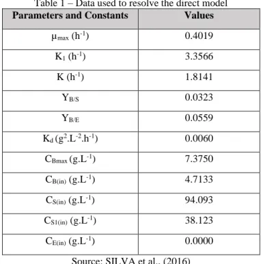
To solve the direct problem, the data of the reference parameters and constants were obtained from the data performed by the work of Silva et al. (2016), these data are summarized in Table 1.

Table 1 – Data used to resolve the direct model

Parameters and Constants Values

µmax (h-1) 0.4019 K1 (h-1) 3.3566 K (h-1₎ _1.8141 YB/S 0.0323 YB/E 0.0559 Kd (g2.L-2.h-1) 0.0060 CBmax (g.L-1) 7.3750 CB(in) (g.L-1) 4.7133 CS(in) (g.L-1) 94.093 CS1(in) (g.L-1) 38.123 CE(in) (g.L-1) 0.0000

Source: SILVA et al., (2016)

The simulated measurements were performed from the resolution of the direct model. It was adopted random data acquisition from a Gaussian distribution, with an average obtained from the direct model and standard deviation of 2% of the value maximum of the state variable. Thus, it was possible to obtain simulated measurements for each state variable in relation to time, this data collection was important to compare with the data obtained by solving the inverse problem.

(6)

3 INVERSE PROBLEM

3.1 SENSITIVITY ANALYSIS

According to Harrison (2017), a parameter is generally any characteristic that can help in the definition or evaluation of a system's performance. In this sense, the author registers that changes in the values of the parameters can correspond to changes in the behavior of the system, and such correspondence allows the possibility to track changes over time or in the experimental condition.

Another aspect is that the sensitivity coefficient analysis serves as an auxiliary tool for defining criteria for experimental projects, such as, for example, indicating which state variables are most significant for identifying parameters over time, in addition to defining a rate of frequency over time for the acquisition of experimental data as a function of the information gain to be obtained.

According to Özişik and Orlande (2000), the sensitivity matrix J is written according to Equation (8).

( )

T T P P C P J           = (8)

The sensitivity matrix is written as:

( )

T N I I I I N N P C P C P C P C P C P C P C P C P C P C P C P C P J                                             = L M M M M L L 3 2 1 2 3 2 2 2 1 2 1 1 1 1 1 1 1 (9)

The elements of the sensitivity matrix are called sensitivity coefficients, according to Equation (10). j i j i P C J   = , (10)

(7)

Braz. J. of Develop.,Curitiba, v. 6, n.5, p.26496-26516 may. 2020. ISSN 2525-8761 Ji,j is the sensitivity coefficient, C it represents the concentration vector, Pj represents

the parameters, I is the number of transient measurements and N is the number of unknown parameters.

The reduced sensitivity coefficients, represented by Equation (10), they are obtained by multiplying the original sensitivity coefficients by the parameter to which they refer. The use of reduced sensitivity coefficients is preferred for problems involving parameters with small orders of magnitude and in the identification of linear dependence. This is the case, because the reduced sensitivity coefficients can be directly compared in magnitude to the measured variables (ÖZIŞIK; ORLANDE, 2000; COSTA; NAVEIRA-COTTA, 2019).

j i j j i P C P x   = , (11)

In this step the objective is: to identify the parameters which, when applying a certain disturbance, generate significant magnitudes of variation in the system; identify and eliminate linearly dependent parameters with other parameters.

To calculate the reduced sensitivity coefficients (Equation 11), finite difference approximations were used for first order central derivatives, described in Equation (12). Where ε is the disturbance in the parameter and Np is the total number of parameters.

(

)

(

)

  2 , , , , , , , , ₂ ₁ ₂ 1 , Np j i Np j j i j i P P P P C P P P P P C x  L + − L (12)

Before addressing the estimation of unknown parameters, it is necessary to analyze the behavior of the determinant of the information matrix |JT_{J|, in order to inspect the influence of}

the number of parameters to be estimated in the solution of the inverse problem (ÖZIŞIK; ORLANDE, 2000; NAVEIRA-COTTA; COTTA; ORLANDE, 2011).

Small magnitudes of the sensitivity coefficients or columns linearly dependent on the sensitivity matrix satisfy the problem of |JTJ| ≈ 0, in this case, the inverse problem is considered to be poorly conditioned (ÖZIŞIK; ORLANDE, 2000; ORLANDE et al., 2011). In order to have a greater maximization of |JTJ|, it is desirable to have sensitivity coefficients with large magnitudes and to be linearly independent, this is important for there to be a precise estimate

(8)

Braz. J. of Develop.,Curitiba, v. 6, n.5, p.26496-26516 may. 2020. ISSN 2525-8761 of the parameters (ORLANDE et al., 2011, COSTA; COTTA, 2019; NAVEIRA-COTTA; NAVEIRA-COTTA; ORLANDE, 2011).

3.2 MÉTODO MONTE CARLOS VIA CADEIA DE MARKOV (MCMC)

According to Müller (2011) the Markov Chain Monte Carlo Method (MCMC) uses computational simulation of the Markov chains in the parameter space. Maltby (2019) adds that a Markov chain is a mathematical system that experiences transitions from one state to another according to certain probabilistic rules, in addition, no matter how the process reaches its current state, possible future states will be corrected, depending exclusively on the current state and the elapsed time.

Müller (2011) also notes that Markov chains allow the use of ergodic averages to approximate the desired later expectations. In this sense, Costa and Naviera-Cotta (2019) points out that the MCMC can be used to extract samples of all possible parameters, so that the inference in the later probability becomes inference in the samples.

To solve the inverse problem, the Bayesian interference structure was adopted, using the the Markov Chain Monte Carlo Method, among the various existing approaches to implement the posterior simulation based on the punctual assessment of the previous distribution and the probability function. Bayes' theorem is declared as (KAIPO; SOMERSALO, 2005; MAYBECK, 1979):

( )

(

)

( ) (

)

( )

Y P Y P Y P P priore posteriori _     = | = | (13)

Y is Measurements vector, πprosteriori (P) is the posterior probabilistic density, πpriori (P)

is the prior probabilistic density for the parameters; π(Y|P) is the likelihood function; π(Y) is the probability density of the measurements that represents a normalization constant.

Assuming that the measurement errors are Gaussian random variables with zero mean, it is known the covariance matrix W and that the measurement errors are additive and independent of the P parameters, the likelihood function can be expressed by Equation (13) (COSTA; NAVEIRA-COTTA, 2019; KAIPO; SOMERSALO, 2005; MAYBECK, 1979).

(

) ( )



( )





( )



     ₋ ₋ ₋ = − − − P F Y W P F Y W P Y 12 12 T 1 2 1 exp 2 |   (14)

(9)

Braz. J. of Develop.,Curitiba, v. 6, n.5, p.26496-26516 may. 2020. ISSN 2525-8761 The MCMC algorithm used to explore the posterior distribution is the one proposed by Metropolis and Hastings (ORLANDE et al., 2011; GAMERMAN, 1997; METROPOLIS; ROSENBLUTH; TELLER, 1953). To implement the Markov chain, a density p (P*, P(t-1)) is needed, which provides the probability of changing from the current state of the chain, P(t-1), to the new state, P*. After selecting the proposal distribution, the Metropolis-Hastings sampling algorithm can be implemented by repeating the following steps (COSTA; NAVEIRA-COTTA, 2019, ESTUMANO et al., 2015; NAVEIRA-COTTA; COTTA; ORLANDE, 2010):

1. Select a candidate P* in the distribution p(P*, P(t-1)), where the proposal of a candidate in the Markov chain is based on the random walk model with Gaussian distribution, as follows:

P* =P( )t−1 +P( )t−1 (15)

ξ is a random variable generated from a normal distribution with zero mean and unit standard deviation and ω is the search step;

2. Calculate the probability of acceptance α:

(

)

( )

(

)

( )

(

)

(

( )

)

      = ₋* −_*1 *₋₁ | | | | , 1 min _t _q _t t P P p Y P P P p Y P    (16)

3. A random number U is generated from a uniform distribution, that is, U~U(0.1); 4. If U ≤ α, the new value Pt_{= P}*_{is accepted. Otherwise, P}t_{= P}(t − 1)_;

5. Go back to step 1

To verify the influence of the definitions adopted in the MCMC, the following variations were made and their results were compared:

- Variation of the initial estimate of each parameter, for this the exact value was multiplied by the following factors: 1000; 100; 10; 5; 2.

- Variation in the time interval for data acquisition: 60 minutes, 30 minutes; 15 minutes; 6 minutes;

- Variation in the acquisition of state variables: Y = [CS1], Y = [CS1 CE] e Y = [CS CS1

(10)

Braz. J. of Develop.,Curitiba, v. 6, n.5, p.26496-26516 may. 2020. ISSN 2525-8761 - Standard deviation variation: 20%; 10%; 5%; 2%; 1% in relation to the maximum of the state variables that were considered measures.

After generating MCMC results, their residual analysis was performed, through the difference between the reference values and the values generated by the MCMC over time.

4 RESULTS AND DISCUSSION

4.1 SENSITIVITY ANALYSIS

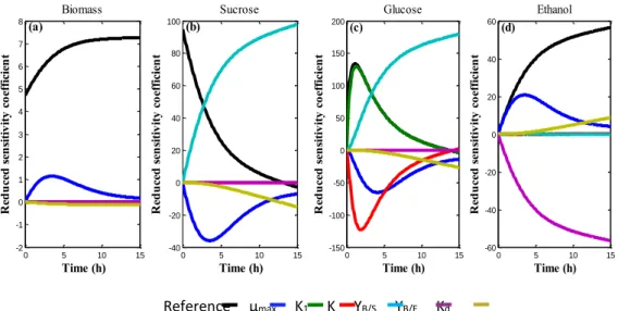
Through the sensitivity analysis it was possible to evaluate the linear dependence between parameters and their magnitudes. Based on these criteria, as can be seen in Figure 1a-d, parameters with significant magnitudes and linearly independent were define1a-d, namely: µmax, K1, YB/S, YB/E.

Figure 1 – Reduced sensitivity coefficient: Biomass (a); Sucrose (b); Glucose (c); ethanol (d)

Reference µmax K1 K YB/S YB/E Kd

Regarding glucose, K1 and K were linearly dependent, thus, observing the magnitudes

of their respective values, it was chose K1 as a parameter to be analyzed, due to its greater

amplitudes compared to K. In the parameter µmax, the magnitude of the reduced sensitivity

coefficient was significant for all state variables.

Only in ethanol it was possible to verify significant amplitudes of YB/E. The YB/S

parameter showed significant amplitudes only in the concentrations of sucrose and ethanol. Kd did not present significant magnitude values in any of the studied variables. The amplitudes

0 5 10 15 -2 -1 0 1 2 3 4 5 6 7 8 Time (h) R ed u ce d s en si ti vi ty c oe ff ic ie n t Biomass (a) 0 5 10 15 -40 -20 0 20 40 60 80 100 Time (h) R ed u ce d s en si ti vi ty c oe ff ic ie n t Sucrose (b) 0 5 10 15 -150 -100 -50 0 50 100 150 200 Time (h) R ed u ce d s en si ti v it y c o ef fi ci en t Glucose (c) 0 5 10 15 -60 -40 -20 0 20 40 60 Time (h) R ed u ce d s en si ti v it y c o ef fi ci en t Ethanol (d)

(11)

Braz. J. of Develop.,Curitiba, v. 6, n.5, p.26496-26516 may. 2020. ISSN 2525-8761 of all the analyzed parameters were significant up to the time of approximately 13 hours. In addition, after this period, it was observed that the parameters become linearly dependent.

With this result, it was initially expected that the concentrations of glucose and ethanol could obtain the parameters defined as significant and linearly independent (µmax, K1, YB/S,

YB/E).

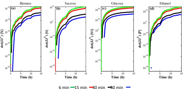
Figure 2a-d shows the determinant matrices for the state variables, adopting only the parameters (µmax, K1, YB/S, YB/E). Regarding the frequency of data capture over time, the

information gain was evaluated by varying this frequency in the following values: every 60 minutes; every 30 minutes; every 15 minutes; every 6 minutes. It was observed that the acquisition frequency in time around 15 minutes showed results close to those of 6 minutes. Glucose and ethanol achieved the highest values of |JTJ|, which corroborates with the results obtained by the reduced sensitivity coefficients.

Figure 2 – Determinant matrix: Biomass (a); Sucrose(b); Glucose (c); Ethanol (d).

6 min 15 min 30 min 60 min

4.2 MCMC ANALYSIS

Figures 3-6 show the MCMC analysis to estimate the parameters (µmax, K1, YB/S, YB/E).

It was applied in this analysis: variations in the standard deviation; data acquisition through state variables; frequency in time for data acquisition; variations in the initial estimate value. The number of states of the Markov chain was 10,000 interactions in all analyzes of parameter estimates. The values used as a reference for the parameters are described in Table 1.

The influence of state variables (Y = [CS1], Y = [CS1 CE] e Y = [CS CS1 CE CB]) was

studied. All combinations showed good convergence to obtain the selected parameters, except

0 5 10 15 10-60 10-50 10-40 10-30 10-20 10-10 Time (h) d et (J J T ) [X ] Biomass (a) 0 5 10 15 10-30 10-20 10-10 100 1010 Time (h) d et (J J T ) [S ] Sucrose (b) 0 5 10 15 10-30 10-20 10-10 100 1010 1020 Time (h) d et (J J T ) [S 1] Glucose (c) 0 5 10 15 10-40 10-30 10-20 10-10 100 1010 Time (h) d et (J J T ) [P ] Ethanol (d)

(12)

Braz. J. of Develop.,Curitiba, v. 6, n.5, p.26496-26516 may. 2020. ISSN 2525-8761 for the parameters acquisition through glucose (Y = [CS1]), which did not achieve good

convergence in capturing the YB/E parameter, due to the low magnitude of the parameter in

this variable, as shown in the sensitivity analysis (Figure 1d). This low convergence can be resolved by increasing the number of interactions of the Markov chain.

Figure 3 – MCMC considering measures in Y= [CS1], Y= [CS1 CE] and Y= [CB CS CS1 CE]: µmax (a); K1 (b); YB/S

(c); YB/E (d).

Reference [CS1] [CS1 CE] [CB CS CS1 CE

Figure 4a-d refers to the time frequencies for data acquisition, with intervals of 60, 30, 10, 1 and 0.5 minutes. With the exception of the 60-minute interval, the other frequencies (30, 10, 1, 0.5 minutes) achieved good convergence to obtain the studied parameters.

Figure 5a-d shows the tests in the Markov chain with different values of standard deviation. The deviation was calculated using the maximum value of state variable and applying 20%, 10%, 5%, 2 %, 1% in each case. Deviation values less than 5% obtained values closer to the references, as seen in Figure 5a-d. Better results were obtained close to 2% and 1% of deviation.

Figure 6a-d shows the tests with different values for the initial estimate value. The initial values were 1000, 100, 10, 5 and 2 times the reference value. Initial values with less

0 5000 10000 0.2 0.4 0.6 0.8 1  max Interation number (a) 0 5000 10000 3 4 5 6 7 K 1 Interation number (b) 0 5000 10000 0.02 0.04 0.06 0.08 Y B/ S Interation number (c) 0 5000 10000 0 0.05 0.1 0.15 0.2 Y B/ E Interation number (d)

(13)

Braz. J. of Develop.,Curitiba, v. 6, n.5, p.26496-26516 may. 2020. ISSN 2525-8761 than 10 times the reference value obtained convergences closer to the reference values in smaller numbers of interactions, as seen in Figure 6

Figure 4 – MCMC considering different measurement frequencies: µmax(a); K1(b); YB/S(c); YB/E(d).

Reference 60 30 10 1 0.5

Figure 5 – Parameters acquisition by changing the standard deviation: µmax (a); K1 (b); YB/S (c); YB/E (d).

Reference 20% 10% 5% 2% 1% 0 5000 10000 0.2 0.4 0.6 0.8 1  max Interation number (a) 0 5000 10000 3 4 5 6 7 K 1 Interation number (b) 0 5000 10000 0.02 0.04 0.06 0.08 Y B/ S Interation number (c) 0 5000 10000 0.04 0.06 0.08 0.1 0.12 Y B/ E Interation number (d) 0 5000 10000 0.2 0.4 0.6 0.8 1  max Interation number (a) 0 5000 10000 2 4 6 8 K 1 Interation number (b) 0 5000 10000 0.02 0.04 0.06 0.08 Y B/ S Interation number (c) 0 5000 10000 0.04 0.06 0.08 0.1 0.12 Y B/ E Interation number (d)

(14)

Braz. J. of Develop.,Curitiba, v. 6, n.5, p.26496-26516 may. 2020. ISSN 2525-8761 Figure 6 – Parameters acquisition by changing the initial estimate: µmax(a), K1(b), YB/S(c) e YB/E(d).

Reference 1000 100 10 5 2

4.3 CHOICE OF PARAMETERS

Based on the MCMC analysis (see figures 3-6), it is assumed for the optimized model: 10,000 states in the Markov chain; 2% standard deviation of the maximum value of state variables; measurement of parameters through the glucose and ethanol concentrations; initial estimate equal to twice the exact parameter value; 10 minute data frequency acquisition. Figure 7a-d shows the optimized model using the MCMC analysis. It was possible to verify in the figures that there was a convergence of the values of the parameters close to the reference values. 0 5000 10000 0 200 400  max Interation number (a) 0 5000 10000 0 1000 2000 3000 K 1 Interation number (b) 0 5000 10000 0 10 20 30 Y B/ S Interation number (c) 0 5000 10000 0 20 40 Y B/ E Interation number (d)

(15)

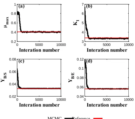
Braz. J. of Develop.,Curitiba, v. 6, n.5, p.26496-26516 may. 2020. ISSN 2525-8761 Figure 7 – MCMC model using the definitions adopted: µmax(a), K1(b), YB/S(c) e YB/E(d).

MCMC Reference

Table 2 compares the values of the reference parameters and the estimated ones, the relative error and quantiles at 99%. A satisfactory accuracy is perceived in the values generated compared to their reference values.

Table 2 – Reference and estimated parameters

Parameters Reference values Estimated values Relative error % Quantis 99%

µmax 0.4019 0.4012 0.1787 (0.3898; 0.4121)

K1 3.3566 3.3159 1.2134 (3.2513; 3.3698)

YB/S 0.0323 0.0324 0.3967 (0.0322; 0.0327)

YB/E 0.0559 0.0558 0.1018 (0.0554; 0.0564)

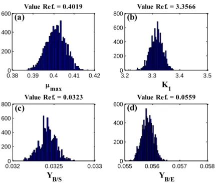
The histograms for the selected parameters were obtained (Figure 8). It is observed that the histograms of the parameters resemble Gaussian distributions with mean in the reference value. 0 5000 10000 0.2 0.4 0.6 0.8 1  max Interation number (a) 0 5000 10000 3 4 5 6 7 K 1 Interation number (b) 0 5000 10000 0.02 0.04 0.06 0.08 Y B/ S Interation number (c) 0 5000 10000 0.04 0.06 0.08 0.1 0.12 Y B/ E Interation number (d)

(16)

Braz. J. of Develop.,Curitiba, v. 6, n.5, p.26496-26516 may. 2020. ISSN 2525-8761 Figure 8 – Parameter histogram: µmax (a); K1 (b); YB/S (c); YB/E (d).

The model with the optimized parameters obtained good convergence with the data from the simulated measurement, for the concentrations of glucose (Figure 9c) and ethanol (Figure 9d), whose combinations obtained the best results for the acquisition of parameters. The model was also able to estimate values for the concentrations of Biomass and Sucrose, described in figures 9a-b.

Figure 9 – Direct model and MCMC for state variables: Biomass (a); Sucrose (b); Glucose (c); Ethanol (d).

Estimated Simulated measure

0.380 0.39 0.4 0.41 0.42 200 400 600 _max Value Ref. = 0.4019 (a) 3.2 3.3 3.4 3.5 0 200 400 600 800 K₁ Value Ref. = 3.3566 (b) 0.0320 0.0325 0.033 200 400 600 800 Y_B/S Value Ref. = 0.0323 (c) 0.0550 0.056 0.057 0.058 200 400 600 Y_B/E Value Ref. = 0.0559 (d) 0 5 10 15 4 5 6 7 8 Time (h) B io m as s (g /L ) (a) 0 5 10 15 -50 0 50 100 Time (h) S uc ro se (g /L ) (b) 0 5 10 15 0 50 100 Time (h) G lu co se (g /L ) (c) 0 5 10 15 0 20 40 Time (h) E th an ol (g /L ) (d)

(17)

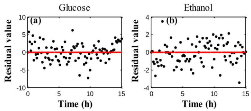
Braz. J. of Develop.,Curitiba, v. 6, n.5, p.26496-26516 may. 2020. ISSN 2525-8761 The residual analysis was calculated for glucose (CS1) and ethanol (CE) - state variables

determined to be significant. The residual values are the difference between the reference values and the values obtained by generating the model. It is observed the low magnitude of the residual values, compared to the magnitudes of the concentrations of glucose and ethanol. It indicates the possible correlation between the results and confirming that the proposed model is adequate to estimate the parameters that involve the fermentation process.

Figure 10 – Residual analysis: Glucose (a); Ethanol (b).

5 CONCLUSIONS

Based on experimental simulated measurement data for state variables Biomass (CB),

Sucrose (CS), Glucose (CS1) and Ethanol (CE) and performing simulated measurements with

the hypothesis of Gaussian distribution for likelihood and priori, it was defined as significant parameters, through the study of sensitivity analysis: maximum kinetics (µmax); kinetic

constant K1; substrate to product conversion factor (YB/E); and substrate conversion factor to

biomass (YB/S). In addition, continuing with the study of reduced sensitivity analysis, with the

aid of a determinant matrix for various combinations of concentration measurements, measurements through glucose and ethanol concentrations were defined as satisfactory to obtain such parameters.

After this step, performing the parameter estimates using the Markov Chain Monte Carlo Method with the Metropolis-Hastings acceptance and rejection algorithm. Variations in the standard deviation, initial estimate of the parameters, frequency of data acquisition and in the state variables were applied. The objective was to identify the best parameters values that would produce results more adjusted to the reference values. So it was obtained: 2% standard deviation of the maximum value of state variables; data acquisition through glucose and

0 5 10 15 -10 -5 0 5 10 Time (h) R es id u al v al u e Glucose (a) 0 5 10 15 -4 -2 0 2 4 Time (h) R es id u al v al u e Ethanol (b)

(18)

Braz. J. of Develop.,Curitiba, v. 6, n.5, p.26496-26516 may. 2020. ISSN 2525-8761 ethanol status variables; 10,000 states in the Markov chain; initial estimate equal to 2; 10 minutes for data acquisition frequency.

In all cases evaluated, good estimates of the parameters were obtained when comparing the estimates with the reference values. In addition to these estimates, analysis of the residues was carried out and it was found that it was at least one order of magnitude lower than the state variable that was simulated measured.

REFERENCES

CHOHAN, N.A., ARUWAJOYE, G.S., SEWSYNKER-SUKAI, Y., KANA, E.G. Valorisation of potato peel wastes for bioethanol production using simultaneous saccharification and fermentation: Process optimization and kinetic assessment. Renewable

Energy, v. 146, p. 1031-1040, 2020.

COSTA JR, J.M. NAVEIRA-COTTA, C.P. Estimation of kinetic coefficients in micro-reactors for biodiesel synthesis: Bayesian inference with reduced mass transfer model.

Chemical Engineering Research and Design, v. 141, p. 550-565, 2019.

DODIĆ, J.M.; VUČUROVIĆ, D.G.; DODIĆ, S.N.; GRAHOVAC, J.A.; POPOV, S.D.; NEDELJKOVIĆ, N.M. Kinetic modelling of batch ethanol production from sugar beet raw juice. Applied energy, v. 99, p. 192-197, 2012.

ESTUMANO, D.C.; BENK, E.; CARVALHO, R.C.; ORLANDE, H.R.B.; COLAÇO, M.J.; RIERA, J.J. Application of the Markov Chain Monte Carlo Method To Parameter Estimation in a Model Representing the Calcium Induced Calcium Release Mechanism in Neurons.

ABCM International Congress of Mechanical Engineering. 2015.

FOGLER, H.S. Elementos de Engenharia das Reações Químicas. 4o ed. Rio de Janeiro: LTC, 2009.

FONTOURA, C.R.O., ASEVEDO, S.D.M.L., NETO, M.R.F., SANTOS, L.M.R., PEREIRA, C.D.S.S. Uso do simulador de processos no estudo da engenharia química: uma aplicação no processo de produção de cerveja/Using the process simulator in chemical engineering study: an application in the beer production process. Brazilian Journal of Development, v.5, n. 8, p. 11724-11745, 2019.

(19)

Braz. J. of Develop.,Curitiba, v. 6, n.5, p.26496-26516 may. 2020. ISSN 2525-8761 GAMERMAN, D. Markov Chain Monte Carlo: Stochastic simulation for Bayesian

Inference. 1o ed. London: Chapman & Hall. 1997.

HARRISON, H.S. Multi-Level Dynamical Parameter Estimation: Hypothesis Testing

with Dynamical Systems. Doctoral Dissertations. University of Connecticut, 2017.

KAIPO, J.; SOMERSALO, E. Statistical and computational inverse problems. New York: Springer-Verlag; 2005.

LIMA, U.A.; AQUARONE, E.; BORZANE, W.; SCHMIDEL, W. Biotcnologia industrial:

Processos Fermentativos e enzimáticos. Volume 3. São Paulo: Edgard Bluncher, 2001.

MALTBY, H., PAKORNRAT, W., JACKSON, J., HERNANDEZ, A., WILLIAMS, C., LIN, C., KHIM, J. Markov Chains. Disponível em: https://brilliant.org/wiki/markov-chains/. Acesso em: 11/12/2019.

MAYBECK, P. Stochastic models, estimation and control. Academic, New York. 1979. METROPOLIS, N.; ROSENBLUTH, A.W.; TELLER, M.N. Equation of state calculations by fast computing machines. J. Chem. Phys. v 21, p. 1087–1092, 1953.

MÜLLER, P. Markov Chain Monte Carlo Methods. International Encyclopedia of the

Social & Behavioral Sciences, p. 9236-9240, 2011.

NAVEIRA-COTTA, C.P.; COTTA, R.M.E ORLANDE, H.R.B. “Estimation of space

variable thermophysical properties”. In: ORLANDE, H.R.B., FUDYM, O., MAILLEt, D.,

COTTA, R.M. (Org.), Thermal Measurements and Inverse Techniques. New York: CRC Press, p. 675–707, 2011.

NAVEIRA-COTTA, C.P.; COTTA, R.M.; ORLANDE, H.R.B. Inverse analysis of forced convection in micro-channels with slip flow via integral transforms and Bayesian inference.

International Journal of Thermal Sciences, v. 49, n. 6, p. 879-888, 2010.

NUNES, T.S., FINZER, J.R.D. A importância do tratamento do caldo de cana-de-açúcar para a produção de açúcar e etanol/The importance of sugar cane treatment for sugar and ethanol production. Brazilian Journal of Development, v. 5, n. 11, p. 24816-24823, 2019.

(20)

Braz. J. of Develop.,Curitiba, v. 6, n.5, p.26496-26516 may. 2020. ISSN 2525-8761 OLIVEIRA, S.C.; OLIVEIRA, R.C.; TACIN, M.V.; GATTÁS, E.A.L. Kinetic modeling and optimization of a batch ethanol fermentation process. J. Bioprocess. Biotech. 2016, v. 6, p. 266, 2016.

ORLANDE, H.R.B.; FUDYM, O.; MAILLET, D.; COTTA, R.M. (Org.). Thermal

Measurements and Inverse Techniques. New York: CRC Press, p. 675–707, 2011.

ÖZIŞIK, M.N.; ORLANDE, H.R.B. Inverse Heat Transfer: Fundamentals and

Applications. Taylor & Francis, 2000.

PASQUALETTE, M.A. ; ESTUMANO, D.C. ; HAMILTON, F.C. ; COLAÇO, M.J. ; LEIROZ, A.J.K. ; ORLANDE, H.R.B. ; CARVALHO, R.N. ; DULIKRAVICH, G.S. Bayesian estimate of pre-mixed and diffusive rate of heat release phases in marine diesel engines. Journal of the Brazilian Society of Mechanical Sciences and Engineering, v. 4, p. 1/655-10, 2016.

PASSOS, K. L. M., VIEGAS, B. M., MACÊDO, E. N., SOUZA, J. A. S., MAGALHÃES, E. M. Mathematical Modeling of Leaching Process of Red Mud in Order to Obtain the Kinetics Parameters. Revista de Engenharia Térmica, v. 14, n. 2, p. 90-94, 2015.

SANTOS, F. A.; QUEIRÓZ, J. D.; COLODETTE, J. L.; FERNANDES, S. A.; GUIMARÃES, V. M.; REZENDE, S. T. Potencial da palha de cana-de-açúcar para produção de etanol. Química nova, v. 35, n. 5, p. 1004-1010, 2012.

SARAWAN, C., SUINYUY, T. N., SEWSYNKER-SUKAI, Y., & GUEGUIM, E. K. Optimized activated charcoal detoxification of acid-pretreated lignocellulosic substrate and assessment for bioethanol production. Bioresource technology, v. 286, p. 121403-121403, 2019.

SILVA, C. L.; SANTANA, P. L. SILVA, C. F.; PAGANO, R. L. Modelagem e estimação de parâmetros do processo de produção de etanol em reator batelada por Saccharomyces cerevisiae. Scientia Plena. v. 12, n. 05, 2016.

SOMBRA, T. R., NUNES, M. P. M., SERRÃO, G. X., ARAÚJO, J. C., SOUSA, M. A. P., MORAIS, E. C., MACIEL, A. G. Utilização de redes bayesianas através do algoritmo naïve bayes para classificação de carcaças de ovinos/Use of bayesian networks through the na dove

(21)

Braz. J. of Develop.,Curitiba, v. 6, n.5, p.26496-26516 may. 2020. ISSN 2525-8761 bayes algorithm for the classification of sheep carcases. Brazilian Journal of Development, v. 6, n. 3, p. 10476-10498, 2020.

WANG, F. S., SHEU, J. W. Multiobjective parameter estimation problems of fermentation processes using a high ethanol tolerance yeast. Chemical Engineering Science, v. 55, n. 18, p. 3685-3695, 2000.

ZENTOU, H., ABIDIN, Z. Z., YUNUS, R., BIAK, A., RADIAH, D., ZOUANTI, M., HASSANI, A. (2019). Modelling of Molasses Fermentation for Bioethanol Production: A Comparative Investigation of Monod and Andrews Models Accuracy Assessment.