ANALYSIS OF TIME DOMAIN MCSEM DATA IN THE PRESENCE OF RESISTIVE LAYERS
Diego da Costa Miranda and C´ıcero Roberto Teixeira R´egis
Recebido em 2 outubro, 2009 / Aceito em 31 agosto, 2012 Received on October 2, 2009 / Accepted on August 31, 2012
ABSTRACT.Modeling of mCSEM data is usually done in the frequency domain, from its theoretical formulation to the analysis of the results. However, the time domain approach is, in principle, capable of providing equivalent information about the geo-electric structure of the subsurface and has the advantage of recording only the secondary fields, so the signal is not dominated by the primary field. In this work, we model frequency domain mCSEM data in 1-D environments, then we perform the discrete Fourier transform to obtain time domain results. We simulated marine geological environments with and without the resistive layer that represents the hydrocarbon reservoir. We verified that, in almost all model configurations, the time domain data are significantly different when calculated for models with and without hydrocarbons. We calculated the results considering variations in the position of the receivers and in the sea depth. We observed the influence of the airwave, even at large sea depths, and although a simple separation of this influence on data is not possible, the time domain results allowed us to do a qualitative analysis of its effects on the survey.
Keywords: time domain, mCSEM, Sea Bed Logging, discrete Fourier transform.
RESUMO.A modelagem do mCSEM ´e feita normalmente no dom´ınio da frequˆencia, desde sua formulac¸˜ao te´orica at´e a an´alise dos resultados. No entanto, a abordagem atrav´es do dom´ınio do tempo pode, em princ´ıpio, fornecer informac¸˜ao equivalente sobre a geof´ısica da subsuperf´ıcie aos dados no dom´ınio da frequˆencia, al´em de possuir a vantagem de registrar apenas o campo secund´ario, assim o sinal n˜ao ´e dominado pelo campo prim´ario. Neste trabalho, modelamos o mCSEM no dom´ınio da frequˆencia em modelos unidimensionais, e usamos a transformada discreta de Fourier para obter os dados no dom´ınio do tempo. Simulamos ambientes geol´ogicos marinhos com e sem uma camada resistiva, que representa um reservat´orio de hidrocarbonetos. Verificamos que os dados no dom´ınio do tempo apresentam diferenc¸as quando calculados para os modelos com e sem hidrocarbonetos em praticamente todas as configurac¸˜oes de modelo. Calculamos os resultados considerando variac¸˜oes na posic¸˜ao dos receptores e na profundidade do mar. Observamos a influˆencia daairwave, presente mesmo em modelos com grandes profundidades oceˆanicas, e apesar de n˜ao ser poss´ıvel uma simples separac¸˜ao dessa influˆencia nos dados, o dom´ınio do tempo nos permitiu fazer uma an´alise mais qualitativa de seus efeitos sobre o levantamento.
Palavras-chave: dom´ınio do tempo, mCSEM,Sea Bed Logging, transformada discreta de Fourier.
Universidade Federal do Par´a, Rua Augusto Corrˆea, 1, Guam´a, Caixa Postal 479, 66075-110 Bel´em, PA, Brazil. Phone: +55(91) 3201-7000 – E-mails: [email protected]; [email protected]
“main” — 2013/4/11 — 16:07 — page 302 — #2
302
ANALYSIS OF TIME DOMAIN MCSEM DATA IN THE PRESENCE OF RESISTIVE LAYERS INTRODUCTIONThe marine controlled-source electromagnetic (mCSEM, also known as Sea Bed Logging – SBL), has recently become a tool for exploration and mapping offshore hydrocarbon reservoirs, due to the need for risk reduction in exploration that led the oil indus-try to find news alternatives of prospecting. This has been made possible because of the improvement in the equipment and elec-tronics during the almost three decades in which the marine EM methods have been developed (Christensen & Dodds, 2007).
The mCSEM is a method for detection and characterization of thin resistive structures, like hydrocarbon reservoirs, usually lo-cated in regions of deep water (Eidesmo et al., 2002). It consists of a mobile horizontal electric dipole as a source, carried close to the seafloor where an array of electromagnetic receivers are deployed. The dipole transmitter emits a low frequency signal, that spreads both in the water and in the sediments beneath it and is captured by the receivers, as shown in Figure 1. Amplitude and phase of this signal depend on the electrical resistivity of the seafloor and seawater parameters. A recent overview of the method is provided, for example, by Frenkel & Davydycheva (2012).
The mCSEM modelling consists in the computational simula-tion of the geological environments of which we want informasimula-tion. It is an important task, because it allows an a priori study, indicat-ing the best conditions for the surveys.
Modelling of mCSEM is usually done in the frequency do-main, due to simplifications that are possible when we work with low frequencies. One of them is the fact that Maxwell’s equations become easier to be solved, since we do not deal with the time derivatives. However, time domain data may provide information on the geophysical characteristics of the subsurface that is equiv-alent to frequency domain data (Constable & Srnka, 2007).
EM time domain approaches show up very well adapted in land surveys, where the geological formations are on the con-ductive side of the air/earth system. In marine environments, the system is inversed, and the region of interest becomes the most resistive, i.e., the ocean subsoil, which is more resistive than the seawater. So, the information about the seafloor occurs in the early time response while the seawater response dominates later time. This separation of the responses is an appreciable feature of the time domain method and cannot be easily observed in the frequency domain. A comparative study of the two approaches is provided by Avdeeva et al. (2007). In addition, efficient ap-plications of time domain methods can be found for example in Oldenburg et al. (2007), B¨orner et al. (2008) and Afanasjew et al. (2008).
Because the time domain method is only measuring the sec-ondary field, it offers a solution to the shallow water limitations, where the frequency-targeted techniques have great difficulty to operate due to the strong downward field that is generated at the air/sea interface (Strack et al., 2008).
In this paper, we calculate the time domain mCSEM data from 1-D frequency domain modelling using the discrete Fourier trans-form, with models that contain or not the resistive layer which represents the hydrocarbon reservoir.
Our research supports that the time domain mCSEM approach is feasible, although we use simplified geological models which do not correspond to all the features of real environments. The 1-D electromagnetic modelling, however, is essential to obtain initial information, like the primary EM field in a stratified medium, that can help us with more complex problems, such as those involving 2-D and 3-D modelling.
METHODOLOGY Theoretical revision
The decay in the amplitude and the phase shift of the signal are both controlled by the geometric effect and the skindepth (Um & Alumbaugh, 2007). The geometric effect yields a field decay that is related to the kind of source that generates the signal. The skindepth is a measure of the field decay related to the sig-nal frequency and the electrical properties of the medium. The skindepth is generally described as:
δ= s
2 ωμσ
where ω is the angular frequency and μ is the magnetic perme-ability.
So, a distance of several skindepths between source and re-ceiver may cause the captured signal to be dominated by the sed-iments response, since in the seawater the skindepth is usually smaller than in the sediments.
The mCSEM is based on the contrast of resistivity between the marine geological environments and the saturated hydrocar-bon reservoirs possibly present in these locations. A reservoir filled with oil for instance, can have a resistivity up to 100 times higher than the area around it, usually dominated by shale and saline fluids. Thus, a survey using various transmitters and vari-ous receiver positions can determine a multidimensional resistive model of the ocean subsurface (Eidesmo et al., 2002).
In time domain mCSEM, we use a time variant electromag-netic field as source that induces eddy currents within the sedi-ment layers. These eddy currents are also time variant and they
Figure 1 – Scheme of a geophysics survey using mCSEM.
produce a secondary field that can be sensed by the electromag-netic receivers. Depending on the subseafloor geological tures, these fields can be more or less disturbed. In general, struc-tures with greater resistivity are responsable for the greater distur-bances and the signal transmitted by the source travels faster in them (Constable & Srnka, 2007).
But, the received signal is also composed by fields that prop-agated directly through the seawater and by fields that have in-teracted with the atmosphere (which are commonly known as air-wave). Because the electrical conductivity of the seawater is usu-ally greater than the seafloor, the response of the seawater comes later than the seafloor, and the arrival time and amplitude of the airwave will depending primarily on the seadepth (Constable & Srnka, 2007).
So, by the analysis of the time-dependent curve, we can dis-tinctly observe the seawater and the seafloor responses. Although the same procedure cannot be done with the airwave response, in some cases, we can at least find the location in time where this influence is higher. Such a diagnostic is not easy to do in the frequency-domain although it contains the same information as the time domain data.
1-D modelling
For the 1-D problem, we use the formulation based on the de-composition of the primary signal in flat waves and the Schel-kunof Potentials to obtain the electric field in the receivers (Ward & Hohmann, 1988). We start from Maxwell’s Equations in the
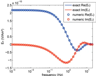
frequency domain, obtaining values that represent the radial elec-tric field. To calibrate our program, we approximated the mCSEM geoelectrical model for a homogeneous formation and compared the results with the exact solution of this problem, which can be found in, for instance, Ward & Hohmann (1988). Figure 2 shows the exact and numerical frequency domain solutions for theEx normalized by the dipole moment of the source, measured by a single receiver in a homogeneous formation with resistivity of ρ= 1m and distance of 900 m from the transmitter.
Figure 2 – Real (blue) and imaginary (red) part ofExfor various frequencies
in a homogenous medium.
To obtain the time domain solution, we need to perform the discrete Fourier transform and this implies in calculating the responses for a large number of frequencies. The details of the
“main” — 2013/4/11 — 16:07 — page 304 — #4
304
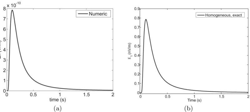
ANALYSIS OF TIME DOMAIN MCSEM DATA IN THE PRESENCE OF RESISTIVE LAYERSFigure 3 – Program validation. Comparison of our result (a) with the result presented by Mulder et al. (2008) (b) both using a homogenous medium.
discrete Fourier transform applied in our frequency data can be found in Miranda (2007). Naturally, the use of such a number of frequencies increases the computational time of the task. For a 1-D model this is not necessarily an issue, but for 2-D and 3-D models, it can be a very demanding problem. To address this problem, we also adapted our code to run in parallel machines. We have used the parallel environment provided by the Netuno cluster, located at the Universidade Federal do Rio de Janeiro (UFRJ). Thus, the task could be divided (we distributed the cal-culations for various frequencies among the Netuno’s execution nodes), decreasing the total execution time. Working with paral-lel computing will be our best choice when we apply our code to 2-D models in our next research phase.
We study two different functions representing the current in the source: an impulse function, representing a sudden increase and decrease in the current in a very short time and a step func-tion, representing a current that is turned suddenly on and remains steady for a long time. The second one, where the input function of the source is a Heaviside function, provides information about the time evolution of the system in such a way that allows us to make a normalization of the responses, by dividing the result of a particular model by another, so we can get a curve of the anomaly due to the differences between the geologic models.
To check our time domain result, we compared the impulse response of the horizontal electric dipole in a homogeneous for-mation obtained by numerical modelling with the exact time so-lution of this problem presented by Mulder et al. (2008), at a distance of 900 m from the transmitter, as shown in Figure 3.
RESULTS
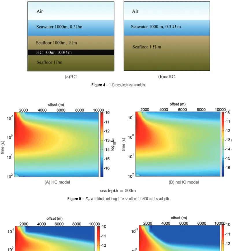
We use the models presented by Constable & Weiss (2006) showed in Figure 4. The model called HC has a hydrocarbon reservoir with a resistivity of 100m and thickness of 100 m, buried at a depth of 1000 m between sediments of resistivity of 1m. The sea has resistivity of 0.3m and depth of 1000 m. The model called noHC is similar to the previous, but it has no resistive layer.
The results below are the time domain solution obtained by discrete Fourier transform of the frequency domain data.
Figures 5, 6 and 7 show the time domain amplitudes of Exviewed as colormaps relating time × offset for seadepths of 500 m, 1000 m and infinite, considering an impulse function as source waveform.
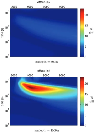
Figure 8 shows the relative difference (rd) (rd = 100 × |1− HC/noHC|) between HC and noHC curves for seadepths of 500 m and 1000 m respectively.
We can observe that, for distances closer to the transmit-ter, the signal looks similar in all sections. This is because, for a very short offset the response from sediments arrives before the direct response (signal that travels through the water) gets decayed. As we consider larger offsets, like 4 km or more, we noticed greater differences between the HC and noHC results. Distances, like 10 km, presents very weak signals, whose am-plitudes are in the range of the geological noise. So, we can as-sume that a distance of 5 km is well suited for the time domain measurements for this model and it was the offset used in the next results.
Figure 4 – 1-D geoelectrical models.
Figure 5 –Examplitude relating time × offset for 500 m of seadepth.
“main” — 2013/4/11 — 16:07 — page 306 — #6
306
ANALYSIS OF TIME DOMAIN MCSEM DATA IN THE PRESENCE OF RESISTIVE LAYERSFigure 7 –Examplitude relating time × offset for an infinite seadepth.
Figure 8 – Relative difference between HC and noHC curves for seadepths of
500 m and 1000 m.
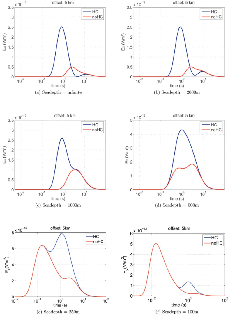
Figure 9 shows the amplitude of theExcomponent for sea-depths of 100 m, 250 m, 500 m, 1000 m, 2000 m and an in-finite seadepth, at an offset of 5 km using the same source as the previous example, where we can observe the effects due to the changes of seadepth. The seadepth controls the rate of
in-fluence of the fields that interacted with the atmosphere in the results. The shallower the sea, the smaller the attenuation of these fields, also called airwave.
Although it is not possible a simple separation of the air-wave in the results, the curves showed in Figure 9 provide in-formation about its interaction with the geological environments. Figure 9(a) shows the electrical response of the sediments with-out any airwave influence, since we have an infinite seadepth which completely attenuates this response. In the HC curve of the same Figure, we can see two peaks, the first with amplitude of 2,5 × 10⁻¹³V/m2and the second with amplitude of 0,125 × 10−13V/m2approximately. Since the signal going through the sediments have been spread in a more resistive medium than the seawater, its arrives first, making us conclude that the peak of greater amplitude is the sediments response. So, the lower peak would be the seawater response, that is, the signal that propagates only through the seawater.
Looking at Figure 9(b), with the results for the model with 2000 m of seadepth, we noticed a slight increase in amplitude for both HC and noHC results, around the time of 5 seconds, indicat-ing the region of influence of the airwave.
Figure 9(c) shows the result for 1000 m of seadepth and we can observe striking changes not only in the shapes of the curves but also in their amplitudes when compared with the previous ex-amples. For this model, the airwave effect occurs earlier than in the model with greater seadepths, coinciding with the time re-sponse of the sediment without the resistive layer.
A similar analysis can be done in Figure 9(d) correspond-ing to the model with 500 m of seadepth. In this example we observed a strong influence of the airwave. Comparing the red
“main” — 2013/4/11 — 16:07 — page 308 — #8
308
ANALYSIS OF TIME DOMAIN MCSEM DATA IN THE PRESENCE OF RESISTIVE LAYERScurve of this graph, related to the noHC model, with the noHC curves of the other models, we can infer that the first of the two peaks in Figure 9(d) is due to the direct response of the airwave, and the second peak is due to the seafloor response, which is also affected by the airwave. This is because the time response of the sediment without the resistive layer is almost the same in all graphs. In the blue curve of Figure 9(d), it is not possible to distinguish these peaks, because there is an overlap between the responses of the airwave and the sediments.
Figures 9(e) and 9(f) show the results for the models with 250 m and 100 m of seadepth respectively, which correspond to what is usually called shallow water (seadepths less than 500 m) by the geophysicists. In these Figures, we can notice a stronger influence of the airwave than in the previous examples, charac-terized by the large amplitude of the earlier peaks that appears in each of the curves of both Figures. Because these peaks occur in a quite different time than that of the sediment response, the sig-natures of resistive structures are not masked, indicating that the method can be used even in shallow water environments.
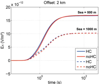
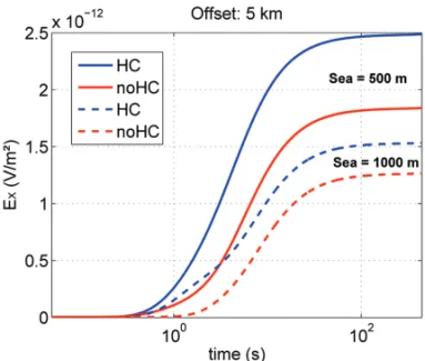
Figures 10 and 12 display the step response for receivers lo-cated at 2000 m and 5000 m from the source, respectively, con-sidering seadepths of 500 m, 1000 m and 2000 m. Figures 11 and 13 display the same HC data normalized by the correspond-ing noHC response.
In the normalized curves we have a measure of the relative influence of the resistive layer on the data. The lower peak in the 2 km offset shows a strong influence of the field directly from the source, which is greater than the influence of the re-sistive layer as well as of the air-water interface. When the off-set is 5 km the peaks are higher than before, which shows that the resistive layer is felt more strongly, while the direct field from the source is relatively weaker. Also, note that the influence of the air-water interface is increased, since now the curves for the depths of 1000 m and 2000 m are clearly separated, which was not the case in the 2 km offset.
CONCLUSION
The results show that meaningful information about the geoelec-trical structure under the sea can be inferred from time domain mCSEM data. Because the measurements are done with the di-pole source turned off, the method has the potential to detect weak reservoir responses or, as in the case of shallow water, it provides that the signal can be separated from the airwave sponse. In regions of greater seadepths, the air interaction re-sponse takes a longer time to reach the receiver and can
over-ride the seafloor response or even intensify it, since this down-ward signal can spread in the sediments also. Furthermore, we observed relevant differences between the resistive and conduc-tive curves corresponding to the HC and noHC models respec-tively in all seadepths that we have tested, for the two kinds of source waveforms used. In the sequence of this research, we will investigate the information that can be gathered from 2-D and 3-D models, by formulating the problem in the time domain from first principles.
ACKNOWLEDGMENTS
We thank PETROBRAS and the N´ucleo de Computac¸˜ao Eletrˆonica (NCE) of the Universidade Federal do Rio de Janeiro (UFRJ) for the use of the Netuno cluster. We also thank the CNPq for the scholarship that supported this research.
Figure 10 – Time-domain solution for the step response at a source-receiver
distance of 2000 m.
Figure 11 – Normalized solution for the step response at a source-receiver
Figure 12 – Time-domain solution for the step response at a source-receiver
distance of 5000 m.
Figure 13 – Normalized solution for the step response at a source-receiver
dis-tance of 5000 m. REFERENCES
AFANASJEW M, EIERMANN M, ERNST OG & G ¨UTTEL S. 2008. Im-plementation of a restarted krylov subspace method for the evalu-ation of matrix functions. Linear Algebra and its Applicevalu-ations, 429: 2293–2314.
AVDEEVA A, COMMER M & NEWMAN GA. 2007. Hydrocarbon reser-voir detectability study for marine CSEM methods: time-domainversus frequency-domain. SEG/San Antonio 2007 Annual Meeting. Expanded Abstract, pp. 628–632.
B¨ORNER R-U, ERNST OG & SPITZER K. 2008. Fast 3-D simulation of transient electromagnetic fields by model reduction in the frequency do-main using Krylov subspace projection. Geophysical Journal Interna-tional, 173: 766–780.
CHRISTENSEN NB & DODDS K. 2007. Marine controlled-source electro-magnetic methods 1D inversion and resolution analysis of marine CSEM data. Geophysics, 72: WA27–WA38.
CONSTABLE S & SRNKA LJ. 2007. An introduction to marine controlled-source electromagnetic methods for hydrocarbon exploration. Geo-physics, 72: WA3–WA12.
CONSTABLE S & WEISS CJ. 2006. Mapping thin resistors and hydro-carbons with marine em methods: Insights from 1D modeling. Geo-physics, 71: G43–G51.
EIDESMO T, ELLINGSRUND S, MACGREGOR LM, CONSTABLE S, SINHA MC, JOHANSEN S, KONG FN & WESTERDAHL H. 2002. Sea Bed Logging (SBL), a new method for remote and direct identifica-tion of hydrocarbon filled layers in deepwater areas. First Break, 20: 144–152.
FRENKEL MA & DAVYDYCHEVA S. 2012. To CSEM or not to CSEM? Feasibility of 3D marine CSEM for detecting small targets. Leading Edge, 31(4): 435–446.
MIRANDA DC. 2007. Modelagem do mCSEM no dom´ınio do tempo usando transformada discreta de Fourier. Master’s thesis, Universidade Federal do Par´a. Available on: <http://www.cpgf.ufpa.br>. Access on: October 10, 2012.
MULDER WA, WIRIANTO M & SLOB EC. 2008. Time-domain modeling of electromagnetic diffusion with a frequency-domain code. Geophysics, 73: F1–F8.
OLDENBURG DW, HABER E & SHEKHTMAN R. 2007. Rapid forward modelling of multi-source TEM data. Proceedings of the 4thInternational Symposium on Three-Dimensional Electromagnetics, pp. 35–38. STRACK K, ALLEGAR N & ELLINGSRUD S. 2008. Marine time domain CSEM: an emerging technology. SEG/Las Vegas 2008 Annual Meeting. Expanded Abstract, p. 653.
UM ES & ALUMBAUGH DL. 2007. On the physics of the marine controlled-source electromagnetic method. Geophysics, 72: WA13– WA26.
WARD SH & HOHMANN GW. 1988. Electromagnetic theory for geophys-ical applications. In: NABIGHIAN M (Ed.), Electromagnetic methods in applied geophysics, volume 1, chapter 4. Society of Exploration Geo-physicists, 131–311.
“main” — 2013/4/11 — 16:07 — page 310 — #10
310
ANALYSIS OF TIME DOMAIN MCSEM DATA IN THE PRESENCE OF RESISTIVE LAYERS NOTES ABOUT THE AUTHORSDiego da Costa Miranda has a Physics degree (2007) and a M.Sc. in Geophysics (2009) both from the Universidade Federal do Par´a, UFPA, Brazil. He is currently a
Ph.D. student at the Graduate Program of Geophysics from the Federal University of Par´a, working on the following topics: electromagnetic methods, modeling of Marine Controlled-Source Electromagnetic and parallel processing.
C´ıcero Roberto Teixeira R´egis got a doctorate in Geophysics from the Universidade Federal do Par´a, UFPA, Brazil, in 1999. He has been teaching Math and Physics,
at the secondary and university levels, since 1992. He is member of the Faculty of Geophysics in the UFPA since 2004. His research includes the numerical modeling and inversion of electromagnetic marine geophysical methods.