www.scielo.br/rbg
APPLICATION OF A SPATIAL VERIFICATION METHOD TO GFS PRECIPITATION FORECASTS
Fabiani Denise Bender and Rita Yuri Ynoue
ABSTRACT.This study aims to describe a spatial analysis of precipitation field with the MODE tool, which consists in comparing features converted from gridded forecast and observed precipitation values. This evaluation was performed daily from April 2010 to March 2011, for the 36-h GFS precipitation forecast started at 00 UTC over the state of S˜ao Paulo and neighborhood. Besides traditional verification measures, such as accuracy (A), critical success index (CSI), bias (BIAS), probability of detection (POD), and false alarm ratio (FAR); new verification measures are proposed, such as area ratio (AR), centroid distance (CD) and 50th and 90th percentiles ratio of intensity (PR50 and PR90). Better performance was attained during the rainy season. Part of the errors in the simulations was due to overestimation of the forecasted intensity and precipitation areas.
Keywords: object-based verification, weather forecast, precipitation, MODE, S˜ao Paulo.
RESUMO.Este estudo tem como objetivo descrever uma an´alise espacial do campo de precipitac¸˜ao com a ferramenta MODE, que consiste em converter valores de precipitac¸˜ao de grade do campo previsto e observado em objetos, que posteriormente ser˜ao comparados entre si. A avaliac¸˜ao ´e realizada diariamente sobre o estado de S˜ao Paulo e vizinhanc¸a, para o per´ıodo de abril de 2010 a marc¸o de 2011, para as simulac¸˜oes do modelo GFS iniciadas `as 00 UTC, na integrac¸˜ao de 36 horas. Al´em da verificac¸˜ao atrav´es de ´ındices tradicionais, como probabilidade de acerto (PA), ´ındice cr´ıtico de sucesso (ICS), vi´es (VI´ES), probabilidade de detecc¸˜ao (PD) e raz˜ao de falso alarme (RFA), novos ´ındices de avaliac¸˜ao s˜ao propostos, como raz˜ao de ´area (RA), distˆancia do centroide (DC) e raz˜ao dos percentis 50 e 90 de intensidade (RP50 e RP90). O melhor desempenho ocorreu para a estac¸˜ao chuvosa. Parte dos erros nas simulac¸˜oes foi devido `a superestimativa da intensidade e da ´area de abrangˆencia dos eventos de precipitac¸˜ao em relac¸˜ao ao observado.
Palavras-chave: avaliac¸˜ao baseada em objetos, previs˜ao do tempo, precipitac¸˜ao, MODE, S˜ao Paulo.
Universidade de S˜ao Paulo, Instituto de Astronomia, Geof´ısica e Ciˆencias Atmosf´ericas, Departamento de Ciˆencias Atmosf´ericas, Rua do Mat˜ao, 1226, Cidade Univer-sit´aria, 05508-090 S˜ao Paulo, SP, Brazil. Phone: +55(11) 3091-4712 – E-mails: [email protected]; [email protected]
INTRODUCTION
Verification techniques for the spatial field of precipitation have been typically based on grid overlays in which the forecast grid is matched to an observation grid or a set of observation points and from these overlays, the pair of forecast/observation is compared and evaluated using categories defined by a 2×2 contingency table (Wilks, 2006). The performance of the numerical weather prediction model is then determined by a variety of traditional ver-ification measures such as probability of detection, false alarm ratio, and critical success index, in which the hits and misses of precipitation are based on the presence or absence of rain event.
It is known that precipitation is highly discontinuous in space and time (Casati et al., 2004) and due to significant spatial vari-ability; their structure and specific location can be difficult to forecast (Brown et al., 2007; Biazeto & Silva Dias, 2012). Some of the difficulties associated with prediction diagnostic errors using traditional approaches for the verification of spatial forecasts have been described by Davis et al. (2006a-b). Therefore, traditional verification measures usually reduce the performance of forecast. In this context, the Method for Object-based Diagnostic Eval-uation (MODE) has been suggested as a technique to be applied to the analysis of the precipitation field. This verification tool for the evaluation of precipitation fields is an “Object-based” ap-proach, in which forecast and observed areas of precipitation are represented and compared as objects, and characterized by at-tributes such as location, size, and intensity of the systems (Davis et al., 2006a; Brown et al., 2007; Davis et al., 2009). Besides, MODE is publicly available at the Model Evaluation Tools website (MET – www.dtcenter.org/met/users).
Most studies in the literature apply precipitation verification indices for a few days only. It is known in operational meteorology centers that models tend to have better performances during some seasons of the year, especially during the summer rainy months. Greater errors are usually found on spring and autumn. This study aims to add quantitative verification of the Global Forecast Sys-tem (GFS) to the S˜ao Paulo state for a one year period. This paper describes an application of Method for Object-based Diagnostic Evaluation (MODE) and its application for the verification of spa-tial precipitation forecast. Section 2 presents a brief description of the GFS model and the verification tool applied in this study; the predicted and observed data used in the application of MODE; an example of object-identification approach to one forecast and observed precipitation field; and some verification measures ana-lyzed. Section 3 presents results, with a daily analysis for January and July, and then, a monthly analysis for the traditional and new measures. Finally, in Section 4 there is a synthesis of the results and we present our conclusions.
METHODOLOGY GFS Model
GFS is a weather forecast global spectral model and is run op-erationally since 1991 at the National Centers for Environmental Prediction (NCEP, Kanamitsu, 1989; Kalnay et al., 1990; Kana-mitsu et al., 1991). It is run four times a day at 00, 06, 12 and 18 UTC but for this work only the forecast initiated at 00 UTC and 3-hour forecast outputs for the first 36 hours with a hori-zontal resolution of 1◦of latitude× 1◦ of longitude was con-sidered. The main parameterizations may be listed as: i) Pan & Wu (1995) deep convection parameterization, which is acti-vated when the cloud work function exceeds a certain threshold; ii) Han & Pan (2011) shallow convection scheme, which uses a bulk mass-flux parameterization; iii) Grid-scale condensation and precipitation, which are based on Zhao & Carr (1997); iv) Planetary Boundary Layer processes follow Troen & Mahrt (1986); and v) Rapid Radiative Transfer Model for long (Mlawer et al., 1997) and shortwave (Hou et al., 2002) radiation. Changes are continuously made and annual reviews are available for 2009 to 2013. These evaluations however, are made either within a global perspective, showing, for example, hemispheric performance for 500 hPa geopotential height forecasts or at a local perspective, presenting precipitation performance for the Continental U.S.A. These reviews and more details can also be found at GFS home-page (http://www.emc.ncep.noaa.gov/GFS/.php).
MODE
MODE is applied in the following order: conversion of gridded precipitation values of forecast and observed field into precipi-tation objects; definition of measurement attributes for forecast and observed objects; merging of objects in the same field; matching of objects from the forecast and observed fields; com-parison of forecast and observed object attributes and summary of the results.
The object identification involves two parameters. First, a convolution ratio R is applied to the data field, which consists in smoothing the raw data using a convolution filter. The second parameter is a threshold, T, which is applied to the convolved field to create objects that look similar to those which a human eye would draw. The choice of parameter T depends on whether we are interested in more or less intense precipitation areas. Once the objects have been identified, various attributes are assigned for categorization and evaluation. A fuzzy logic process is used for the merging and matching of objects, in which weightings are assigned to the different attributes. As a result, values of interest
are defined, which range between 0 and 1, with zero indicating no interest, and one indicating strong interest. Finally, pairs of objects which have values above the threshold are merged (if the objects are in the same field) or matched (if they are in dif-ferent fields).
MODE was applied to evaluate daily rainfall accumulation (mm, at synoptic time 12 UTC) from 01/04/2010 to 31/03/2011 at S˜ao Paulo state, Brazil. Comparisons were made with the outputs from the 1◦× 1◦Global Forecast System (GFS) (NCEP, 2003) model, on a 36-h forecast initialized at 00 UTC. As gridded ob-servations, MERGE 0.25◦× 0.25◦fields (Rozante et al., 2010), which consists of a combination of the Tropical Rainfall Measur-ing Mission (TRMM) satellite precipitation estimates with surface observations over South America, were used. The study area has a high density of observations and according to Rozante et al. (2010) MERGE performance is equivalent to averaging stations data within the grid boxes.
For MODE evaluation, both observed and forecast fields were interpolated to a new grid with 0.25◦ of spatial resolution, on a domain from 53.6W to 43.6W of longitude and from 25.6S to 19.6S of latitude covering S˜ao Paulo state and neighborhood (Fig. 1). For object identification, the convolution radius R was set to 2 (grid units) and the threshold T was 0.3 mm.day–1. This
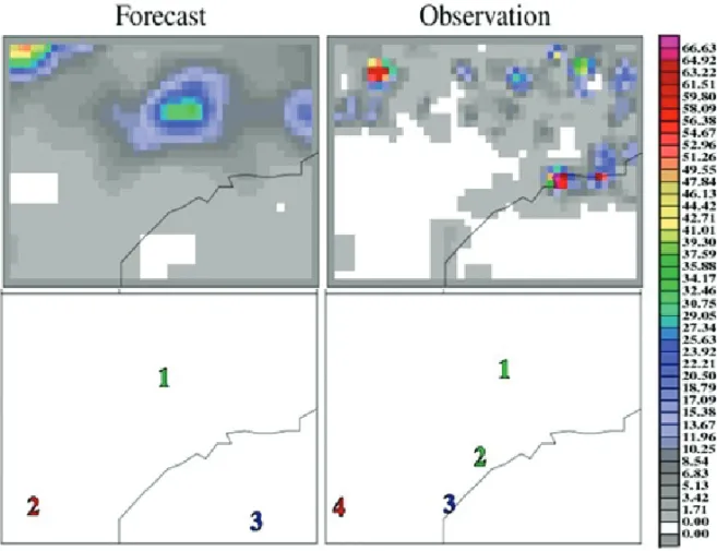
threshold was used by Chou & Justi da Silva (1999) for identifying rain events over South America’s. For the matching and merging processes an interest value greater than 0.7 was considered. a) An example of application: identification of objects Figure 2 (upper panel) shows the raw precipitation fields from GFS (left column) and MERGE (right column), valid for 1st April 2010 12 UTC, for the domain and spatial grid resolution considered in the application of MODE. The values shown are 24-h rainfall accumulations (mm). In Figure 2 (lower panel) we have the ob-jects identification after the application of convolution ratio and threshold to the raw fields. Three forecast objects and four ob-served objects were identified. Each rain area identified within the analysis field is referenced to as an object. Table 1 shows a matrix with total interest value for each forecast/observed object pair. We have assumed that a match occurs when the total interest is 0.7 or greater. Using this threshold, forecast object 1 matches observed objects 1 and 2 (therefore, observed objects 1 and 2 are merged). Forecast object 2 matches observed object 4. Forecast object 3 is unmatched, because total interest was less than 0.7, for all objects of the observed field. Each object is indicated by a distinct color, and those to be merged within the same field have the same color (Fig. 2, lower panel).
Table 1 – Interest matrix. Total interest values are computed for each forecast/observed object pair. Total interest values greater than 0.7 are shown in bold numbers in the matrix.
Observed Forecast 1 2 3 4 1 1 0.86 0.51 0.25 2 0.33 0.07 0.51 0.90 3 0.48 0.15 0.25 –
The next step is the consideration of objects within a polygon. A polygon is composed of a single object, or a combination of objects within the same field in which these objects have neces-sarily values of interest greater than 0.7 relative to at least one object of compared field. Thus, by definition, a polygon is a set of one or more objects in the same field, which is compared with a set of one or more objects in another field. The combination of objects considers that individual simple objects in the same field can be merged before comparison, thus forming a large compos-ite object.
Polygons are limited by lines and those polygons filled with the same color in predicted and observed fields indicate matched pairs of polygons. The comparisons are then done matching poly-gons of the predicted and observed fields.
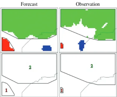
For this example, two pairs of polygons were compared (Fig. 3). The first pair, identified by a red color, is formed by one object of the forecast field in Figure 2 (red forecast object 2) and one object of the observed field (red observed object 4 in Fig. 2). The second pair identified by the green color, consists by the comparison of a single object from forecast field (green forecast object 1 in Fig. 2) with a composite of combined objects from the observed field (objects 1 and 2, both green in Fig. 2). Blue objects from forecast and observed fields were not merged or matched.
Table 2 presents some attributes of the polygons pairs com-pared shown in Figure 3. The first pair of matched polygons (red area) has an interest value of 0.90, while the second pair (green area) has an interest value equal to 0.95. For the first pair of matched polygons, the forecast area was 81 grid units, while the observed area showed 14 units grid, with area ratio of 5.79; in-dicating that the forecast highly overestimated the precipitation area. For the second pair of matched polygons the forecast area was closer to the observed area, with area ratio equal to 1.19.
Lower values for the centroid distance and the angular differ-ence, for the pair of second set of polygons, with values of 2.59 and 8.35, compared to the pair of the first set, with values equal to 2.69 and 30.72, indicates that the location and inclination of rainfall areas forecast for the second set was closer to the observation. Values of convex hull equal to 0 for the two pairs
Figure 1 – Domain used in the evaluation of precipitation fields simulated by the GFS with the MODE tool bounded by the rectangle.
Figure 2 – Spatial field of 24-h accumulated rainfall (mm) simulated by the GFS, in 36-h forecast (left); observed by MERGE (right), of 1 April 2010, both with spatial grids resolution and domain considered in MODE with a horizontal spatial resolution of 0.25◦ lati-tude/longitude (upper panel). Objects identified by MODE (lower panel).
of polygons, indicates an overlap of the polygons, with intersec-tions areas of 14 and 761 grid points.
Figure 3 – Forecast (left side) and observed (right side) rain objects identified by MODE, for a threshold of 0.3 mm and (lower panel) forecast and observed polygons identifications for total interest values> 0.7.
Finally, the GFS tended to overestimate precipitation inten-sity, for both the 50th (0.45 and 4.93 mm forecastedversus 0.32 and 2.36 mm observed for the 1st and 2nd pair of polygons re-spectively) and 90th (1.30 and 16.79 mm forecastedversus 1.08 and 16.06 mm observed for the 1st and 2nd pair of polygons respectively) percentile values. However, extreme values (90th percentile) were better predicted.
Table 2 – Attributes of polygons pairs matched between GFS forecast and MERGE observed fields for the case of 1 April 2010, shown in Figure 3.
Attributes Polygon pairs matched
1 2
Total interest 0.90 0.95
GFS area 81 943
MERGE area 14 790
Area Ratio (AR) 5.79 1.19
Intersection area 14 761
Union area 81 972
Centroid Distance (CD) 2.69 2.59
Convex Hull Distance 0 0 Angular Difference 30.72 8.35 GFS 50th Intensity 0.45 4.93 MERGE 50th Intensity 0.32 2.36 50th Percentile Ratio (PR50) 1.41 2.09 GFS 90th Intensity 1.30 16.79 MERGE 90th Intensity 1.08 16.06 90th Percentile Ratio (PR90) 1.20 1.05
b) An example of application: traditional and new verification measures
Figures 2 and 3, as described above, shows the objects and pairs of polygons identified for the predicted (left) and observed (right) field of daily rainfall accumulation on 1st April 2010. The traditional verification measures are calculated based on the rainfall areas identified after applying the parameters R and T, i.e. based on grid points of Figure 3 (upper panel). The new veri-fication measures suggested by MODE, area ratio, intersection and union areas, centroid and convex hull distances, angular dif-ferences, intensities and intensity ratios are calculated based on each matched pair polygons, corresponding to the internal region bounded by the black line, lower panel of.
The distribution of forecast and observed events can be de-fined based on four categorical forecasts in a contingency table: “a” number of event forecasts that is observed, usually called hits; “b” number of event forecasts that is not observed, called false alarm; “c” number of no-event forecasts corresponding to ob-served events, called misses; and “d” number of no-event fore-casts corresponding to no-events observed, called correct rejec-tion. Based on these categories the following verification mea-sures are defined as:
– Accuracy (A): total number of correct forecasts divided by the total number of forecasts, it is the percent of correct forecasts,A = (a + d)/(a + b + c + d).
– Critical Success Index (CSI): total number of correct event forecasts divided by the number of events forecasts and observed,CSI = (a)/(a + b + c).
– Bias (BIAS): total number of event forecast divided by the total number of observed events, BIAS = (a + b)/(a + c).
– Probability of detection (POD): number of correct event forecasts divided by the number of observed events, P OD = (a)/(a + c).
– False Alarm Ratio (FAR): number of false alarm divided by the total number of event forecasts, F AR = (b)/(a + b).
The new verification measurements made between matched pairs of polygons are: centroid distance (CD), area ratio (AR), and intensities for the 50th and 90th ratio percentiles (PR50 and PR90).
The traditional verification measures determined for this day are summarized in Table 3. The A is around 75%. The CSI varies
around 67%. The BIAS indicates overestimation of precipitation area of the order of 1.30. The POD shows performance in the order of 92% due to the fact that GFS forecasts precipitation over a large area, covering the area of observed precipitation. The FAR value is in the order of 30%.
Table 3 – Traditional verification measures index verified by MODE for the daily accumulation precipitation field of 1st April 2010, shown in Figure 3.
A CSI BIAS POD FAR 75% 67% 1.30 92% 30%
The new verification measures for this day were already shown in Table 2 and are highlighted in bold. The area ratio (AR) is overes-timated causing the displacement of centroid distance (CD) of the polygons pairs compared. This area overestimation would explain the traditional indices: high POD and low FAR, due to large num-ber of hits and low values of misses. Rainfall intensities are also compared with this new approach, although the traditional way could be done making contingency tables for different categories. RESULTS
a) Application of MODE for the daily forecasts of January and July
MODE was applied daily for a whole year period, from 1st April 2010 to 31st March 2011. An one year period is not enough to evaluate GFS performance, but since the objective of this study was to present a new precipitation verification method, during this year the rainy summer and dry winter seasons could be en-compassed. Here we show the daily evolution of statistical in-dices only for the months of January and July (Figs. 4, 5, 6 and 7), representative of rainy summer and dry winter months respectively.
In January, GFS showed good performance, with a success rate above optimal set for a useful forecast (60%, Fig. 4a). The lowest scores of A coincide with days on which has the low-est scores of CSI (Fig. 4b) and highlow-est BIAS (Fig. 4c) and FAR (Fig. 4e).
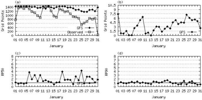
On Figure 5 we show the evolution of the daily new indices for the month of January. In Figure 5a, it is observed that the GFS model predicts events with larger spatial extent (in units of grid) in relation to the observed. This greater precipitation forecast area is found throughout the whole study period, as will be commented on Figure 8. The largest overestimation of areas coincide with the greater centroid distances between forecast/observed polygons pairs (Fig. 5b), explaining the lowest performance of the tradi-tional indices and also the good performance due to POD.
There-fore, the overestimation of the area and the displacement of the forecast events imply in a higher number of false alarms. Regard-ing the intensity of rainfall events, the events of weak to moderate intensity (PR50) showed an overestimation pattern (Fig. 5c), while events of higher intensities (RP90) tend to be forecasted near the observed intensities (Fig. 5d). It is interesting to notice that not only the area was overestimated, but also the intensity of rainfall, but the 90th, despite the larger area, was better estimate.
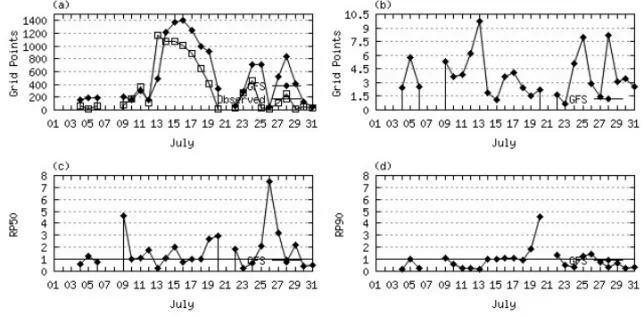
For the month of July, the traditional and new indices are shown in Figures 6 and 7, respectively. It is clear from both fig-ures that the model simulates better precipitation fields for the summer season. This is primarily due to fewer and weaker rain events occurring in smaller areas during the dry season. Index A (Fig. 6a) assumes on average values above 60%. The best scores of CSI occur on days from 14 to 18/07, when the indices of POD (Fig. 6b), BIAS (Fig. 6c) and FAR (Fig. 6e) have the best scores. By checking the new indices it is found that precipitation events forecast/observed had lower spatial extent in grid units (Fig. 7a) compared to the daily evolution of January. The best perfor-mance of the GFS, with higher CSI, POD and lower values of BIAS and FAR on days from 14 to 18 coincides with the period in which rainfall events had greater coverage area and therefore with lower values of the centroid distance (CD) (Fig. 7b), agree-ing with the fact that events with smaller spatial extent present greater difficulty to be predict correctly in terms of location, and thus have higher false alarms. In Figure 7d-e, the PR50 indicates overestimation of the intensities, while PR90 presents sometimes a pattern of overestimation and in other times an underestimation pattern, but with a ratio closer to unity.
Days in which the new performance measures were absent in the graphics are those without polygons pairs been compared. b) Monthly Mean Evolution
In order to quantify the annual oscillation of the verification sta-tistical indices evaluated, the monthly mean for each index was calculated and is shown in Figures 8 and 9, where monthly evolution refers to the average of the daily indices for the corre-sponding month.
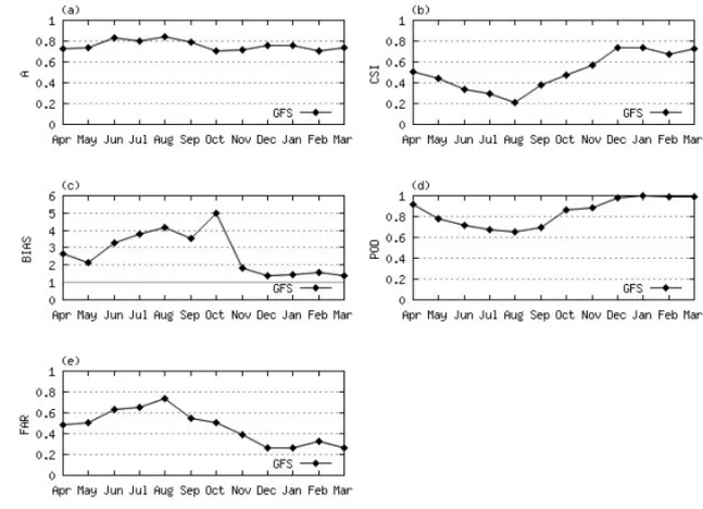
As Figure 8a shows, A, for each month evaluated, remained above 70%. In the months between May to September (dry sea-son, Prado et al., 2008) the A index was around 80%. CSI, by having a direct relationship with the occurrence of rain, presents satisfactory results, greater than 70%, in the summer rainy months (December to March), while the lowest levels, below 50%, occurring in the months of the dry season (May to Septem-ber) (as show in Fig. 8b), coinciding with the highest values
Figure 4 – Traditional verification indices, for the daily rainfall accumulation of GFS, in 36-h forecast, identified by MODE for January 2011. (a) Accuracy (A), (b) Critical Success Index (CSI), (c) Bias (BIAS), (d) Probability of Detection (POD), and (e) False Alarm Ratio (FAR).
Figure 5 – New verification measures index, for the daily rainfall accumulation of GFS, in 36-h forecast, identified by MODE for January 2011. (a) Number of grid points with precipitation, (b) Centroid Distance (CD), (c) 50th percentile ratio (PR50), and (d) 90th percentile ratio (PR90).
of BIAS (Fig. 8c), and FAR (Fig. 8e) and lowest scores of POD (Fig. 8d).
The GFS presented BIAS above 1, both in the dry and wet season, agreeing with McBride & Ebert (2010), who also found
a pattern of overestimation of precipitation area with respect to 7 operational models over Australia for one year period. The high-est values of overhigh-estimation (above 2) occurring from April to October, thus covering the entire period of the dry season (May to
Figure 6 – Traditional verification indices, for the daily rainfall accumulation of GFS, in 36-h forecast, identified by MODE for July 2010. (a) Accuracy (A), (b) Critical Success Index (CSI), (c) Bias (BIAS), (d) Probability of Detection (POD), and (e) False Alarm Ratio (FAR).
Figure 7 – New verification measures index, for the daily rainfall accumulation of GFS, in 36-h forecast, identified by MODE for July 2010. (a) Number of grid points with precipitation, (b) Centroid Distance (CD), (c) 50th percentile ratio (PR50), and (d) 90th percentile ratio (PR90).
September), with the maximum BIAS occurring on October. De-spite the overestimation in the summer months, the model has values close to the unity.
FAR values were below 30% in the months from December to March, i.e. in summer season. In the months between May to September, the FAR assumes the highest values, exceeding 50%, thus indicating that in this period the expected rainfall events, in
terms of area, presents a high risk of false alarm (Fig. 8e). The months from May to September (dry season) had the worst performance, with lower values of CSI, POD and a marked overestimation BIAS and high FAR. Thus, there is a need for adjustments in the microphysics and cumulus parameterization of the model, in order to have better performance in the region studied.
Figure 8 – Monthly mean traditional verification indices identified by MODE for period of April 2010 to March 2011. (a) Accuracy (A), (b) Critical Success Index (CSI), (c) Bias (BIAS), (d) Probability of Detection (POD), and (e) False Alarm Ratio (FAR).
Despite the small predictability for the period from May to September, highest values for A were observed. Although differ-ent reasons may explain the differences in precipitation, we can highlight two of them: the first, a higher frequency of days with-out rain predicted/observed, and the second, that both forecast and observed rain areas show little spatial area coverage. Thus, if the prediction and observation are presented in different loca-tions, although A is high, the FAR is also high, but CSI and POD are smaller.
Figure 9 shows the monthly evolution for the new verifica-tion measures proposed by MODE. It is observed that there are more grid points with precipitation predicted than observed for the whole period, with greatest areas from December to March covering the summer rainy season (Fig. 9a). However, greatest area ratio overestimate is found for the dry season, agreeing with the highest values of BIAS. The period with smaller rain-fall areas (from April to September), is the same one with longer distances between the centroids of pairs of forecast/observed
Figure 9 – Monthly mean new verification indices identified by MODE for the period of April 2010 to March 2011. (a) Number of grid points with precipitation, (b) Centroid Distance (CD), (c) 50th percentile ratio (PR50), and (d) 90th percentile ratio (PR90).
polygons (Fig. 9b), agreeing with the lower scores of CSI and POD and higher values of BIAS and FAR. The smaller distances from the centroid occurs during the rainy season; coinciding with larger coverage precipitation areas.
Interestingly, as was observed for the months of January and July, the 50th percentile on Figure 9c shows an overestimate for almost all the months evaluated. However, the 90th percentile is closer to the observation intensity. In general, models tend to overestimate the lowest precipitation intensities and underesti-mate the highest intensities (Cartwright & Krishnamurti, 2007).
CONCLUSIONS
This study presented an object-based approach for the evaluation of spatial forecast fields applied to daily accumulation rainfall during one year over S˜ao Paulo state, Brazil. Beyond traditional verifications measures, this new tool, MODE, is able to provide a large variety of information about the forecast performance.
Based on the traditional verification measures, it is concluded that the GFS has a reasonable representation when it takes into account the accuracy index. The best predictability index of rain-fall events occur in the months from December to March (JFM – summer season), with high values of CSI, POD and smaller BIAS and FAR. The new indices provide more information: there was an overestimation pattern in terms of spatial coverage, in grid units as in intensity of rain events. With regard to intensity, the 50th percentile simulated is generally larger than those observed; however, the 90th percentile is close to the observations. The new indices also show that the low scores of BIAS and FAR coincide with the dry season, when the precipitation events have lower spatial extent and are more difficult to be forecast in the right position.
The advantage of MODE use is that as an object-based met-ric, it allows to obtain a large variety of diagnostic and meaning-ful information about the performance of precipitation forecast. That is, while traditional statistics provide numbers that can be used to monitor a model forecast performance the new indices provide information about the way in which a forecast went wrong or did well.
ACKNOWLEDGEMENTS
The authors acknowledge the IAG/USP and CNPq for support during the development of the work. We thank Jos´e Roberto Rozante (CPTEC/INPE) for providing MERGE product data. We wish to thank the anonymous reviewers for their helpful com-ments, which allowed us to greatly improve the manuscript.
REFERENCES
BIAZETO B & SILVA DIAS MAF. 2012. Analysis of the impact of rainfall assimilation during LBA atmospheric mesoscale missions in Southwest Amazon. Atmos. Res., 107: 126–144.doi: 10.1016/j.atmosres.2012.01.004.
BROWN BG, BULLOCK R, HALLEY-GOTWAY J, AHIJEVYCH D, DAVIS C, GILLELAND E & HOLLAND L. 2007. Application of the MODE object-based verification tool for the evaluation of model precipita-tion fields. In: 22nd Conference on Weather Analysis and Forecast-ing and 18th Conference on Numerical Weather Prediction. June 25– 29, Park City, Utah. American Meteorological Society, Boston. Available on:<http://ams.confex.com/ams/pfdpapers/124856.pdf>. Access on: December 5, 2010.
CARTWRIGHT TJ & KRISHNAMURTI TN. 2007. Warm Season Meso-scale Superensemble Precipitation Forecasts in the Southeastern United States. Wea. Forecasting, 22: 873–886.
CASATI B, ROSS G & STEPHENSON DB. 2004. A new intensity-scale approach for the verification of spatial precipitation forecasts. Meteorol. Appl., 11: 141–154. doi: 10.1017/S1350482704001239.
CHOU SC & JUSTI DA SILVA MGA. 1999. Objective Evaluation of ETA Model Precipitation Forecast over South America. Revista Climan´alise, 1(1): 1–17.
DAVIS C, BROWN B & BULLOCK R. 2006a. Object-Based Verifica-tion of PrecipitaVerifica-tion Forecasts. Part I: Methodology and ApplicaVerifica-tion to Mesoscale Rain Areas. Mon. Wea. Rev., 134: 1772–1784.
DAVIS C, BROWN B & BULLOCK R. 2006b. Object-Based Verification of Precipitation Forecasts. Part II: Application to Convective Rain Systems. Mon. Wea. Rev., 134: 1785–1795.
DAVIS CA, BROWN BG, BULLOCK R & HALLEY-GOTWAY J. 2009. The Method for Object-Based Diagnostic Evaluation (MODE) Applied to Numerical Forecasts from the 2005 NSSL/SPC Spring Program. Wea. Forecasting, 24: 1252–1267.
HAN J & PAN H-L. 2011. Revision of Convection and Vertical Diffusion Schemes in the NCEP Global Forecast System. Wea. Forecasting, 26: 520–533.
HOU Y-T, MOORTHI S & CAMPANA K. 2002. Parameterization of solar radiation transfer in the NCEP models. NCEP Office Note 441. KALNAY E, KANAMITSU M & BAKER WE. 1990. Global numerical weather prediction at the National Meteorological Center. Bull. Amer. Meteor. Soc., 71: 1410–1428.
KANAMITSU M. 1989. Description of the NMC global data assimila-tion and forecast system. Wea. Forecasting, 4: 335–342.
KANAMITSU M, ALPERT JC, CAMPANA KA, CAPLAN PM, DEAVEN DG, IREDELL M, KATZ B, PAN HL, SELA J & WHITE GH. 1991. Re-cent changes implemented into the global forecast system at NMC. Wea. Forecasting, 6: 425–435.
McBRIDE JL & EBERT EE. 2010. Verification of Quantitative Precipita-tion Forecast from OperaPrecipita-tional Numerical Weather PredicPrecipita-tion Models over Australia. Wea. Forecasting, 15: 103–121.
MLAWER EJ, TAUBMAN SJ, BROWN PD, IACONO MJ & CLOUGH SA. 1997. Radiative transfer for inhomogeneous atmospheres: RRTM, a validated correlated-k model for the longwave. J. Geophys. Res., 102: 16663–16682.
NCEP – National Centers for Environmental Prediction. 2003. The GFS atmospheric model. NCEP Office Note 442, EMC/Global Climate and Weather Modeling Branch, Camp Springs, MD, 14 pp.
PAN H-L & WU W-S. 1995. Implementing a Mass Flux Convection Parameterization Package for the NMC Medium-Range Forecast Model. NMC Office Note, No. 409, 40 pp. [Available from NCEP, 5200 Auth Road, Washington, DC 20233].
PRADO LF, PEREIRA FILHO AJ, HALLAK R & LOBO GA. 2008. Organi-zac¸˜ao espacial da precipitac¸˜ao no Estado de S˜ao Paulo. In: Congresso Brasileiro de Meteorologia, S˜ao Paulo, Brazil, Proceedings..., 4 pp.
ROZANTE JR, MOREIRA DS, GONC¸ALVES LGG & VILA DA. 2010. Combining TRMM and Surface Observation Precipitation: Technique and Validation over South America. Wea. Forecasting, 25: 885–894. doi: 10.1175/2010WAF2222325.1.
TROEN I & MAHRT L. 1986. A simple model of the atmospheric bound-ary layer; Sensitivity to surface evaporation. Bound.-Layer Meteor., 37: 129–148.
WILKS DS. 2006. Statistical Methods in the Atmospheric Sciences. 2nd ed., Elsevier, 627 pp.
ZHAO QY & CARR FH. 1997. A prognostic cloud scheme for operational NWP models. Mon. Wea. Rev., 125: 1931–1953.
Recebido em 18 junho, 2013 / Aceito em 5 maio, 2014 Received on June 18, 2013 / Accepted on May 5, 2014
NOTES ABOUT THE AUTHORS
Fabiani Denise Bender. Bachelor’s degree in Meteorology (Universidade de Santa Maria – UFSM – 2010); Master degree in Atmospheric Sciences (Univer-sidade de S˜ao Paulo – USP – 2012). Currently, is a Ph.D. student at the Program in Agricultural Engineering (Escola Superior de Agricultura Luiz de Queiroz – ESALQ/USP). Develops research in impacts of climate changes on agriculture.
Rita Yuri Ynoue. Bachelor’s, Master’s and PhD’s degree in Meteorology (Universidade de S˜ao Paulo – USP – 1992, 1999 and 2004, respectively). Currently, is an Assistant Professor at Universidade de S˜ao Paulo with research emphasis on 1) Atmospheric Chemistry, acting on the following themes: urban air pollution and photochemical modeling emissions, ozone, aerosol urban size distribution of the particulate matter, and 2) Synoptic Meteorology, acting in numerical modeling.