Mining images of microbial communities for morphological characteristics in a support of clinical decision making

(1)

Universidade do Minho

Escola de Engenharia

Ana Catarina de Jesus Domingues

Mining images of microbial communities

for morphological characteristics in a

support of clinical decision making

(2)

(3)

Universidade do Minho

Dissertação de Mestrado

Escola de Engenharia

Departamento de Informática

Ana Catarina de Jesus Domingues

Mining images of microbial communities

for morphological characteristics in a

support of clinical decision making

Mestrado em Bioinformática

Trabalho realizado sob orientação de

Professora Doutora Anália Lourenço

Professora Doutora Maria Olívia Pereira

(4)

(5)

iii To my brother, António Domingues.

(6)

(7)

v

Acknowledgements

All my accomplishments in life are a result of my surroundings; therefore I am thankful for my dear friends, colleagues, and professors that made this journey possible.

To Professor Analia Lourenço for giving me this opportunity at the University of Vigo and for all the help and enlightenment during the past years. To Professor Maria Olivia Pereira, for her inexhaustible patience in answering my biological questions and giving me advice. To Ana Sousa, for the images and the biological insights. Professor Analia and Professor Olivia, you are an example to me.

I would also like to thank the Sing 33 group at University of Vigo, in particular Professor Florentino Riverola, Hector Vallejo, and Jeny Varela for making me feel at home. Thanks are also due to Nadine Santos, my partner in this adventure, for all the laughs.

I would like to dedicate this thesis to my brother António, my inspiration, my support. Thank you for challenging me to do this masters, and to not settle down in life. You are my mentor. Also, thanks to Andrea Freitag for all the love and support.

And finally, most importantly, my parents, António and Graciete. Obrigada por todo o amor e apoio incondicional, sem vocês eu não era nada.

(8)

(9)

vii

Resumo

Um biofilme é uma comunidade de microrganismos envoltos por uma matriz extracelular produzida pelos próprios, que lhes garante proteção. Os biofilmes representam um problema para a saúde pública pois facilmente encontram-se em dispositivos médicos, podendo causar problemas graves para os pacientes.

Estudos prévios indicam algumas alterações observáveis do aspeto físico e bioquímico das comunidades microbianas na resposta à resistência e à virulência. Assim a morfologia da comunidade pode ser um indicativo da reação regulatória associada com fenómenos de patogenicidade microbiana.

O objetivo deste trabalho é por um lado a criação de um novo sistema de classificação de morfologia de colonia com medidas extraídas de softwares de imagem por outro lado, o estudo da classificação morfológica existente e do novo sistema de classificação, através de técnicas de mineração de dados com o objetivo de ajudar nestas classificações. Apresentamos vários softwares como solução que vão desde a caraterização da estrutura dos biofilmes até a caraterização de morfologia de colonia

Palavras-chave: Biofilmes, morfologia de colonia, processamento de imagens, mineração de

(10)

(11)

ix

Abstract

Biofilms are communities of microorganisms embedded in a self-produced extracellular matrix, adherent to an inanimate, biotic surface that provides them with protection. Biofilms are a healthcare problem since they can be found in several medical devices and end up causing problems for the patients.

Previous studies have reported observable physical and biochemical changes of microbial communities associated with resistance and virulence response. This suggests that the morphology of a biofilm is a marker for regulatory interplays associated with the microbial phenomenon of pathogenicity.

The aims of this work are on the one hand, create a novel system of colony morphological classification with measurements extract from image software on the other hand study the current manual morphological classification and the novel one through data mining techniques. Here we present several software solutions to facilitate the process, from the determination of biofilm structure to the characterisation of colony morphology.

(12)

(13)

xi

List of Figures

Figure 1: The Biofilm Life Cycle... 7

Figure 2: Biofilms on different surfaces. ... 7

Figure 3: Common sites of biofilm infection in humans. ... 9

Figure 4: Several images relevant to the study of diseases associated with biofilms. ... 11

Figure 5 : Thresholding Algorithm Flowchart... 17

Figure 6: ImageJ interface. ... 26

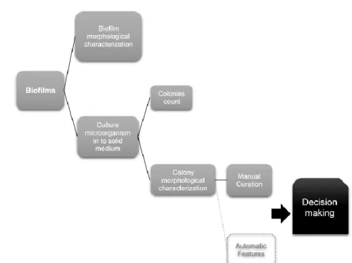
Figure 7: Generic workflow of biofilm characterization with the end goal but not yet created of clinical decision making. ... 33

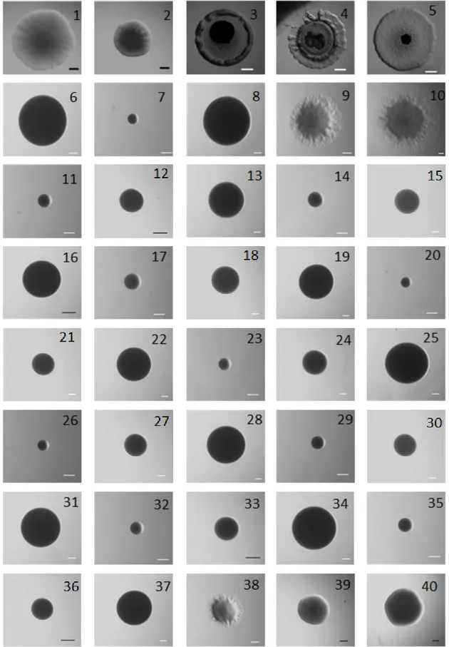
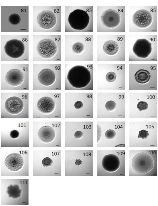
Figure 8: Full dataset of images used in this thesis work. ... 35

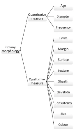
Figure 9: Colony Morphology according to http://miabie.org. ... 38

Figure 10: Detail of the manual curation measurements ... 39

Figure 11: Analysis pipeline in ImageJ, emphasising the pre-processing steps. ... 42

Figure 12: Description of the two regions in an image of the data set. ... 43

Figure 13: Surface profile plot of image1 (see also Figure 8 and Table 3)... 47

Figure 14: Diagram of the datasets that will be discussed during this chapter... 53

Figure 15: Average value of each ImageJ measurement. ... 56

Figure 16: Images clustered in single-cluster by Euclidean K-means. ... 64

Figure 17: Images in Euclidian Distance cluster C15 that appear in separate Cosine Similarity clusters. ... 66

Figure 18: Distribution of images in ImageJ and manualC clusters generated with Euclidian distance. ... 69

Figure 19: Distribution of images in ImageJ and manualC clusters generated with Cosine similarity. ... 71

Figure 20: Images in unitary ManualC clusters (Cosine similarity)... 72

(16)

xiv

List of Tables

Table 1: Publicly available image analysis software tools for structural analysis of microorganism

aggregates... 25

Table 2: Publicly Available Image Analysis Software Tools for counting. ... 30

Table 3: Classification of all the colonies used in this study according to manual curation measurements - ManualC dataset (see images in Figure 8). ... 39

Table 4: Description of basic shape measurements obtained from ImageJ. ... 45

Table 5: Description of basic pixel value measurements from ImageJ. ... 45

Table 6: Examples of textural metrics provided by ImageJ. ... 46

Table 7: Examples of metrics outputted by the surface roughness in ImageJ... 47

Table 8: The top 15 ImageJ measurements selected by different algorithms in Weka... 49

Table 9: Measurement most frequently after performing analysis for attribute selection in Weka. ... 54

Table 10: Results of k-means partitioning for the ImageJ dataset. ... 60

Table 11: All the clustering results performed on the 2 datasets, with 2 different k-means algorithms. ... 61

Table 12: Euclidean distance clustering versus Cosine Similarity clustering. ... 66

Table 13: Assessment of Euclidian distance clustering quality representing the level of agreement between the annotations... 68

Table 14: Assessment of Cosine Similarity clustering quality representing the level of agreement between the annotations... 70

(17)

xv

Acronyms

AR Aspect Ratio

ASM Angular Second Moment

cir Circularity

CLSM Confocal Laser Scanning Microscopes

CVF Connected Volume Filtration

EPS Extracellular Polymeric Substances

FISH Fluorescence In Situ Hybridization

GFP Green Fluorescent Protein

GLCM Grey Level Co-Occurrence Matrix

IntDen Integrated Density

PCC Pair Cross-Correlation Function

Ra Roundness Average

ROI Region Of Interest

Round Roundness

Rq Root Mean Square

Rsk Skewness

Rsu Kurtosis

Stddev Standard Deviation

(18)

1. Introduction

1

Chapter 1. Introduction

1.1 Context and Motivation

Biofilms can be defined as aggregates of microorganisms embedded in a self-produced extracellular matrix and adhering to inanimate and biotic surfaces. Biofilms can be composed by one or more microbial species, but polymicrobial biofilms composed of several bacterial species are the most common [1]. Biofilms can also be formed by fungi microorganisms like Candida albicans. Besides the microorganisms, biofilms are also composed by interconnecting compounds which keep the microorganisms stuck to each other and to the surface. These compounds can be self-produced (such as polysaccharides, proteins, extracellular DNA and cell lysis products), substances derived from the immediate surrounding environment, or even dead cells [2].

Microorganisms within a biofilm can form long-term relationships, interacting with each other and establishing metabolic cooperation and/or antagonistic interactions. In a biofilm community, microorganisms tend to express different genes and proteins depending on the specific needs of particular biofilm region [3]. The genotype and phenotype alterations tend to be reflected in the morphology of the biofilm, i.e., the physical structure of the biofilm is somewhat reflective of how the biofilm cells interact with the environment [4]. Therefore, the capturing of images from different sections of the biofilm, with the corresponding quantification of the biofilm structure, is used to obtain insights about the biological processes that are taking place.

Furthermore, it is normal to culture microorganisms derived from biofilms onto solid media to characterize their growth patterns and to investigate their response to stimuli, such as their susceptibility profiles to antibiotic treatments. Culture onto solid media is a way to estimate the number of the associated cells and their ability to grow. Theoretically, one viable biofilm-associated cell can give rise to a visible colony through multiplication. The morphology adopted by the biofilm-derived colonies formed on the solid media can also provide important insights about biofilm resistance, virulence and pathogenicity. For that reason, the studies related to the

(19)

1. Introduction

2 observable physical and biochemical traits of both microbial aggregates, i.e. biofilms and colonies, are often associated.

Colony morphotyping is an emerging topic of research due to its potential implication in antimicrobial resistance and increased microbial virulence. Indeed, the collection and characterisation of morphotypes of colonies such as the ones derived from multi-drug resistant pathogens, is envisioned as a key in supporting clinical decision-making. Therefore, any computational developments in support of automatic morphotype characterisation are seen as highly desirable and somewhat pressing.

1.2 Thesis contribution

Usually, the morphological features of a biofilm or a colony can be visualized with the help of a magnifier or a microscope. Depending on the specific characteristics of the aggregate under observation, different types of microscopes can be used, as well as different staining techniques. Despite this diversity, the comprehensiveness and accuracy of characterisation depends mostly on the expertise of the observer/annotator. Currently there are some software tools addressing the extraction of morphological features from biofilm-derived images, but this tools are usually designed to extract characteristics obtained under very specific conditions, namely produced under specific protocols.

A comprehensive evaluation of existing software is considered relevant as means to: (i) improve the computational tools at the researcher's disposal and (ii) standardize the characterisation of microcolony among the research community. It is also interesting to evaluate the viability of combining the measurements extracted by different computational tools to create a novel tool capable of classifying the morphological characteristics of a microcolony. Such a tool could be of tremendous value in (i) reducing the errors associated with the subjectivity inherent to human characterisation, (ii) reducing the time spent on this exhausting task, (iii) improving standards for morphological classification, and (iv) assisting research and clinical decision-making.

So far, morphotyping has been completely manual, relying on specialised curation. Yet, there is a portfolio of image processing tools that may be put into use here, with the benefit of alleviating manual curation as well as controlling annotation discrepancies (e.g., due to the degree of expertise

(20)

1. Introduction

3 of the curators). The goal is to seek a tool or combination of tools, and thus acquire a number of different morphological measurements. It would be important to equip researchers and clinicians with the means to reliably classify new images into well-studied colony morphology clusters. By doing so, therapeutic strategies and other decisions could be issued more promptly, assisted by the background of morphotype clusters meanwhile acquired.

1.3 Dissertation outline

The rest of this dissertation is structured as follows: chapter 2 provides an overview of related topics that were used as background to this work, while chapter 3 provides the study of the software available to since the biofilms structure analylis to the colony couting. In chapter 4 will be presented our study case. The results will be presented and discussed in chapter 5 and chapter 6 will closes this work with some conclusion and ideas to future work.

(21)

(22)

2. Context

5

Chapter 2. Context

In this chapter, we aimed to go through the major concepts behind the subject being discussed in this dissertation. We address some key features like basic concepts behind biofilms, some of the observation techniques used in biofilms studies and a description of the morphological characteristics. It is also presented some image pre-processing techniques.

2.1 Biofilms

Microorganisms are the most successful form of life considering their habitats, their number, and their phylogenetic diversity. Microorganisms can exist in planktonic, in free suspension form, or associated in microcolonies. Biofilms can be considered a particular type of this latter form of living [1,3]. In fact, biofilms can be defined as communities of microorganisms immobilised on a solid surface and protected by a polymeric matrix produced by the microbial cells themselves [5,6]. These types of communities can be formed by one (single biofilms) or more microbial species (polymicrobial or mixed biofilms). In general, bacterial species predominate in biofilms, but fungi microorganisms, such as C. albicans, are often found in these living structures. Besides bacteria and fungi, algae and protozoa species can also be found in natural biofilms [7].

In a biofilm, the microorganisms are protected by a self-produced extracellular polymeric (EPS) matrix, which can have different densities and compositions[8]. This matrix may also encompass noncellular material such as mineral crystals, corrosion particles, clay, silt particles, blood components or cellular material, like extracellular DNA, proteins and cell lysis products. The presence of noncellular material depends on where the biofilm has developed. The diversity of the components that may exist in a biofilm makes the chemical analyses very challenging, especially in environmental biofilm samples [2,9].

The EPS matrix secreted by the biofilm-associated microorganisms protects them from hostile environments. Indeed, cells within a biofilm have a better chance of survival [10] than planktonic

(23)

2. Context

6 cells. Moreover, the matrix allows the cells to form long-term relationships with each other and to establish metabolic cooperation. The microorganisms that are closer to the surrounding environment appear to have an advantage, since they can easily acquire the metabolites needed, whereas those in the centre of the biofilm have more difficulty to obtain them [2].

The biofilm-associated microorganisms are different from the planktonic forms, because they can specialise, i.e., they can display special phenotypes and express different genes and proteins, depending on what is necessary in their biofilm region [1,3], as those involved in metabolism or starvation responses and in the reduced susceptibility of microorganisms.

As complex three-dimensional structures, biofilms may have internal channels through which nutrients and water can circulate. Due to high cell densities in the EPS matrix and limitations in the diffusion of metabolites, nutrient gradients arise readily in a biofilm community. Therefore, distinct chemical niches exist at different depths in biofilms. In fact, a biofilm often has areas with more oxygen than others, giving rise to aerobic and anaerobic zones at the same time [3,11]. Microbiologists have agreed on a model (see Figure 1) for the formation of biofilms. Biofilm establishment often starts with an attachment of planktonic cells to a surface, followed by the formation of cell clusters – microcolonies. Then, microcolony development and stabilisation occurs through the EPS matrix, which will provide protection from the surrounding environment. Bacterial cells can detach from the biofilm, due to, for example, lack of nutrients or high shear stresses. These bacterial cells can contaminate other surfaces, multiply and form a new biofilm in a more suitable environment [4,6].

(24)

2. Context

7

Figure 1: The Biofilm Life Cycle.

1. Planktonic bacteria encounter a submerged surface and within minutes can become attached. Cells begin to produce a slimy EPS matrix and to colonise the surface. 2. The EPS production allows the emerging biofilm community to develop a complex, three-dimensional structure that is influenced by a variety of environmental factors. Biofilm communities can develop within hours. 3. Biofilms can propagate through the detachment of small or large clumps of cells, or by a type of “seeding dispersal” that releases individual cells. Either type of detachment allows bacteria to attach to a surface or to a biofilm downstream of the original community [11]

Biofilms can form on just about any imaginable surface (Figure 2). In nature, biofilms can be encountered on hydrous solid or semi-solid surfaces, such as soil, rock material, animals, and plants. In areas related to human activities, biofilms may also be found on metals, plastics, kitchen counters, contact lenses, the walls of a hot tub or swimming pool, human tissue, indwelling medical devices, and industrial or potable water system piping. Indeed, wherever the combination of moisture, nutrients, and a surface exists, biofilms will likely be found as well [2,11].

Figure 2: Biofilms on different surfaces.

A. Dental plaque is a biofilm B. Biofilm in pipe section C. Biofilm scraped from reverse osmosis membrane D. Biofilm in a stream in Yellowstone National Park [12].

Due to the several external and internal factors influencing biofilm formation, the biofilms can adopt a huge variety of sizes and shapes. Some of the most common biofilm structures are mushroom-shaped, pillar-mushroom-shaped, or flat. Several authors claim that the morphological structure of a biofilm is influenced by the surrounding environment, i.e., the adhesion surface, the hydrodynamic conditions, the substrate available, and of course, the microorganisms that started the establishment of a biofilm as well as those further included in the biofilm consortia [2,11].

(25)

2. Context

8 For example, in Heydorn, A., et al (2000), the authors describe the phenotypes of several biofilms formed by different bacterial species. Pseudomonas putida started with single cells on the substratum, and after growing into microcolonies, formed long filaments and elongated cell clusters. In turn, Pseudomonas aeruginosa colonised the entire substratum, and then formed flat, uniform biofilms. Pseudomonas aureofaciens, which is similar to Pseudomonas aeruginosa, had a stronger tendency to form micro-colonies. Finally, the biofilm structure of Pseudomonas fluorescens had a phenotype intermediate between those of Pseudomonas putida and Pseudomonas aureofaciens. They concluded that despite all the microorganisms described belonging to the family Pseudomonadaceae and being tested in the same experimental conditions, they form biofilms with different phenotypes[13].

Biofilms have an impact on human life, either directly by influencing human development, health, and disease, or indirectly by being involved in processes in natural or man-made environments [2]. This impact can be either beneficial or noxious. One of the beneficial effects of biofilms is in water treatment, where biofilm-associated microorganisms can degrade undesirable compounds and purify the water. On the other hand, biofilms can grow on ship hulls, causing increased friction and thus increasing energy consumption costs. Biofilm study is also important in industrial settings, as biofilms can develop inside industrial equipment, causing corrosion and equipment failure, which also results in increased costs [11].

There are several microbial aggregates in the human body, normally in mucous membranes and epithelial surfaces like the gastrointestinal tract, oral cavity, and skin. In normal conditions, the existence of these microorganisms is beneficial, for example degrading nutrients, synthesising vitamins, or helping the immune system [2].

(26)

2. Context

9

Figure 3: Common sites of biofilm infection in humans.

Once biofilms reach the bloodstream, they can spread to any moist surface of the human body [12].

The balance between the human body and the human body's microorganisms is complex. If the balance changes, this can result in infectious diseases. Biofilms also have a major importance in medicine (Figure 3), as they can be found, for instance, in medical devices, causing infections in patients, or in periodontal diseases, causing progressive destruction of the tooth-support tissues [14]. Moreover, biofilms are also related to infectious diseases, such as cystic fibrosis, where biofilms augment the severity of the disease [15]. These diseases can be caused either by members of the indigenous human microbial community or by microorganisms from the environment. If, for instance, the host is immunocompromised, injured, or suffering from cancer, harmful biofilms can develop in different organs and cause persistent infections. Bacteria which have been found to be involved in human biofilm-related infections are, for example, Pseudomonas aeruginosa, Staphylococcus aureus, Escherichia coli, and Dolosigranulum pigrum [2].

As biofilms play a major role in human infections, are often encountered in biomaterial-related infections, and are associated with many nosocomial infections in medical units, one of the focuses of biofilms research is centred on biofilms that affect human health.

It is commonly accepted that the physical structure of biofilms determines how they interact with the environment (and the environment also determines the morphology of the biofilm). Mass-transport dynamics, hydrodynamics, and microbial community distribution are all factors known to influence biofilm structure. Also, as previously mentioned, the microorganisms in a biofilm are able to adapt to the surrounding environment by altering their gene expression that in turn affects the physical appearance of the biofilm [13]. Moreover, biofilms are always adapting, since they can be

(27)

2. Context

10 formed by several different microorganisms and the self-produced matrix can be different depending on several factors whereby the morphological structure is constantly altered. The study of the physiology and structure of bacterial biofilms is also important to understand their susceptibility to antibiotics. Therefore, it is important to study the morphology and spatial architecture of the biofilm in all these circumstances.

The diseases caused by polymicrobial biofilm infections are the most difficult to treat as they are often characterised by multiple and opportunistic pathogens whose interactions as a community increase the virulence [14]. The in vivo role of each microorganism in a mixed biofilm is still under discussion. The biofilm network is very complex and allows for mutual interactions that are just begun to be understood through in vitro studies.

It is normal in in vitro studies to culture microorganisms derived from biofilms onto solid media to characterise their growth patterns and to investigate their response to stimuli, such as their susceptibility profiles to antibiotic treatments. This type of culture is a way to estimate the number of the biofilm-associated cells and their ability to grow. Theoretically, one viable biofilm-associated cell can give rise to a visible colony through multiplication. The morphology adopted by the biofilm-derived colonies formed on the solid media can also provide important insights about biofilm resistance to antibiotics, virulence, and pathogenicity. For that reason, the studies related to the observable physical and biochemical traits of both microbial aggregates, i.e. biofilms and colonies, are often associated.

To study biofilms in vitro, it is necessary to identify and control the main factors that influence biofilm formation, such as flow rate, temperature, or nutrient composition. However, the development of bacterial biofilms is to a certain extent a stochastic process, and independent rounds of biofilm experiments do not always produce the same results even if the experimental conditions are kept constant. Therefore, it is necessary to make several replicas for the study to be valid. This fact increases the data produced in every study [13].

As mentioned above, a biofilm's genotype and phenotype is always changing. These constant changes tend to be reflected in the biofilm morphology. Under this assumption, researchers capture images from different sections of the biofilm and quantify its structure in order to obtain representative insights about the biological processes taking place.

(28)

2. Context

11 The study of microbial communities is considered pivotal to help researchers understand how the social interplay between microorganisms enhances their ability to face and overcome environmental changes of various nature [16–23].

Physical and biochemical traits of microbial communities associated with resistance and virulence responses have also been reported [24]. Notably, the morphology of the community could be indicative of regulatory interplays associated with the microbial phenomenon of pathogenicity [24– 27].

Figure 4: Several images relevant to the study of diseases associated with biofilms.

(A-C) Biofilm images obtained with a Scanning Electron Microscope (SEM). (D-F) Biofilm colonies. (G-I) Distinct biofilm colony for a more accurate inside view of a particular colony, obtained by a magnifier.

Figure 4 shows different types of images that can be studied to assess the degree of pathogenicity of biofilms. Images (A to C) have noticeably different characteristics. Taken with CLSM, this image type is normally used to study the structure of the biofilm. The images (D to F) are from an intermediate study. Researchers in the lab grow cultures in solid media and then quantify the number of colonies that grow in a specific period of time to assess the microorganism growth rate.

(29)

2. Context

12 Afterwards colony morphology is often studied to evaluate the degree of pathogenicity. Images G to I are examples of a single colony.

In terms of decision-making, the ability to profile (at least, to a certain extent) the response expected from a community by observing its morphology could become a major breakthrough. Morphological measurements can be viewed as part of a signature. If such a signature is detailed in terms of genome and proteome, correlating particular morphological manifestations with regulatory responses, then one could query known signatures in assistance of decision-making. However, for these signatures to be a reliable reference, morphological characterisation should be comprehensive, accurate and unambiguous. The set of measurements to be considered should be well-established and described, and preferably quantifiable. Measurements should not depend on the ability of the researcher to describe the visual interpretation of the observation through common words [2,4,14,23,28,29].

Manual observation is a labour- and time-consuming task, and it is quite demanding in terms of expertise. The familiarity of the researcher with the type of microbial community under observation, namely the morphological switches of the organisms involved, is important. Technical skills, such as the ones related to image focus (i.e. the section of the community in display) and image quality (e.g. colour and resolution), are also required. Still, different interpretations of common morphological measurements may affect image annotation and further interpretation.

If, however, researchers could rely on data extraction tools for images to automatically characterise the morphology of microbial communities, expressing measurements such as size, form or roughness in numerical terms, the time consumed by the process would be reduced and the quality of image annotations would improve significantly. Image annotations could be effectively compared and thus, morphotyping could take a part in the decision making.

It is impracticable to analyse and classify every image produced in a single study by manual curation alone. Therefore, the use computational tools for this job is essential, thus also reducing the error potential and the time spent.

(30)

2. Context

13

2.2 Microscopy - observation techniques

Biofilms are intriguing societies of microorganisms, and it is of general interest to unravel the processes involved in their development, physiology, and adaptation. However, due to their complexity, natural microbial communities have been challenging objects of investigation. In addition, biofilms are often located in places that are difficult to access, which makes direct and continuous examinations difficult. To reduce complexity and facilitate investigations in the laboratory under controlled and reproducible conditions, a number of biofilm model systems have been established. These include flow-cell-grown biofilms, colony biofilms, microtiter dish grown biofilms, and pellicle biofilms [30–32]. Combined with different staining techniques and different microscopes, these models help researchers acquire a better understanding of biofilms. In the following, this thesis will present some staining techniques as well as types of microscopy used in biofilms studies.

2.2.1 Staining Techniques

Biofilms are complex three-dimensional structures, which makes their analysis not trivial. While a single microorganism can be easily monitored using a conventional microscope, biofilms require, for example, additional resolution in the direction vertical to the substratum (the z-axis) [2]. Early biofilm studies by the Caldwell group employed a simple, yet efficient way of detecting the biomass in flow cells: the void volume, that is, the liquid phase, was supplemented with a solution of fluorescein iso-thiocyanate (FITC), leaving the biomass unstained. The resulting images were “negatives” and the biofilm could be rendered as the dark portions of the images. This gave sufficiently high resolution to determine, for example, cell sizes and spatial relations [5].

Staining techniques targeting the extracellular matrix such as lectins1 or calcofluor white2 can also be employed to visualise the surroundings of the biofilm cells. In addition, the extracellular DNA included in the matrix can be visualised by the use of different DNA-binding fluorophores3. Thus,

1Sugar-binding proteins

2 Fluorescent stain that binds to structures containing cellulose

(31)

2. Context

14 the employment of different staining techniques can help laboratories with fewer microscopy resources [2].

Syto series is one of the most used stain techniques. Syto series (Invitrogen, Carlsbad, CA) is a cell-impermeable dye with different excitations and emissions. These dyes are not harmful to the microorganisms, and can be used both in biofilms and microcolonies [33].

The combination of two types of stains has made the distinction of live and dead cells possible. The dye Syto 9 (green fluorescent) will stain all cells green regardless of whether they are dead or alive, while it is generally assumed that only cells with a damaged membrane will be stained by PI — propidium iodide dye (red fluorescent), indicating dead cells. Thus, the dead cells (cells with compromised membranes) will be stained red and the live cells (intact membranes) green [5,9,33]. Another way to distinguish live and dead cells is using the BacLight kit (Molecular Probes, Eugene, OR). In principle, bacteria that have been stained using the BacLight kit will result in red fragments for dead bacteria and green for live ones. Cells that contain both dyes appear yellow and should be treated as cells with damaged membranes. In case of computational tools, current quantification software treats co-localised pixels as both live and dead cells, thereby counting them twice during quantification. Visual distinction between green and yellow pixels can also be challenging [5]. The green fluorescent protein (GFP) has proven to be especially useful as a cell marker for ecological and environmental studies. GFP may also be used in order to investigate the protein location within bacterial cells. The applicability of various GFP types with different excitation and emission characteristics for specific labelling of different bacterial strains has been discussed in the literature. By combining GFP labelling of bacteria and Laser scanning microscope examination of the communities, major progress in the structure function of microbial biofilm systems has been achieved [9,13].

If genetic manipulation of the biofilm cells is possible, chromosomal tagging of cells with a gene cassette encoding the GFP can be a useful option. Alternatively, plasmids encoding for the GFP might be introduced into the cells prior to biofilm examinations. Depending on the construct, this fluorescent tagging can be used as simple labelling to verify the location of the cells in a biofilm, or, by selecting suitable variants of GFP genes and promoters, it can be used for monitoring gene expression in biofilms. Such tagging of biofilm cells has been done to monitor metabolic/physiological activity. Further, by using GFP variants with different emission spectra,

(32)

2. Context

15 such as the CFP (cyan fluorescent protein), YFP (yellow fluorescent protein), and RFP (red fluorescent protein), the spatial distribution of different species in a multi-species biofilm can be determined [2].

Another way of fluorescently labelling biofilm cells is through the use of fluorescent in situ hybridization — FISH, where specific probes hybridise to the 16S rRNA (Ribosomal RNA) in the cells. Because it involves probes with larger conjugates, this technique is preferentially applied on thin sections of thick biofilms. The number of ribosomes present in a given cell is proportional to the growth potential of the cell, and FISH labelling can consequently also be used to determine the growth status of a cell [2,14,34].

2.2.2 Microscopy

In the literature, the most used microscopes for the study of biofilms are confocal laser scanning microscopes (CLSM). CLSM is the method of choice for the monitoring of structure formation of living biofilms. As a result of its non-invasiveness and non-destructive character, CLSM enables the in vivo reconstitution of the three dimensional structure of microbial biofilms in their naturally hydrated form. CLSM can use a multi-channel modus where the different channels map individual biofilm components [35,36].

CLSM is an important method for the study of biofilm structure. Since its first application, CLSM has become widely used to improve the understanding of biofilm architecture. Multiple fluorescent channels can be recorded simultaneously, which offers the possibility to directly observe the development of individual biofilm components. Analysis of CLSM images has shown that biofilm communities form highly structured microbial assemblies. Studies using CLSM have further confirmed that the development of biofilms depends on various factors including mass transport properties, and have shown the importance of metabolic interactions within the microbial communities themselves [36].

The CLSM images can then be used for both qualitative and quantitative comparison and analysis. Confocal microscopy and derived methods require the specimen to be fluorescent. The biofilm must therefore either be auto fluorescent by means of indigenous fluorescent molecules, or the

(33)

2. Context

16 biofilm cells must express a fluorescent protein (e.g., GFP), or individual biofilm cells or other components of the multicellular structure must be stained [13,15].

The use of the confocal laser scanning microscope has helped overcome the apparent shortcomings of the conventional light microscope (the presence of out-of-focus light) by introducing point illumination and a pinhole, which allows optical sectioning of the specimen. The individual optical sections are subsequently assembled by aid of advanced computer software. Typically a biofilm with a thickness of more than 150 µm cannot be rendered with reasonable detail due to physical factors. The implementation of multiphoton excitation is a major step forward. Using a pulsed laser, it is possible to guide two (or more) photons to excite a fluorophore simultaneously. This means that the energy of the photons is combined to excite the target molecule. Using this technique, the depth resolution (i.e., the minimum distance to resolve two points) is increased manifold [2,14,15].

The successful analysis of microbiological samples with these advanced imaging techniques requires a number of considerations regarding the size and shape, preparation and mounting, necessity for probes, as well as the resolution and electromagnetic energy necessary for imaging and analysis. Ideally, the sample should be examined in situ in the fully hydrated state. This means that the fresh, living sample is directly used for imaging without chemical fixation. CLSM fully matches this necessity. In CLSM with an upright microscope, water-immersible (dipping) lenses proved to be ideal for imaging microbial communities. Restrictions in terms of sample size and mounting are the next issue. CLSM analyses only have restrictions in terms of the geometry (cm) of either the objective lens – microscope stage dimension. Another important point is the necessity for stains, fluorochromes and other probes. CLSM can take advantage of the intrinsic sample properties including reflection and autofluorescence. The photosynthetic pigments of algae and cyanobacteria are especially useful markers for differentiation of the two groups. If microorganisms can be labelled by reporter gene technology such as GFP or variations, then staining is not necessary. Nevertheless, in many cases, fluorochromes or fluor conjugated probes have to be applied for imaging of specific constituents and structures. This, of course, is a disadvantage as it may have an effect on the vitality of microorganisms. A further issue is the resolution at which the samples can be imaged and analysed. CLSM represents one of the most versatile tools for studying microbial biofilm systems. Its popularity is based on the current broad availability of CLSM instruments, the flexibility in terms of sample mounting and staining as well as the option for

(34)

2. Context

17 quantitative analysis of digital data. It is also a method of choice due to acquisition of three-dimensional data of the biofilm structure, used in a multi-channel modus where the different channels map individual biofilm components [2,36].

2.3. Image pre-processing

After obtaining an image of a biofilm or a microcolony that is going to be the object of computational analysis, it is necessary to pre-process it. Some of the visualisation software tools that are normally part of the microscope set-up have the tools to perform this pre-processing work.

The obtained images can be in different image file formats with different colour scales, sizes, etc. It is therefore necessary to process the image so that it is possible to apply the algorithms already developed. The most common, and normally the first methods to be applied, are those based on thresholding. Thresholding is a subjective operation, where the operator attempts to find the value on the grey scale that best represents the distinction between biomass and void space. There are biomass components that may be too transparent to be detected, which introduces some potential error into the measurements. Also, there is inherent error in the shadows and image noise that cannot be directly compensated for [37].

Figure 5 : Thresholding Algorithm Flowchart.

According to Comstat algorithm implementation, described in [13], if the pixel value is lower than the threshold value defined, the pixel is set to 1 which in this case denotes the biomass, otherwise the pixel value is set to 0, representing the background.

(35)

2. Context

18 Although the algorithm is the same as the one described above (Figure 5) the thresholding algorithm defined by Yang et al., 2001 converts all pixel values lower than the threshold value into zero and all pixels values higher than the threshold value into one. Despite this discrepancy, the final image is similar. The only difference is whether the biomass is represented by the white pixels or the black ones.

The selection of a threshold level is therefore an important step in the quantitative analysis of an image of a biofilm. In fact, altering the threshold value will change the volume and morphology assigned to a given biofilm component. There is no consensus on the best method of thresholding nor on the best threshold value. In addition, no automated threshold procedure is guaranteed to work correctly with every image set since the characteristics of images from different samples, e.g. in terms of image histograms or spatial distribution of measurements within the samples, are widely changeable, so normally the user defines the threshold value [36].

The most described threshold method in the literature is the Otsu threshold. The Otsu threshold maximises the variance between the microorganism fluorescence and the background noise fluorescence, i.e. allowing for the separation of bacteria fluorescence from the background noise. This method does not constitute a significant computational burden for the image processing as a whole. This renders the method particularly suitable for image analysis systems, which will most likely be installed on personal computers [5,36]. Despite the Otsu threshold being the most widely used method, there are others mentioned in the literature, for example luminance thresholding where white pixels represent biomass and black pixels represent the background [14].

Following the binarisation of the image by thresholding methods, biofilm parameters are calculated from the binary image stacks, and a segmentation process known as connected volume filtration (CVF) is often performed [13]. CVF is a common method used to separate CLSM image pixels into connected biofilm and unconnected bacteria. After performing this algorithm, the bacteria that remain are the ones connected to the substratum (connected-biofilm bacteria). The bacteria eliminated in this algorithm are not connected to the substratum and presumed to be outside of the biofilm. The resulting matrix is a binary matrix where the connected-biofilm bacteria are represented. It is stored for calculations. This matrix is then used to quantify biofilm features, such as biomass, average thickness, roughness coefficient, and substratum coverage. Application of the CVF is optional, as users may prefer to include relevant floating material in their quantitative analysis depending on the characteristics of the system being analysed [5].

(36)

2. Context

19 Segmentation comprises the two processes described previously: the thresholding process and the CVF process, and can be defined as the process of assigning pixels to distinct structural elements in the image, e.g., biomass, liquid media [35].

The other often used function is the pair cross-correlation function (PCC). This function quantifies the spatial arrangement patterns. The generated PCC curve allows for the determination of co-localisation, random distribution, or rejection (mutual avoidance) of two bacterial populations. This concept has successfully been applied to environmental biofilms and to in vitro-grown biofilm bacteria. The linear Dipole algorithm is also used to perform spatial arrangement analysis [14].

2.4 Morphological characteristics

Biofilm-associated organisms are able to adapt to environmental changes by altering their gene expression and general physiology, including increased resistance to antibiotics [38–44]. One of the ways in which microbial communities adjust to environmental changes is by changing the structural organisation of the biofilm [41,45,46]. Therefore, is necessary to proceed with a morphological characterisation of a biofilm. With the primary help of different staining techniques and CLSM, it is possible to achieve insight into the developmental process, spatial organisation, and function of a biofilm [2].

Numerous characteristics are used to describe the morphology of biofilms, which are then used in the development of software for biofilm image processing algorithms and tools. Each parameter measures a unique characteristic of either the cell cluster or interstitial space in the biofilm [37]. Depending on the number of dimensions considered, the parameters are divided into areal or textural for 2D images, or volumetric and textural in the case of 3D images. Textural parameters are calculated from greyscale images, and the areal/volumetric parameters are converted to binary images obtained after applying thresholding algorithms to the initial images. Areal parameters describe the morphological relationship between the size, and the shape of the surface measurements:

 Areal porosity, defined as the ratio of void area to total area.

 The average horizontal run length is the average number of consecutive pixels with a value of one (cell cluster) in a row (horizontal). Similarly, the average vertical run length is the

(37)

2. Context

20 average number of consecutive pixels with value of 1 in a column (vertical). The average run lengths measure the expected dimension of a cluster of cells in each direction and are therefore a measure of the cluster size.

 The diffusion distance of a cluster is a measure of the distance (usually the Euclidean distance) from the cells in the cluster to the interstitial space. Diffusion distance is related to both the size of the clusters and their general shape. The diffusion distance is defined as the minimum distance from a cluster pixel to the nearest void pixel in an image, i.e. the minimum distance to a source of nutrients for the cell. A larger diffusion distance indicates a higher distance that the substrate has to diffuse in the cell cluster.

 Fractal geometry is used to quantify the roughness of an object. It is a mathematical system that allows objects to have a non-integral dimensionality, which is called the fractal dimension. In fractal geometry, the two-dimensional fractal dimension varies between 1 and 2. The higher the fractal dimension value, the more irregular the perimeter of the object. For the purposes of the analysis, the rougher the biofilm boundary, the higher the fractal dimension. For a more thorough description, see [37].

 Perimeter is the total number of pixels on the cluster boundary, which also relates to the accessibility of the nutrients [4].

From the grey level co-occurrence matrix (GLCM), it is possible to calculate the textural parameters [47]. Textural parameters have been less popular in quantifying biofilm structure to some extent because their relationship to biofilm processes is less intuitive. They measure the microscale heterogeneity in the biofilm by comparing the size, position, and/or orientation of the biofilm constituents:

 Textural entropy is a measure of randomness in the greyscale of the image. The higher the textural entropy, the more heterogeneous the image is.

 Energy measures the regularity in patterns of pixels and it is sensitive to the orientation of the pixel clusters and the similarity of their shapes. Smaller energy values mean frequent and repeated patterns of pixel clusters, and a higher energy means a more homogeneous image structure.

 Homogeneity measures the similarity of spatially close image structures: a higher homogeneity indicates a more homogeneous image structure. Homogeneity is normalised

(38)

2. Context

21 with respect to the distance between changes in texture, but it is independent of the locations of the pixel clusters in the image [4,48].

 The angular second moment and inverse difference moment are similar measurements, but normalised for direction or distance respectively. Higher angular second moment values indicate more directional uniformity in the image, and inverse difference moment values indicate more or less variation in image contrast [47].

Volumetric parameters describe the morphology of the biomass in a biofilm. They are calculated with pixels representing biomass in the image. Each parameter quantifies a unique measure of the three dimensional image. In the literature, the parameters average run lengths, aspect ratio, diffusion distances and fractal dimension are also considered volumetric parameters. The other parameters are:

 Biovolume can be described as the number of biomass pixels in all images of a stack multiplied by the voxel size and divided by the substratum area of the image stack. The resulting value is biomass volume divided by substratum area. Biovolume represents the overall volume of the biofilm, and also provides an estimate of the biomass in the biofilm [4,13,36].

 The area of microbial colonisation defines the profiles of the fraction occupied by biofilm at the longitudinal plane, e.g. along the direction perpendicular to the solid substratum surface. This parameter can be related to the biofilm porosity profile.

 Colonisation fraction at the substratum, as the name suggests, is the fraction of the substratum surface colonised by the biofilm.

 Average height of microcolonies is the average height at which biofilm clusters rise from the solid substratum. This value is computed as the ratio between biovolume and the colonised substratum area.

 Interfacial area is measured as the area of the interface between voxels representing biofilm and those of the culture medium [35].

 Substratum coverage represents the fraction of pixels occupied by biofilm material for each image cross section. The fraction is defined as the ratio of foreground pixels to the total number of pixels for a given cross section and is then reported as a percentage.

(39)

2. Context

22

 Area to volume ratio of an image stack is the number of foreground pixels which are connected to at least one neighbouring background pixel. The final value is then obtained by calculating the ratio area to volume ratio to biovolume[36].

 Thickness is calculated by a function that locates the highest point above each (x, y) pixel in the bottom layer containing biomass. Hence, thickness is defined as the maximum thickness over a given location, ignoring pores and voids inside the biofilm. The thickness distribution can be used to calculate a range of variables, including biofilm roughness. Mean biofilm thickness provides a measure of the spatial size of the biofilm and indicates the spatial dimensions of the biofilm.

 Roughness represents a measure of biofilm heterogeneity. The roughness coefficient is calculated from the thickness distribution of the biofilm. Biofilm roughness provides a measure of how much the thickness of the biofilm varies[13,36].

 Identification and area of distribution of microcolonies at the substratum is a function that locates microcolonies at the substratum, i.e. in the first image of the stack. Individual microcolonies are identified by 8-connected component labelling. Only microcolonies larger than a certain area size (determined by the user) are identified. The function calculates the total number of identified microcolonies, the area size of each microcolony and the mean microcolony area. The number and area sizes of microcolonies at the substratum provide valuable information about the organisation of the biofilm community. Substratum coverage reflects how efficiently the strain colonises the substratum.

 Surface to volume ratio is defined by the collection of pixels having at least one background pixel as a neighbour. In this case, the borders around the image stacks are all defined as biomass except for the top border, which is defined as background. In this way, only surfaces exposed to the nutrient flow are included in the surface area calculation. The surface to volume ratio reflects what fraction of the biofilm is in fact exposed to the nutrient flow, and thus may indicate how the biofilm adapts to the environment. For example, it could be speculated that in environments of low nutrient concentration, the surface to volume ratio would increase in order to optimise access to the limited supply of nutrients. Surface to volume ratio indicates how large a portion of the biofilm is exposed to the nutrient flow [35].

 The area occupied by bacteria in each layer is the fraction of the area occupied by biomass in each image of a stack. The substratum coverage is the area coverage in the first image

(40)

2. Context

23 of the stack, i.e. at the substratum. Substratum coverage reflects how efficiently the substratum is colonised by bacteria of the population [13].

(41)

3. Computational tools

24

Chapter 3. Computational tools available for biofilm

analysis

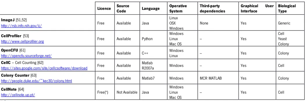
In many studies, such as [49,50] the analysis of CLSM data has been of qualitative rather than quantitative nature and consisted entirely of a visual image inspection. However, this approach is subjective, and not feasible when large quantities of data have to be analysed, which is often necessary to ensure the significance of the outcome of the analyses. For quantitative analysis of images of microorganism aggregates, computer software tools with different functionalities ranging from cell number counting to the classification of colonies morphotypes are currently available. Next, we will present a list (Table 1) several software tools for structural analysis that were reviewed.

(42)

3. Computational tools

25

Table 1: Publicly available image analysis software tools for structural analysis of microorganism aggregates.

In the column “Characteristics” is presented the number of morphology biofilm characteristics described in the previously chapter Software licence Source code Programing language Operative system Third-party dependencies Graphical user interface Biological context Characteristics ImageJ [51,52]

http://rsb.info.nih.gov/ij Free Available Java

Linux OSX Windows

-- Yes Generic Not applicable

CellProfiler [53]

http://www.cellprofiler.org Free Available Python

Windows Linux Mac OS -- Yes Cell Yeast Colony Not applicable PHLIP- Phobia Laser scanning microscopy Imaging

Processor [36]

http://sourceforge.net/projects/phlip/

Free Available Matlab

Linux OSX Windows

Matlab license Yes Biofilms 10

DAIME- digital image analysis in microbial ecology [54]

http://www.microbial-ecology.net/daime/daime

Free Available C++ Windows

Linux -- Yes Biofilms 1

ISA3D - Image Structure Analyzer software [4,55]

www.erc.montana.edu Proprietary

Not

Available Matlab Windows

Matlab license + toolbooxes Biofilms 14 Comstat2 [13,56] http://www.comstat.dk/ Free(*) Not Available Java Linux

Windows ImageJ Yes Biofilms 9

bioImage_L [33]

http://bioimagel.com/ Free(*)

Not

(43)

3. Computational tools

26

3.1 Morphology description software

These programs are very different in terms of their runtime environment, file format acceptance, thresholding procedures, pixel/voxel/object recognition, subject of analysis, volumetric quantification, co-localization analysis, determination of structural parameters, and automation. ImageJ (http://rsb.info.nih.gov/ij/) is a free, open source, and extensive scientific image processing software, developed by Wayne Rasban in 1987, and designed to handle various types of imaging data. Over the years it underwent several changes, keeping however the main ideas: (i) a biological image software that runs on any operative system, with the help of Java Runtime Environment; (ii) has a simple, user-friendly interface, with a single toolbar (see Figure 6); and (iii) extensibility via user-designed macros and plugins. Rasban chose a flexible approach to his software that allows the user to add functionality on their own, but in a manner that would allow sharing with others through macros and plug-ins. Macros are simple custom programming scripts that automate a task inside a large piece of software. The user does not need to have any programming skills to create a macro: in fact, with the help of a “macro record”, it is possible to record any action manually, and thereby create a work flow that one can use repeatedly and share with others. Over 325 macros are currently available at http://rsbweb.nih.gov/ij/macros/. There are also over 500 plug-ins developed by users and available at

http://rsbweb.nih.gov/ij/plugins/index.html. Since these plug-ins were developed to solve specific problems one can expect the continuous increase of this database. The plug-ins are designed to, for instance, count particles or enable the input of more specific instrument file formats — Bio-formats plug-in [51].

(44)

3. Computational tools

27 ImageJ is extremely versatile. It can display, edit, analyse, process, save, and print 8-bit, 16-bit, and 32-bit grayscale and 8-bit and 24-bit colour images. Image formats including TIFF, GIF, JPEG, and BMP can be imported and read as single images or stacks. ImageJ incorporates a number of useful tools for image processing. ImageJ can easily perform background subtraction routines and calculate the area, pixel value statistics, distances, and angles of user-defined selections (with several tools to select a Region of interest). It can also create density histograms and line profile plots. Standard image processing functions such as contrast enhancement, sharpening, smoothing, edge detection, and median filtering are supported as well [51,55,57]. The use of the ImageJ software is reported in [34] for the “Assessment of three-dimensional biofilm structure using an optical microscope”. Hope and collaborators [58], used ImageJ to measure the thickness, and in, Barraud et al. [59] used it to calculate the percentage of the glass surface covered with biofilm.

CellProfiler (http://www.cellprofiler.org) is another good example of a generic yet, extensive image processing software. Due to the pipelining philosophy, it is possible to count colonies and classify them, for example according to the size, automatically identify objects, count them, and record a full spectrum of measurements for each object, including location within the image, size, shape, colour intensity, degree of correlation between colours, texture (smoothness), and number of neighbours [53].

The main purpose of bioImage_L (http://bioimagel.com/) is to allow easy interaction with the implemented image analysis tools, which primarily support input file preparation and output file display, as well as fast data pre-processing and processing, structural calculations of biofilm populations, and graphical displays of individual colour-based subpopulations with graphic outputs of the results. BioImage_L applies an in situ colour segmentation routine that automatically segments the colour image into individual pseudo-channels, and the areas and percentages of each identified colour subpopulation are calculated and presented. The principle of colour segmentation routine relies on the colour addition theory and classifies each pixel of the image into a predefined colour class, resulting in the generation of pseudo channels. Using one of the main advantages of CLSM biofilm images, the z-axis scans, it is possible to reconstruct 3D profiles, and using bioImage_L, calculate the surface and volume distribution of independent subpopulations of cells [4,33].

(45)

3. Computational tools

28 The Open Source software Daime (http://www.microbial-ecology.net/daime/daime) automatically recognizes 2D and 3D objects in single images and confocal image stacks, and offers special functions for quantifying microbial populations. Of note is the quantification of spatial localization patterns of microorganisms in complex samples like biofilms. It also offers many tools for analysing 2D and 3D microscopy datasets of microorganisms stained by FISH with rRNA-targeted probes or other fluorescence labelling techniques. The best quality of Daime is its visualization capabilities, which makes it possible to perform 3D visualization. Other features of this software are biofilm sectioning, spatial arrangement, abundance quantification, image segmentation and object editor [10,14,54].

Comstat (http://www.comstat.dk/) for flow cell biofilm microcolonies, PHLIP (http://sourceforge.net/projects/phlip/) for phototrophic biofilms, ISA-3D (www.erc.montana.edu) for structural as well as DAIME for fluorescence in situ hybridization (FISH) - stained sample analysis are examples of software tools that were especially designed to solve a specific problem in the lab group.

Xavier et al. (2003) developed software to quantify the area of microbial colonization profiles, biovolume, the colonization fraction at the substratum, the average height of microcolonies and interfacial area of morphology of a biofilm for single channel 3D image for CLSM [35]. PHLIP, Phobia Laser scanning microscopy Imaging Processor, extends the functions of the previous version of this software by including a new set of tools to perform quantitative analysis of large amounts of multichannel CLSM data in an automated way, a process necessary to produce statistically meaningful results [36]. PHLIP is also able to quantify ten different biofilm features: biovolume, substratum coverage, area to volume ratio, spatial spreading, mean thickness and roughness, fractal dimension in 2D and co-localization in 2D or 3D [2,33,36,60].

PHLIP was implemented as a MATLAB package and does not require additional toolboxes. The program was developed with flexibility and extensibility in mind, and its functionality can be easily expanded with new features. PHLIP therefore represents a platform for the integration of novel image processing operations without the need to code for import, export, or pre-processing functions. One example of the use of PHILIP to study biofilms is the description of the dynamic spatial and temporal separation of diatoms, bacteria and organic and inorganic matter during the shift from a bacteria-dominated to a diatom-dominated phototrophic biofilm [36].

(46)

3. Computational tools

29 The web-based PHLIP is a program that has a higher level of automation than the ISA and COMSTAT packages, also developed to quantitatively analyse single channel 3D CLSM data of biofilm imaging by determining a set of morphological parameters.

Similarly to PHLIP, ISA3D also has a previous version, called ISA - Image Structure Analyzer software [37]. It was initially developed for the UNIX/Motif environment in C++ with all calculations done in double precision arithmetic, and was able to analyse microscopy images of a biofilm. It was able to compute four areal and three textural parameters: porosity, run length, fractal dimension, diffusion distance and textural entropy, angular second moment inverse difference moment, respectively [2,55]. ISA3D on the other hand, was written using Matlab 7 and can calculate the same parameters as COMSTAT and Xavier et al.’s software. These parameters are: biovolume, volume to surface area ratio, porosity, surface area between biomass and voids, mean thickness, maximum thickness, and roughness coefficient. In addition, with the previous ISA capabilities, the user can now also analyse textural entropy, homogeneity, energy, areal porosity, average horizontal and vertical run lengths, diffusion distance, fractal dimension in two-dimensional image layers, and quantify their distributions with biofilm thickness. ISA3D is menu-controlled, user-friendly, and requires no prior knowledge in programming or image analysis but Matlab need to be equipped with the Image Processing Toolbox.

The measurements available in Comstat are: biovolume, area occupied by bacteria in each layer, thickness distribution and mean thickness, identification and area distribution of microcolonies at the substratum, volumes of microcolonies identified at the substratum, fractal dimension, roughness coefficient, distribution of diffusion distances, average and maximum diffusion distance and surface to volume ratio. All these measurements can be extracted from 3D stack of CLSM biofilm images [13,56].

Examples of analyses which could advantageously be made by Comstat include: (1) analysis of temporal structure development in single-species or community biofilms; (2) comparison of biofilm structures to different organisms or communities under steady-state conditions; (3) determination of the impact of specific mutations on biofilm structure; (4) analysis of the influence of different carbon sources or carbon source concentrations on temporal structure development in single-species or community biofilms; (5) analysis of the influence of antibiotic treatment on the biofilm structure [13].

Mining images of microbial communities for morphological characteristics in a support of clinical decision making

Universidade do Minho

Escola de Engenharia

Ana Catarina de Jesus Domingues

Mining images of microbial communities

for morphological characteristics in a

support of clinical decision making

Universidade do Minho

Dissertação de Mestrado

Escola de Engenharia

Departamento de Informática

Ana Catarina de Jesus Domingues

Mining images of microbial communities

for morphological characteristics in a

support of clinical decision making

Mestrado em Bioinformática

Trabalho realizado sob orientação de

Professora Doutora Anália Lourenço

Professora Doutora Maria Olívia Pereira

Acknowledgements

Resumo

Abstract

Contents

List of Figures

List of Tables

Acronyms

Chapter 1. Introduction

1.1 Context and Motivation

1.2 Thesis contribution

1.3 Dissertation outline

2. Context

Chapter 2. Context

2.1 Biofilms

2. Context

2. Context

2. Context

2. Context

2. Context

2. Context

2. Context

2. Context

2.2 Microscopy - observation techniques

2.2.1 Staining Techniques

2. Context

2. Context

2.2.2 Microscopy

2. Context

2. Context

2.3. Image pre-processing

2. Context

2. Context

2.4 Morphological characteristics

2. Context

2. Context

2. Context

2. Context

3. Computational tools

Chapter 3. Computational tools available for biofilm

analysis

3. Computational tools

3. Computational tools

3.1 Morphology description software

3. Computational tools

3. Computational tools

3. Computational tools