(ISSN online: 2317-6121; print: 1414-5685)
http://br-ie.org/pub/index.php/rbie
Submission: 13/04/2020; 1st round notif.: 13/05/2020; New version: 28/06/2020; 2nd round notif.: 26/08/2020
Camera ready: 19/09/2020; Edition review: 19/09/2020; Available online: 12/10/2020; Published: 12/10/2020
Cite as: Pereira, F. D.; Fonseca, S. C.; Oliveira, E. H. T.; Oliveira, D. B. F.; Cristea, A. I. Cristea & Carvalho, L. S. G. (2020). Deep learning for early performance prediction of introductory programming students: a comparative and explanatory study. Brazilian Journal of Computers in Education (Revista Brasileira de Informática na Educação - RBIE), 28, 723-749. DOI: 10.5753/RBIE.2020.28.0.723
Deep learning for early performance prediction of introductory
programming students: a comparative and explanatory study
Filipe Dwan PereiraFederal University of Roraima [email protected]
Samuel C. Fonseca
Federal University of Amazonas [email protected]
Elaine H. T. Oliveira
Federal University of Amazonas [email protected] David B. F. Oliveira
Federal University of Amazonas [email protected]
Alexandra I. Cristea Durham University
Leandro S. G. Carvalho Federal University of Amazonas [email protected]
Abstract
Introductory programming may be complex for many students. Moreover, there is a high failure and dropout rate in these courses. A potential way to tackle this problem is to predict student performance at an early stage, as it facilitates human-AI collaboration towards prescriptive analytics, where the instructors/monitors will be told how to intervene and support students - where early intervention is crucial. However, the literature states that there is no reliable predictor yet for programming students’ performance, since even large-scale analysis of multiple features have resulted in only limited predictive power. Notice that Deep Learning (DL) can provide high-quality results for huge amount of data and complex problems. In this sense, we employed DL for early prediction of students’ performance using data collected in the very first two weeks from introductory programming courses offered for a total of 2058 students during 6 semesters (longitudinal study). We compared our results with the state-of-the-art, an Evolutionary Algorithm (EA) that automatic creates and optimises machine learning pipelines. Our DL model achieved an average accuracy of 82.5%, which is statistically superior to the model constructed and optimised by the EA (p-value << 0.05 even with Bonferroni correction). In addition, we also adapted the DL model in a stacking ensemble for continuous prediction purposes. As a result, our regression model explained ~62% of the final grade variance. In closing, we also provide results on the interpretation of our regression model to understand the leading factors of success and failure in introductory programming.
724
1 Introduction
Many works have tried to find ways to mitigate the problem of high failure rate (Ihantola et al., 2015; Hellas et al., 2018; Luxton-Reilly et al., 2018; Robins, 2019, Fonseca et al., 2020) in introductory programming courses (CS1). In this sense, researchers (Amra et al., 2017; Costa et al., 2017; Márquez‐Vera et al., 2016; Aguiar & Pereira, 2018; Pereira et al., 2019a; Pereira et al., 2019b; Romero & Ventura, 2019) have argued that early performance prediction is vital. This can facilitate human–AI collaboration towards prescriptive analytics, where the instructors/monitors will be told how to intervene and support students - where early intervention is crucial (Hellas et al. 2018; Alamri et al. 2019; Romero & Ventura, 2019; Pereira et al., 2020a). Furthermore, if the predictive model is interpretable, it can allow understanding the model’s decisions, for a better analysis of which factors can lead to success or failure of learners (Pereira et al., 2019c). With such understanding, we can offer valuable information to instructors and learners. However, Robins (2019) explains that currently there is no reliable predictor yet for programming students’ performance, since even large-scale analysis of multiple features have resulted in only limited predictive power. Still, Ihantola et al. (2015), Quille & Bergin (2018), Hellas et al. (2018) and Robins (2019) state there is a need to advance further in this field.
One potential way to perform such early prediction is by extracting useful information from students’ log-data and use this information as features in machine-learning algorithms (Carter et al., 2019). To illustrate, there are studies which perform prediction using log-data, to represent how students deal with errors (Jadud, 2006; Watson, 2013), deadlines (Robins, 2019; Edwards et al., 2009), attempts and correctness (Castro-Wunsch et al., 2017; Ahadi et al., 2016; Estey & Coady, 2016); static analysis of code (Otero et al., 2016), typing patterns (Leinonen et al., 2016), etc. In this sense, in our previous work (Pereira et al. 2019b), we compiled a set of predictive factors based on the recent literature, which can be used as features in a Machine Learning (ML) model, to predict students’ performance at the very beginning of introductory programming courses. They collected log-data from a home-made online judge, targeted at novice programmers, and employed a method using an evolutionary algorithm, to build and automatically optimise the machine learning pipeline, i.e., without the need of an expert in data science. The evolutionary algorithm explored many combinations of feature selection techniques, machine learning algorithms, combination of hyperparameters and their tuning, to the best ones thus representing a quite competitive technique.
Despite that, the evolutionary algorithm does not explore any deep learning technique for the prediction. However, many researchers (Sadowski et al., 2018; Géron, 2019; Pham et al. 2019, Aljohani et al. 2020) have shown that deep learning can provide high-quality results for huge amount of data and complex problems. With this in mind, it is worth noting that early performance prediction is a complex problem (Robins, 2019). To address it, we use the same number of 2058 students as in Pereira et al.’s (2019b), as this has been shown to be a reasonable amount of data (Hernández-Blanco et al., 2019) to allow for deep learning. Thus, we raised our first research question: (RQ1) Would a deep learning model surpass an evolutionary algorithm for early
prediction of students’ performance?
Moreover, Pereira et al. (2019b) defined the problem of prediction as binary classification, in which a student must earn a final grade of at least 5 (on a scale 0 – 10) in order to pass the course. Robins (2019), Yadin (2013), and Elarde (2016) used the term bimodal outcomes related to CS1 students’ grades, which means that, in general, CS1 classes have mainly two groups: high achievers and failure students. For this, a binary classification make sense, reflecting the bimodal nature of CS1 students’ outcomes. Nonetheless, this approach does not consider properly students in the mid-range. For example, a student with a final grade of 0.1 must be classified the same as one who achieves 4.9 (mid-range student), i.e., both would be classified as failed. On the other hand, students who achieve 4.9 (failed student) must be classified differently than a student who
725
achieves 5.1 (approved student), which is not plausible, as these two students have close grades. As such, we raised a second research question, in order to go a step further than the binary classification: (RQ2) How we can effectively use the same data as for student result classification
in a regression model, to obtain early prediction of the students’ actual final grades?
Additionally, it is critical that education scenarios go a step further than prediction itself and analyse the relevance of features (programming behaviours), with the aim of understanding the major factors that can lead to success or failure for given cohort. In other words, a better understanding of what programming behaviours might negatively or positively influence the students’ grades could lead to a better analysis of which strategies we might use to teach and how our students would like to learn. Thus, we raised our third (and last) research question: (RQ3)
How we can interpret the results of the regression model to better understand what factors can lead to success or failure?
To answer our research questions, we used the same data1 analysed by Pereira et al. (2019b), however, with some new features, a deep learning model, and a new problem definition (continuous prediction). As a result, for classification, our predictive model statistically surpassed (p-value ≪ 0.05) the best model found by Pereira et al.’s (2019b) study. Moreover, our regression model explained 62% of the students’ final grades (r2 = ~0.62, p-value<<0.05). In closing, we interpreted the coefficients of the regression model and discussed pedagogical implication of our early prediction.
Thus, our main contributions with this paper are: a) proposing a new combination of features,
compared to the state of the art baseline, in order to explore potential avenues for enhancing students’ performance; b) showing how a deep learning pipeline can surpass our baseline in the prediction of students’ performance c) performing continuous prediction, instead of only binary classification, with focus not only on prediction performance, but also on the interpretation of the model; d) analysing the effects of the features proposed on the students’ performance.
Briefly, this paper is organised as follows: Section 2 presents our related work, which have similar goals to ours. In Section 3, we show our method, instrument, educational context and data, features described and classified based on a taxonomy, and the explanation on how we build and compare our predictive models. In Section 4, we present, explore and discuss our results. Section 5 shows the limitations of our method. In Section 6, we present our conclusion and future works.
2 Related Work
Research on how to improve the teaching and learning process in introductory programming courses has been a major focus in computing education research (Robins, 2019). For example, there are many relevant works pointing out the advantages of using e-learning systems, such as
online judges (Wasik et al., 2018). Some propose methods of exploring the large-scale data that
come from the interaction of students with these systems (Luxton-Reilly et al., 2018; Wasik et al., 2018). This kind of data collection enables a data-driven analysis of student behaviours (Ihantola et al., 2015, Pereira et al. 2018, Aguiar & Pereira, 2018; Carter et al., 2019), important to encapsulate the learners’ progress during the programming courses (Watson et al., 2013; Pereira et al., 2020a). In this context, early performance prediction is gaining increasing attention, as it creates the possibilities to leverage the educational outcomes via early interventions (Hellas et al. 2018; Romero & Ventura, 2019; Pereira et al., 2020a). In general, researchers in this field investigate features that can be used in machine learning algorithms to make predictions (Hellas et al., 2018). This section presents some relevant work that can contribute in the search of solutions to the problem of early prediction of CS1 student’s performance, using data collected from
726
learning systems employed in programming classes. Moreover, we draw parallels to our work to show both the need for it and its additional contributions.
Many works (Jadud, 2006; Watson et al., 2013; Ahadi et al., 2016; Estey & Coady, 2016; Leinonen et al., 2016; Márquez‐Vera, 2016; Castro-Wunsch et al., 2017; Costa et al. 2017; Amra & Maghari, 2017; Pereira et al. 2019a; Pereira et al. 2019b) have been collecting fine-grained data in the context of programming classes, to model students’ behaviour and to quantify aspects of students’ performance. All these studies have in common that they analyse the data-driven student behaviours, extract useful information, and use them as features in machine learning and inferential statistics techniques, with the goal of predicting the CS1 students’ performance at an early stage in the course.
Costa et al. (2017) conducted an important work in predicting students’ outcomes, comparing different machine learning algorithms and the impact of data pre-processing and fine-tuning of hyperparameters. The authors analysed data from 262 distance education students and 161 on-campus learners. They used demographic features, such as age, gender, civil status, and other data-driven features, like number of accesses to the system and participation in discussion forums. Their best prediction results have an f-score of 82% for on-campus students and an f-score of 80% for distance education ones, both results using data from the first two weeks of the course. Although the outcomes of this work are promising, their database is small. Moreover, their use of demographic data is static in nature and, hence, fails to encapsulate changes in students’ learning progress during the course. Still, their results missed out on continuous prediction (regression). They also did not explain their machine learning model’s decisions. In this paper, we also use their early, first-two-weeks-based prediction idea. However, we present a different approach, using non-static, data-driven features for predicting student’s grades both for discrete and
continuous outcome. Moreover, we explore the use of deep learning, instead of only shallow
models and we interpret the model’s results.
In a pioneering and highly cited study, Jadud (2006) conducted a data-driven analysis to propose an algorithm called Error Quotient (EQ), which uses snapshots of compilation, to quantify the errors from the students, while they are programming. In essence, the EQ algorithm received as input a pair of compilation events and assigned to them a penalty, if errors were found. The penalty could vary; for example, if the error of both compilation events were the same, then the penalty would be greater, as the student would be showing the same misunderstandings repeatedly. Watson et al. (2013) extended EQ with an algorithm computing the watWinScore, which scores compilation pairs, by additionally taking into account the problem resolution time. However, the results of these algorithms were modest in predicting students’ outcomes. The algorithm proposed by Watson et al. (2013) obtained an average accuracy of 68.8% during the course, whereas the EQ results had an average accuracy of 55.8%, both for performance prediction in an experiment reported by Watson et al. (2013) with 45 programming students. In addition, for a regression task, the EQ explained ~30% (r2 = 0.3005) of the students’ grades, whilst
watWinScore explained somewhat more, but still only ~42% (r2 = 0.4249), both using data from
the entire course. Using data from the beginning of the course (first 3 weeks), EQ and
watWinScore had a poorly explained variance ranging from 5% to 10% (r2 = [0.5 – 0.1]). Despite
the poor results for early prediction, they provided some interesting ideas, useful to explore in another education context. Thus, we considered using the EQ and watWinScore together, as features in a machine learning model, to investigate their predictive power in conjunction.
Leinonen et al. (2016) used Machine Learning models to detect students with prior programming experience and to infer which students will pass or fail in CS1 classes. In order to do so, they used features based on typing patterns (e.g., number of pairs of alphabetic or numeric characters) and keystroke latency. For the problem of detecting whether the students would pass or not, they also achieved a modest accuracy of 65.8%, using data from 226 students in their first
727
two weeks of course. Similar to EQ and watWinScore, more studies were considered to be required to be conducted, to check whether some combination of the features presented by Leinonen et al. (2016), together with others, would achieve higher outcomes.
Castro-Wunsch et al. (2017) adopted deep learning and traditional ML models to identify students (n=897) in need of assistance. The authors found that the number of attempts for each code exercise and the proportion of test cases accepted (correctness) in problems from online judges are effective predictors to be used as features in machine learning models. As a result, they achieved the best accuracy of 71.81%, using data from the fourth week of the course. Still, Castro-Wunsch et al. (2017) suggested in their conclusions that deep learning would likely achieve better results, with new combination of features and more data. Following this, and using similar features as Castro-Wunsch et al. (2017), Estey & Coady (2016) revealed that students at risk not only have fewer submission attempts, but also a lower compilation frequency, and different patterns in relation to the repeated consumption of hints generated in an online environment. Using data from 652 students for early prediction (first two weeks), Estey & Coady (2016) achieved an accuracy for the failing students of 30%. In brief, Castro-Wunsch et al. (2017) and Estey & Coady (2016) demonstrated the predictive power of simple metrics (e.g., attempts and correctness), however their results were still modest. As such, there is a need of more improvements and new experiments with other features.
In an exploratory study, Auvinen (2015) analysed deeply the programming behaviours of 1777 students in an online judge and found that studying close to the deadline and trial and error behaviour is related to poor performance. Kazerouni et al. (2017) tracked and assessed procrastination behaviours and the amount of change of 370 students while solving programming problems. To check the positive and negative effect of such behaviours, they interviewed the students. As a result, they confirmed what Auvinen (2015) has found that procrastination behaviours can be dangerous for programming students. Following, Otero et al. (2016) analysed code metrics of programming students’ codes, such as number of lines, number of conditions and so forth. As a result, the authors suggested that these code metrics were related to the student’s performance. Again, all these works are relevant, however there is a need to understand their predictive power together in machine learning models, using data collected from different educational institutions.
In this sense, in an effort to compile these data-driven programming behaviours (features) exposed previously in this section, Pereira et al. (2019b) have used some adaptations of code metrics proposed by Jadud (2006), Watson et al. (2013), Ahadi et al. (2015), Estey & Coady (2016), Ahadi et al. (2016), Leinonen et al. (2016), Otero et al. (2016), Castro-Wunsch et al. (2017), Pereira et al. (2019a) as features in ML models. As a result, Pereira et al. (2019b) achieved an accuracy between 71% and 82% by using a traditional ML model optimised by an evolutionary algorithm. To train and validate the model, Pereira et al. (2019b) used data collected from 2058 learners in the first two weeks of introductory programming courses.
Meanwhile, deep learning revolutionised the field of machine learning, by obtaining state-of-the-art results (Miikkulainen et al., 2019). Many areas have benefited from applying deep learning, and education is no exception (Hernández-Blanco et al., 2019). Moreover, as stated by Robins (2019) in a recent book, predicting programming students’ performance is a complex problem. Géron (2019) explains that deep learning is suitable for large amounts of data (as for the Pereira et al. dataset) and complex problems (such as the early prediction performance of programming students).
In addition, Ihantola et al. (2015), Quille & Bergin (2018), Hellas et al. (2018) and Robins (2019) claimed that more studies need to be replicated and new methods need to be proposed in order to advance in this field. In this sense, we reproduce here the relevant state of the art study
728
from Pereira et al. (2019b), and extend it with deep learning, as well as additional features, as a move towards advancing in predicting introductory programming students’ performance.
3 Method
In this work, we validate and compare machine learning pipelines with the goal of: i) estimating whether students will pass or not in a CS1 course using classification models; ii) predicting the students’ final grades using regression models; and iii) interpreting what programming behaviours are leading factors for success and failure. To do so, we used data collected from a home-made online judge that will be described next.
3.1 Instrument
We used an online judge called CodeBench, developed from scratch by one of the authors for automatic evaluation of students’ solutions. For evaluating students’ code, CodeBench uses test cases, to check if a student’s code output matches with the expected output (Wasik et al., 2018; Pereira et al., 2020b). Following are the definitions of Test Cases, Solution, and Correctness
Analysis.
Definition 1 (Test Case): C = (I, O) is a tuple, where I is a set of inputs ii and O is a set of expected outputs oi for I, where i = 1...n.
Definition 2 (Solution): given an output oi and an input ii there is a family of functions F = {f: I ⇒ 0 | ii ⇒ oi}, which represents a set of programs (solutions) that satisfy the correctness conditions of a given problem q.
Definition 3 (Analysis of correctness): given a function f' submitted by a student, this will satisfy the correctness conditions of the problem q, if f' ∈ F.
It is worth noting that students do not have access to the test cases that will be used to evaluate their codes. After analysing the correctness of the student’s code, the CodeBench returns to the student a verdict whether the code is correct or not, with some qualifications2. In the case of CodeBench, a typical interaction between students and the online judge are:
the student writes a solution in the Integrated Development Environment (IDE) embedded in CodeBench;
the student runs and tests the code in the IDE using the programming language compiler; the student submits the code to the evaluation of CodeBench;
CodeBench automatically returns a feedback to the student, telling whether the code is correct or not. If it is wrong, CodeBench also returns a percentage of successful test-cases. The students are allowed to submit their solution as many times as they want, with no penalty.
3.2 Data
We used the data extracted from students’ interactions with CodeBench during their attempts to solve the programming problems, as explained in the previous subsection. Each assignment has 10 programming problems. These activities are followed by an exam, conducted in the same web-based system. There were 2 programming problems in each exam. The problems from the exams were on the same topics as the assignment beforehand. The exams were shorter because they were
2 When the student submission is incorrect, there are many ways of generating feedback, such as compilation error,
729
face-to-face in a lab. In this paper and in our baseline, we call each pair formed of an assignment and an exam a 'session'. In total, 7 sessions were held throughout the course, lasting a little over 2 weeks each.
For the training of machine learning algorithms, we use only the data from the first session (first
two weeks), since the purpose of this study is to investigate early predictors. The content of the
seven sessions were: variables and sequential structure (S1), conditionals (S2), nested conditionals (S3), ‘while’ repetition structures (S4), vectors and strings (S5), ‘for’ repetition structures (S6), and bi-dimensional matrix (S7). Thus, the sessions were structured so that problems became gradually harder.
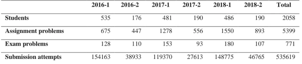
In total, 2058 students solved programming problems from the assignments and exams, all using the Python programming language during 6 semesters (2016-2018) in the Federal University of Amazonas. An unlimited number of submission attempts were allowed in the exams and in the proposed problems from the assignments, as long as they met the deadline. Table 1 shows some descriptive statistics of the data we collected during six consecutive terms [2016-2018]. In total, we analysed data from 5399 programming problems, 771 problems from exams, and 535,619 submission attempts from those learners.
Table 1: Number of instances in CodeBench’s data set (by term)
2016-1 2016-2 2017-1 2017-2 2018-1 2018-2 Total
Students 535 176 481 190 486 190 2058
Assignment problems 675 447 1278 556 1550 893 5399
Exam problems 128 110 153 93 180 107 771
Submission attempts 154163 38933 119370 27613 148775 46765 535619
For a better understanding of the data we used, Figure 1 presents a simple example of the log-data, from which we extracted useful information, to construct a programming profile for each student. This data was collected directly from the IDE, where students spend the majority part of their time on problem-solving. Thus, this fine-grained log-data annotated with events of tests, submissions, executions, keystrokes, provides us a broad spectrum of programming behaviours. To illustrate, Figure 1 shows an excerpt from this fine-grained log, where one can see that a given student clicked on the IDE (focus event – line 1) at 08:34am on the 27/05/2016 and ~1 millisecond later, he/she pressed the key “p” (change event – line 2). Subsequently, he/she typed “rint()”, completing the Python command “print”.
Figure 1: Example of logs collected when the learner was writing a “print” command (Pereira et al., 2020a).
Table 2: Features (programming behaviour) used on our programming profile
Feature (programming behaviour)
Description Type
procrastination Time between first code edit and programming assignment deadline, multiplied by -1 (Carter et al., 2019; Edwards et al., 2009)
Count
amountOfChange In a pair of consecutive submissions to the same problem, amountOfChange refers to the number of lines added or changed from the first to the last code submitted (Carter et al., 2019; Edwards et al., 2009).
730
eventActivity A binary value, which equals 0 when a student solves a problem within less than a number3 of log lines (events), or 1 otherwise.
Algo
attempts Average number of submission attempts by students (regardless whether correct or not) (Ahadi et al., 2016).
Math
lloc Average number of logical lines for each submitted code (Otero et al., 2016). Imports, comments, and blank lines were not counted.
Math
systemAccess Number of student logins up to the end of the second week (adapted from Pereira et al. (2019b)).
Count
firstExamGrade Student’s grade in the first exam, taken in the second week of the course (Pereira et al., 2019b).
Count
events4 Number of log lines on attempting to solve problems. To illustrate, each time the
student presses a button in the embedded IDE, this event is stored as a line in a log file (adapted from Leinonen et al. (2016) and Castro-Wunsch et al. (2017).
Count
correctness Number of problems correctly solved from programming assignments before the first exam (Pereira et al., 2019b).
Count
correctnessCodeAct Represents the same as correctness, but in this case, we consider ‘correct’ only student’s solutions with more than 50 events. To illustrate, if a student submits a correct solution by copying and pasting (only 1 event), for this problem it will be assigned 0 to the feature correctnessCodeAct, however for the feature correctness will be assigned 1 (Pereira et al., 2019b).
Algo
copyPaste Proportion between pasted characters (‘ctrl+V’) and characters typed (Pereira et al., 2019b).
Math
syntaxError Ratio between the number of submissions with syntax error5 and the number of
attempts (Estey & Coady, 2016; Pereira et al., 2019b).
Math
ideUsage Total time (in minutes) spent by students solving problems in the embedded IDE (it removes inactive time – more than 5 minutes without typing) -Adapted from Pereira et al. (2019b).
Algo
keystrokeLatency Keystroke average latency of the students when typing in the embedded IDE (we also removed downtime) – adapted from Leinonen et al. (2016).
Algo
errorQuotient Compute a score based on the number of code errors and repeated errors (Jadud, 2006) - more explanation in related work section
Algo
watWinScore An extension of errorQuotient which considers the problem-solving time (Watson et al., 2013) - more explanation in related work section
Algo
deleteAvg average of deleted characters for each problem (Pereira et al., 2019b) Count
countVar Number of variables in the source code (Carter et al., 2019) Count
3.3 Student Programming Profile
A 'programming profile' for each student in the first session (S1) was constructed by using 18 code features (programming behaviours) which represented metrics proposed by state-of-the-art studies. This 'student programming profile' was then digitally represented as a feature matrix, i.e., allocating each student a row and each feature a column. The features and corresponding description are listed on Table 2, and sources are given. Furthermore, Table 2 shows a column Type, based on Carter et al. (2019) taxonomy, where Count means programming behaviours extracted using only the frequency of events on the log-data; Math means the need of a
3
One standard deviation minus the median of the numbers of events for a problem
4 Castro-Wunsch et al. (2017) called this feature 'number of steps'. However, unlike them, we averaged it. 5
731
mathematical formula to extract the useful information, whilst Algo means the use of an algorithm to perform such extraction.
It is worth noting that with exception of procrastination, amountOfChange and
eventActivity, all the features presented on Table 2 were used by our baseline, Pereira et al.
(2019b), and Pereira et al. (2020), which were chosen after a process of pairwise correlation analysis to avoid multicollinearity.
3.4 Cleaning the features and dealing with imbalanced dataset
First, for classification, we normalise our features using MinMax (equation 1) to produce maximum absolute value of each feature scaled in unit size. We used this scaling technique due to its robustness to features with small standard deviation as ours and because it preserves zero entries. Moreover, such scaling technique is important for neural networks because if a feature has a variance that is orders of magnitude larger than others, the estimator might be unable to learn from other features correctly as expected (Géron, 2019; Pedregosa et. al, 2011).
𝑋𝑋𝑠𝑠𝑠𝑠𝑠𝑠 =𝑚𝑚𝑚𝑚𝑚𝑚(𝑋𝑋) − 𝑚𝑚𝑚𝑚𝑚𝑚 (𝑋𝑋)𝑋𝑋 − 𝑚𝑚𝑚𝑚𝑚𝑚(𝑋𝑋) (1) Moreover, the data generated by students that did not attend the course were removed from this analysis, since they did not have any interaction with the online judge. In addition, the database is very slightly unbalanced, since, unlike in other educational environments there are somewhat more students who passed (~56.7%) than failed (~43.3%). As we are dealing with features extracted from a very fine-grained log-data collected from students’ interactions with an online system, some packets of data may be lost before reaching the server side. To illustrate, if a student loses internet connection while solving a problem on the IDE, then his/her logs will not be sent properly to the server. Still, students can start the course with a desirable behaviour, engaged, solving many problems from the assignments and performing well on the first exam, but change throughout the course, possibly due to external factors, ending with a low grade (and vice-versa). As such, our database might have some outliers. Thus, aiming to decrease the biases of the classifiers due to the unbalanced nature of the database and the presence of outliers, we used a statistical technique called Tomek Links (Tomek, 1976) to remove noise. When a Tomek’s link is formed on unbalanced datasets (as ours), Batista (2002) recommended removing one instance from the majority class, in order to decrease the unbalance of the database, while also removing noise. Using this approach, we removed 100 instances from the majority class (students who passed) that form Tomek’s links on our database.
Notice that a Tomek’s link (L_T) is defined between two samples xi and xj of different classes c1 and c2, respectively, for any sample y (equation 2), where d(.) is the Euclidean distance between the two samples. In other words, a Tomek’s link is represented by two samples from different classes that are the nearest neighbours of each other, which might confuse the ML model, when creating the decision boundaries to separate the instances of each class (Batista, 2002).
L_T = d(x1, x2) < d(x1,y) and d(x1, x2) < d(x2,y) (2) To further deal with our imbalanced dataset, we divided the data into homogeneous subgroups called stratum (stratified sampling), so that the right number of instances is sampled from each stratum in order to keep the same class proportion in the training and validation sets (Géron, 2019). To do so, we used the library StratifiedKFold from scikit-learn (Pedregosa et al., 2011), using a total of 10 folds.
For regression, we simply divided the data into training (70%) and testing (30%) as the outcome is continuous and, hence, there is no problem of unbalancing. Moreover, instead of
732
in terms of standard deviation, making it easy to interpret the coefficients and features values of the regression model.
𝑧𝑧𝑖𝑖=𝑚𝑚σ(𝑚𝑚𝑖𝑖)𝑖𝑖− 𝑚𝑚̅ (3)
3.5 Prediction and Validation
First, it is important to explain how the task of classification is performed, when the target is a continuous variable. We will employ the same approach used by the state of the art represented by our baseline, Pereira et al. (2019b), which represented the problem as a binary classification, where students that achieve a final grade greater or equal to 5 are represented as the class ‘passed’, the rest being ‘failed’. In Pereira et al. (2019b), the authors justified the grade 5, by arguing that this is the threshold used by the university where they collected the data from.
In terms of machine learning pipeline, our baseline, Pereira et al. (2019b), explained that the model found by the evolutionary algorithm was a regularised Random Forest (RF) with 100 constituent decision trees that considers 30% of the features when splitting the constituent decision trees using bootstrap for resampling. Moreover, the trees must have at least 8 instances to create a new branch. To perform the classification, the RF used hard-voting.
To validate our hypotheses that a deep learning model will outperform the model found by Pereira et al (2019b), we adopted the popular and widely used Multilayer Perceptron (MLP). We use MLP, as this is one of the most effective neural network techniques for modelling and prediction (Pham et al. 2019). In addition, many researches (Sadowski et al., 2018, Pham et al. 2019) have claimed that MLP can be effectively employed for modelling nonlinear and complex processes of the real world, and education is not an exception (Hernández-Blanco et al., 2019). In brief, MLP is a neural network fully connected that comprises an input layer followed by one or more hidden layers, and a final output layer. MLP is a feed forward NN as the data flows only from the input to the output. MLP is considered a deep learning model as many authors use this term whenever neural network is involved (Géron, 2019), even for shallow NN.
In general, deep learning models are suitable for huge amount of data and complex problems (Sadowski et al., 2018; Géron, 2019; Pham et al. 2019). Here, we are tackling a complex problem (Robins, 2019; Pereira et al. 2019), however with not that much data. In this scenario, a highly deep MLP will likely perform well on the training, but not on the testing set (overfitting). As such, we configured our MLP with only two hidden dense6 layers. Each dense layer has 64 nodes and we use the state-of-the-art Rectified Linear Unit function (RELU) as activation function. We initialised the weights and biases of our NN randomly, following a normal distribution as widely recommended (Géron, 2019). As a way of regularising our NN, we added the widely used dropout technique (Hinton et al., 2012; Srivastava et al., 2014) followed by each hidden dense layer. We configured the dropout with p=0.57, which means that 50% of the neurons of a hidden layer are ignored during training. Still, we used adaptive moment estimation (adam) technique (Kingma & Ba, 2014) for optimisation of the gradient descent, as this method tends to accelerate the convergence of the model and reduces the fast decay of the learning rates (Géron, 2019). In addition, we used the popular binary cross entropy as loss function for our classification problem. The output layer has two nodes, one for each class, and uses the sigmoid activation function, which gives a probability of a student passing or failing.
Moreover, a continuous estimation of students’ grades can be more useful for instructors, as it is more detailed and thus more powerful and information rich than a binary classification
6 It is called a dense layer when all the neurons in a layer are connected to every neuron in the previous layer (fully
connected layer) (Géron, 2019).
733
(passed or failed). In this sense, we go a step further by adopting, besides classification, a regression model, to perform continuous estimation. To do so, we adapted the ideas behind stacking ensemble (Wolpert, 1992). We configured the stacking ensemble using the outcome (predicted probabilities) from the MLP model as input on a meta-classifier (blender). In other words, as we performed 10-fold stratified cross-validation for the classification problem with our DL model, we have a probability prediction for each student based on the sigmoid activation function, which is estimated on each test fold of the cross validation. As such, these probabilities as one of the features (dlProbs) in our Ridge Regression model. Thus, we used this ‘meta-feature’ concatenated with the features from the programming profile (presented on Table 2) and used as input on an easily interpretable Ridge Regression algorithm, that worked as a meta-classifier (blender) on the stacking ensemble. This allows us to have the predictive power of our deep learning model (by using its outcome) along with the interpretability power of a Ridge regression linear model, which is important to understand the early programming behaviours that might be positive or negative in terms of success and failure in CS1 courses. We opted for Ridge Regression, as this regularised version of a linear regression is a good default in cases where we suspect that almost all features will likely be useful (Géron, 2019).
As extra information, we state that we also performed tests with other machine learning algorithms in the regression task (RandomForest, Extra Trees, XGboost and others), including with optimisation of hyperparameters; however, the results were not significantly superior to those found with our linear model of regression. Therefore, we chose to use Ridge Regression, which gives us, in addition to the predictive power, an easy interpretation of the confidence intervals of the regression coefficients.
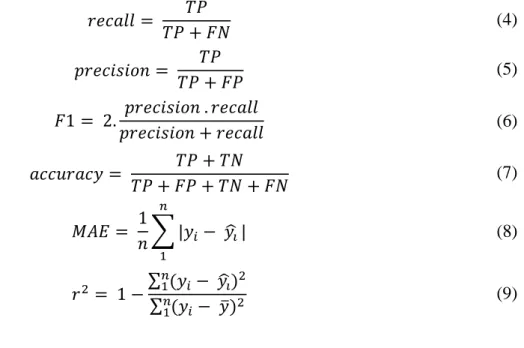
For classification, we compared both models, using the following statistical metrics suitable for unbalanced dataset such as ours: recall (equation 4), precision (equation 5), F1-score (equation 6), and accuracy (equation 7), where TP stands for true positive, TN stands for true negative, FP stands for false positive, and FN stands for false negative. For regression, we used the widely recommended (Montgomery, 2012) MAE (equation 8) and the coefficient of determination r2 (equation 9), where n is the number of samples, 𝑦𝑦𝚤𝚤� is the predicted value of the
734 𝑟𝑟𝑟𝑟𝑟𝑟𝑚𝑚𝑟𝑟𝑟𝑟 = 𝑇𝑇𝑇𝑇 + 𝐹𝐹𝐹𝐹𝑇𝑇𝑇𝑇 (4) 𝑝𝑝𝑟𝑟𝑟𝑟𝑟𝑟𝑚𝑚𝑝𝑝𝑚𝑚𝑝𝑝𝑚𝑚 = 𝑇𝑇𝑇𝑇 + 𝐹𝐹𝑇𝑇𝑇𝑇𝑇𝑇 (5) 𝐹𝐹1 = 2.𝑝𝑝𝑟𝑟𝑟𝑟𝑟𝑟𝑚𝑚𝑝𝑝𝑚𝑚𝑝𝑝𝑚𝑚 + 𝑟𝑟𝑟𝑟𝑟𝑟𝑚𝑚𝑟𝑟𝑟𝑟𝑝𝑝𝑟𝑟𝑟𝑟𝑟𝑟𝑚𝑚𝑝𝑝𝑚𝑚𝑝𝑝𝑚𝑚 . 𝑟𝑟𝑟𝑟𝑟𝑟𝑚𝑚𝑟𝑟𝑟𝑟 (6) 𝑚𝑚𝑟𝑟𝑟𝑟𝑎𝑎𝑟𝑟𝑚𝑚𝑟𝑟𝑦𝑦 = 𝑇𝑇𝑇𝑇 + 𝐹𝐹𝑇𝑇 + 𝑇𝑇𝐹𝐹 + 𝐹𝐹𝐹𝐹𝑇𝑇𝑇𝑇 + 𝑇𝑇𝐹𝐹 (7) 𝑀𝑀𝑀𝑀𝑀𝑀 = 1𝑚𝑚� |𝑦𝑦𝑖𝑖− 𝑦𝑦𝚤𝚤� 𝑛𝑛 1 | (8) 𝑟𝑟2 = 1 −∑ (𝑦𝑦𝑖𝑖𝑛𝑛1 − 𝑦𝑦𝚤𝚤�)2 ∑ (𝑦𝑦𝑖𝑖𝑛𝑛 − 𝑦𝑦� 1 )2 (9)
4 Results and Discussion
We organised the results in four subsections, in order to answer our three research questions. In subsection 4.1, we compare our deep learning model with the best previous model found (Pereira et al., 2019b) using an evolutionary algorithm, answering RQ1. In section 4.2, we show the results of our regression model, in order to respond to RQ2. Furthermore, in education, it is also important to understand which behaviours mostly affect student performance. As such, answering RQ3, in subsection 4.3, we analyse how each feature affected the regression model outcome in a move towards understanding each positive and negative programming behaviour from the students’ programming profile. Finally, in subsection 4.4 we discuss the pedagogical implication of early prediction in introductory programming courses.
4.1 Deep Learning versus Evolutionary Algorithm
First, we check whether the features listed in Table 2 are relevant to distinguish programming behaviours from students who passed and failed and, hence, whether they would be useful as features for the ML model and for our explanation of the model decision. For this, we first applied the non-parametric Mann-Whitney U test to compare the features of students who passed or failed. Results indicate a statistical difference (even with Bonferroni correction: p ≪ 0.05/18) between all features. Hence, we opted not to perform feature selection and use all features as input to construct our predictive model. Another reason for not performing feature selection is that it is intrinsic to deep learning models to automatically extract the best.
Given that, in this subsection we answer our first research question (RQ1): ‘Would a deep
learning model surpass an evolutionary algorithm for early prediction of students’ performance?’
To answer this question, we ran the model proposed by Pereira et al. (2019b) using the features presented in their paper, as well as additional features (as explained in subsection 3.3), and used their classification settings (constructed and optimised by an evolutionary algorithm), as presented by them. Subsequently, we compared the results with our predictive model proposed in the current paper (both predicting models are explained in subsection 3.5). For each predictive model, we ran the stratified cross-validation 20 times with 10 folds, varying the seed over a range from 1 to 20, in order to shuffle the database in different ways and, hence, explore the range of possible outcomes. Hence, we obtained 200 results for each metric (10 x 20), one outcome for each fold.
Table 3 shows the descriptive statistics of each model outcome, in which Random Forest (RF) depicts the model constructed and optimised by the evolutionary algorithm, trained with the
735
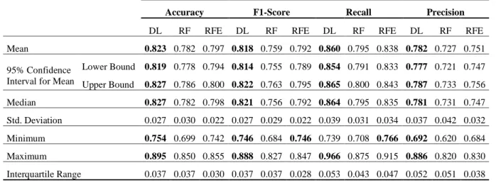
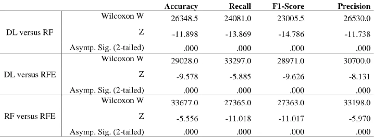
features used by Pereira et al. (2019b), whereas Random Forest Extended (RFE) is the same model, but trained with our extended features (presented in Table 2). Our deep learning model achieved an accuracy ranging from ~81.9% to ~82.7% (C.L. 95%) using data from the first two weeks of the course for training, whereas the RF model found by our baseline achieved an accuracy ranging from ~77.8% to 78.6% (C.L. 95%). To check for statistical significance, in Table 4, we define null hypotheses and, in Table 5, we show the pairwise Wilcoxon test results to check these null hypotheses. Indeed, Table 5 shows that our model (DL) statistically surpasses our baseline (RF), even after Bonferroni correction (p-value ≪ 0.05/4) in all model evaluation metrics (accuracy, F1-score, precision and recall), which shows that we can better recognise (higher recall) students who pass and fail with a higher precision. Thus, we can refute the null hypotheses
H01, H04, H07, H010.
Table 3: Descriptive Statistics of the predictive models outcomes (higher results are bolded).
Accuracy F1-Score Recall Precision DL RF RFE DL RF RFE DL RF RFE DL RF RFE Mean 0.823 0.782 0.797 0.818 0.759 0.792 0.860 0.795 0.838 0.782 0.727 0.751 95% Confidence
Interval for Mean
Lower Bound 0.819 0.778 0.794 0.814 0.755 0.789 0.854 0.791 0.833 0.777 0.721 0.747 Upper Bound 0.827 0.786 0.800 0.822 0.763 0.795 0.865 0.800 0.843 0.787 0.733 0.756 Median 0.827 0.782 0.798 0.821 0.756 0.792 0.864 0.795 0.835 0.781 0.731 0.747 Std. Deviation 0.027 0.030 0.022 0.027 0.029 0.022 0.039 0.031 0.034 0.037 0.042 0.032 Minimum 0.754 0.699 0.742 0.746 0.684 0.746 0.739 0.708 0.766 0.692 0.620 0.684 Maximum 0.895 0.850 0.855 0.888 0.827 0.847 0.966 0.875 0.915 0.886 0.820 0.830 Interquartile Range 0.037 0.037 0.030 0.037 0.037 0.028 0.053 0.043 0.047 0.052 0.051 0.038
DL stands for Deep Learning, RF stands for Random Forest, and RFE stands for Random Forest with the Extended features Table 4: Hypothesis Summary.
H01 The distribution of Accuracy is the same between the models DL and RF. H02 The distribution of Accuracy is the same between the models DL and RFE. H03 The distribution of Accuracy is the same between the models RF and RFE. H04 The distribution of F1-score is the same between the models DL and RF. H05 The distribution of F1-score is the same between the models DL and RFE. H06 The distribution of F1-score is the same between the models RF and RFE. H07 The distribution of Recall is the same between the models DL and RF. H08 The distribution of Recall is the same between the models DL and RFE. H09 The distribution of Recall is the same between the models RF and RFE. H010 The distribution of Precision is the same between the models DL and RF. H011 The distribution of Precision is the same between the models DL and RFE. H012 The distribution of Precision is the same between the models RF and RFE.
Moreover, we further compared our model with our baseline in another setting, with our new combination of features presented in Table 2. Remember, we have added 3 features (procrastination, amountOfChange and eventActivity) to the features presented by Pereira et al. (2019b). Thus, using this new combination of features and the same data, we ran the model found by the evolutionary algorithm 200 times for each metric. Again, our deep learning model surpasses our baseline (RFE, in this case), even with Bonferroni corrections (p-value ≪ 0.05/4) for all model evaluation metrics. Hence, we can refute the null hypothesis H02, H05, H08, H011. In addition, we can observe in Table 4 that RFE statistically surpasses RF, what suggests that our extended
736
features play an important role for the classification process and, hence, we can refute the null hypothesis H03, H06, H09, H012.
Table 5: Pairwise Wilcoxon test to compare the predictive models.
Accuracy Recall F1-Score Precision
DL versus RF
Wilcoxon W 26348.5 24081.0 23005.5 26530.0 Z -11.898 -13.869 -14.786 -11.738
Asymp. Sig. (2-tailed) .000 .000 .000 .000
DL versus RFE
Wilcoxon W 29028.0 33297.0 28971.0 30700.0
Z -9.578 -5.885 -9.626 -8.131
Asymp. Sig. (2-tailed) .000 .000 .000 .000
RF versus RFE
Wilcoxon W 33677.0 27365.0 27363.0 33198.0
Z -5.556 -11.018 -11.017 -5.970
Asymp. Sig. (2-tailed) .000 .000 .000 .000
Therefore, we now will further explore the results of our deep learning model, focussing on our new combination of features. In Figure 2a, we show the precision/recall curve of our model for different thresholds, whilst in Figure 2b we show the ROC curves, i.e., the false positive rate (x axis) and true positive rate (y axis) also for different thresholds, where class 0 depicts the students who fail and class 1 represents the students who passed. Before the explanation about Figure 2 (a and b), it is worth illustrating what means threshold in the context of these figures. In a binary classification task as ours, the DL algorithm uses probability to classify a student as passed or failed. Thus, to perform the classification, the model uses a standard threshold of 0.5 (50%). Therefore, if the model estimates that the probability of a student passing is 60% and the threshold is equal to 50%, then the student will be classified as passed. On the other hand, the same student would be classified as failed if the threshold is equal to 70%. Note that increasing the threshold increases the confidence level to classify a sample as passed, however the algorithm's hit rate decreases, as it tends to estimate an observation as pass, only when it has a higher level of confidence.
Given that, from a visual inspection of Figure 2, it is possible to see that our model indeed performed well on both classes. With regards to the precision/recall curve, we achieved an area under the curve of 0.854 for students who passed and ~0.92 for learners who failed. Still, with regards to the ROC curves, we achieved an area under the curve of 0.90 in both classes. This shows that our model segregated students who passed and failed, even when the threshold was different from the central value (0.5). This can be seen by analysing the continuous lines (green and black) of Figure 2 (left and right) that are close together, sometimes overlapping.
737
Figure 2: Precision and recall curve (left) and ROC curve (right) of students who passed (class 1) and students who failed (class 0). Micro-average takes into consideration the class proportion of students who passed and failed, whereas macro-average threat
each class independently. 4.2 Regression Analysis
In this subsection we answer our second research question (RQ2): ‘How we can effectively use
the same data as for student result classification in a regression model, to obtain early prediction of the students’ actual final grades?’
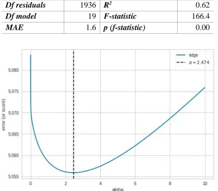
As we are using a linear model with regularisation, Ridge Regression, we first adjust the alpha value, which controls the amount of regularisation, i.e., the higher the alpha, the less complex (and higher bias) the model, whereas the lower the alpha, the more complex (and higher variance) the model. Notice that too complex models can lead to overfitting, whilst a too simple model can cause underfitting. Thus, we tested different values of alpha to find a balance between this bias-variance trade-off, as can be seen in Figure 3. As a result, the best value found is alpha=2.474 (see the vertical dotted line). Using this alpha, we achieved a coefficient of determination (r2) of ~0.62 (see Table 6). Thus, overall, our model can explain 62% (r2~=0.62) of the variance on students’ final grades, by using a relatively high degree of freedom for the residuals (Df residuals) and a low degree of freedom for the model (Df model). This is important in linear regression, as
r2 only increases when the Df model (number of features + 1) increases (Montgomery et al., 2012). Indeed, the predictions of our regression model is statistically significant (p-value < 0.05 and
f-statistics = 166.4).
Table 6: Regression Results. Df stands for degrees of freedom, MAE stands for mean absolute error.
Df residuals 1936 R2 0.62
Df model 19 F-statistic 166.4
MAE 1.6 p (f-statistic) 0.00
Figure 3: Choosing the optimal alpha for our Ridge Regression Model. We use as error measure the Mean Squared Error (y axis) as this statistic metric gives a higher penalty to errors than Mean Absolute Error and Coefficient of Determination.
In addition, for a better understanding of our regression’s performance, we evaluated our MAE, which is ~1.6 [+/- 0.11, CL of 95%] (Table 6), what means that in some cases the model’s residual might be high, as these predictions are on a scale of [0-10] (students’ grades).
738
Nonetheless, notice that MAE is the mean of the residuals8 absolute values (equation 8) and the mean is quite sensitive to outliers.
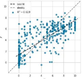
Figure 4: Prediction error of our regression model. On the x axis we show the actual values and on y axis we show the predicted values for each student on the testing set.
In this sense, in Figure 4, we plot the actual grade (y) of each student on the x axis, whilst on y axis we plot the grades predicted (𝑦𝑦�) by our model. Moreover, we show a dashed 45-degree line (identity) to compare with our model’s best fit prediction (best fit). Using this we can inspect the amount of variance in our regression model, i.e., where the model makes bigger mistakes and where the model hits. To illustrate, there are many points close to the identity, which means that the residual of the prediction is close to zero. However, we can observe a few outliers along a range of the target domain, which might explain the high value of our MAE. To illustrate, notice the density of errors on the point zero of the x axis forming a kind of a ‘vertical line’, which means that the model predicted higher grades for some students who achieved an actual grade close to zero. A possible explanation for that is that we are using data from the very beginning of the course (first two weeks) and, hence, some students might begin the course with effective behaviours that probably would lead to success. However, during the course they might give up because of personal reasons or even become less engaged and dropout. As instructors, we know empirically that students can change their posture in terms of engagement during the course, i.e., they can begin well but end up failing. We can also observe in this figure a few cases of the opposite phenomenon, i.e., students who achieved higher grades but the model predict low grades to them, which likely means that these students begin with bad habits but end up passing with higher grades because of possible changes on habits. As such, for regression, we believe that our model predictions are not highly accurate for extreme values (0's and 10's) because of those uncontrollable and unknown factors influencing the students’ grades, typical in human sciences. However, we believe that when using our regression model combined with teachers, these estimator errors for extreme values (0’s and 10’s) will be detected by the teachers ’intuition and experience with students, thus lessening the limitations of our regression model.
In Figure 5 we can see the residuals are proportionally distributed along the zero axis, which indicates there is no heteroskedasticity. To confirm that, we applied Goldfeld-Quandt test, and we did find homoscedasticity (p-value = 0.3471). Besides that, Figure 6 shows the residuals of our model on y axis and the actual students’ grades on the x axis. With this in hand, we can
739
perform a visual inspection of the regions within more or less errors regarding to the students’ grades prediction, confirming what we explained previously about our prediction on extreme grades (0’s and 10’s). Nonetheless, we can see that in overall the points are close to the horizontal black line (point zero on y axis), which means lower errors. Moreover, we claim that the regularization was done properly as the predictions on the training and testing set have almost the same spectrum and residual distribution (see the histogram), demonstrating that our model generalises well. Still, the histogram of the residuals shows a distribution centred on zero and with a bell shape, which suggests a linear underlying nature of the data.
Figure 5: Residuals of our regression model.
Figure 6: Prediction error of our regression model. 4.3 Analysis of Feature Effects on the Regression Outcomes
In this subsection, we answer our third research question (RQ3): ‘How we can interpret the results
740
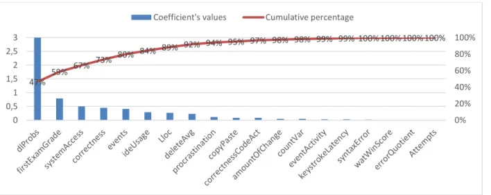
Figure 7: Pareto plot of the feature’s relevance based on their coefficients.
A better understanding of what students programming behaviours might be positive or negative and what goes behind the students’ grades could lead to a better analysis of which strategies we might use to teach and how our students would like to learn. As such, in this subsection, we go beyond prediction and move towards analysing the effects of features in our regression model outcome with the aim at understanding the major factors that can lead to success and failure in our cohort. To do so, we will analyse the coefficients of our regression model. Figure 7 shows a Pareto plot with the cumulative relevance of each feature, measured by the absolute value of each coefficient. We can see that the dlProbs (predicted probability from the DL model), is the most influential factor, being responsible for 47% of the prediction’s weight, which shows the technique of stacking works as we expected. In addition, the features dlProbs,
firstExamGrade, systemAccess, correcteness and events accomplish for 80% of the predictive
power of the model, which follows the Pareto’s Principal, or the 80/20 Pareto’s rule, which states that, in general, 80% of the effects come from 20% of the causes (Newman, 2005), in our case 20% of the features.
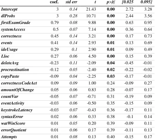
Moreover, in Table 7, we show the coefficients values, their confidence interval, statistics, and their statistical significance. A simple way to interpret these coefficients is the higher the absolute value the higher effect on the model outcome. To illustrate, for every additional degree (increase by one std as we used z-score standardisation) of ideUsage, the expected increase on final grade is something between [0.09-0.49] (95% C.L.), or 0.29 on average, keeping all other variables constant. With this in mind, the top features with higher impact are, respectively,
dlProbs (predicted probability from the DL model), firstExamGrade, systemAccess, correctness, events, ideUsage, and lloc. First, dlProbs is the most influential factor which shows the technique
of stacking works as we expected. Following, all the other top features have a positive magnitude which means that the greater the value the higher the positive effect regarding to the final grade of students. About firstExamGrade and correctness appearing the top features was only a confirmation, as we expected the students who do well on the first exam and assignment tend to perform better. However, as a more hidden pattern found, we can see that coding activity also plays an important role (systemAccess, events, ideUsage, and lloc) for student success. In other words, it suggests that it is important for learners to access (systemAccess) regularly the online judge actively (high events, ideUsage, and lloc), that is, solving the problems from the assignments with a reasonable number of logical lines of code (lloc), and spending time on the IDE with a considerable number of events generated (events), which means that the student is typing something on the IDE while he/she is accessing the online judge.
47% 59% 67% 73% 80% 84% 89% 92% 94% 95% 97% 98% 98% 99% 99% 100%100%100%100% 0% 20% 40% 60% 80% 100% 0 0,5 1 1,5 2 2,5 3
741
Table 7: Coefficients of our regression model. Statitiscally significan coefficients bolded (p-value<0.05).
coef. std err t p>|t| [0.025 0.095] Intercept 3 0.14 21.43 0.00 2.72 3.28 dlProbs 3 0.28 10.71 0.00 2.44 3.56 firstExamGrade 0.79 0.08 9.88 0.00 0.63 0.95 systemAccess 0.5 0.07 7.14 0.00 0.36 0.64 correctness 0.45 0.14 3.21 0.00 0.17 0.73 events 0.41 0.14 2.93 0.01 0.13 0.69 ideUsage 0.29 0.1 2.90 0.01 0.09 0.49 Lloc 0.27 0.06 4.50 0.00 0.15 0.39 deleteAvg -0.23 0.11 -2.09 0.04 -0.45 -0.01 procrastination -0.12 0.05 -2.40 0.02 -0.22 -0.02 copyPaste -0.09 0.04 -2.25 0.03 -0.17 -0.01 correctnessCodeAct 0.09 0.09 1.00 0.24 -0.09 0.27 amountOfChange 0.05 0.06 0.83 0.28 -0.07 0.17 countVar -0.05 0.07 -0.71 0.31 -0.19 0.09 eventActivity -0.03 0.06 -0.50 0.35 -0.15 0.09 keystrokeLatency -0.03 0.07 -0.43 0.36 -0.17 0.11 syntaxError 0.02 0.06 0.33 0.38 -0.1 0.14 watWinScore 0.01 0.05 0.20 0.39 -0.09 0.11 errorQuotient 0.01 0.06 0.17 0.39 -0.11 0.13 Attempts 0.01 0.08 0.13 0.40 -0.15 0.17
The other features that follow are, respectively, deleteAvg, procrastination and copyPaste. These three features have a negative coefficient, which means that lower values are better. As such, these coefficients might suggest that procrastination and a higher number of copyPaste on the first code solutions of an introductory programming course are not desirable programming behaviours. Furthermore, a high value of deleteAvg might indicate that students are struggling, by deleting the code and redoing it repeatedly.
Finally, features with less impact (no statistical significance, p-value >> 0.05) on the model outcome are: correctnessCodeAct, amountOfChange countVar, keystrokeLatency,
eventActivity, syntaxError, watWinScore, attempts, and errorQuotient. This is interesting, since
the literature (Jadud, 2006; Edwards et al., 2009; Watson et al. 2013; Leinonen et al., 2016; Carter et al., 2019; Pereira, 2019b) report that these features are generally useful to predict student’s performance. However, for this cohort and for our regression problem, this is not the case. A possible reason is that, again, we are dealing with data from the first two weeks of the course and, hence, some patterns are still not evident yet. For example, repeating the same errors (errorQuotient, SyntaxErrors, watWinScore) could not be a common behaviour in the beginning of the course because the problems are very easy. However, when the problems become more challenging, these students would need to use debugging tools, otherwise they might be stuck with the same errors increasing the value of metrics that compute errors.
With this understanding of negative and positive programming behaviours in hand, early interventions can be performed. To illustrate, learning analytics tools can be applied to monitor the students’ performance in relation to procrastination, copyPaste, etc. giving them a personalised feedback when they are in a situation of high risk of failing in the course. On the other hand, positive behaviour such solving many (higher correctness) problems soon (lower procrastination) can be encouraged in order to increase students’ motivation and self-regulation.
In closing, these features may not have a high relevance in isolation; however, together they have a reasonable predictive power for classification and regression. We believe that these
742
top features might be generalised for other contexts, as they don’t depend on nuances of a given compilation message or a specific programming language or web-based system. Moreover, two of our extended features (amountOfChange and eventActivity) were not statistically significant for our regression model, which indicates there is no linear relationship with the students’ final grades and these two features. However, the classification results, which were achieved using non-linear algorithms, improved using our extended features, which may suggest a non-linear relationship.
4.4 Pedagogical Implication of Early Prediction
Robins (2019) and Freitas & Pereira (2019) advocate about the importance of students solving many problems to improve their programming skills. However, this leads to a significant increase on the workload of instructors, as they need to evaluate many codes from many students. In this sense, the use of online judges in CS1 courses are gaining momentum (Ihantola et al., 2015; Galvão et al., 2016; Junior & Pereira, 2019), since they bring benefits in decreasing instructors/monitors workload and enable a data-driven analysis of CS1 students’ behaviours. Blikstein et al. (2014) and Carter et al. (2019) explain that such analysis allows a formative assessment, as not only the code submitted by the learners can be evaluated, but also the process behind it, when students are building their code.
Moreover, in programming classes, we teach our students to be excellent problem solvers. According to the SOLO taxonomy, this represents the highest level of abstraction. SOLO (Biggs & Collis, 1982), which stands for Structure of the Observed Learning Outcome, is a general education framework that describes levels of increasing complexity in a learner’s understanding of a subject. It ranges from pre-structural (no understanding), to unistructural, multistructural, relational, and extended abstract (understanding at a high level that enables generalisation to a new topic or area). Although instructors of CS1 classes aim to bring all students to the extended abstract level, many students will probably remain at the lower levels.
In our work, we aim at high SOLO levels by using a methodology based on practice and formative assessment. As explained by Robins (2019), hands-on experience is the most effective form of learning for students. Thus, in the 7 sessions of the CS1 program, we propose many assignments and exams, always with a close tutoring, allowing a formative, beside the summative assessment. In other words, the fine-grained data collect from our online judge allows for a formative assessment, as not only the code submitted by the students can be evaluated, but also the process behind it. This kind of assessment provides a comprehensive view upon the student’s learning and can guide the teacher towards truly effective interventions.
Additionally, with early prediction, in a standard course, teachers could provide extra assignments for the high-achieving group and personalised support to those who are struggling. If the strategies of effective novices can be identified, it may be possible to promote effective strategies to all groups. Such early prediction allows personalised feedback, but this is not scalable to large classes without proper technological support. With an approach such as ours, effective and ineffective behaviours can be automatically identified early on, and encouraged or discouraged, respectively. Such process of early intervention can be performed using dashboards, e-mails, etc. In other words, as ‘prevention is better than a cure’, likewise, it is better to prevent students from failure as soon as possible, instead of finding out students are struggling when their poor marks come in.
Moreover, this approach prevents fragile learning (Robins, 2019). This occurs when students pass by learning in a short period something that they should have learn over the entire course (by ‘cramming’ at the end). As such, it is crucial to decrease the time lag between detecting at-risk students and acting to provide early help to the learner.
Importantly, according to Ihantola et al. (2015), this kind of approach presents essential benefits for the educational context: