www.hydrol-earth-syst-sci.net/16/3011/2012/ doi:10.5194/hess-16-3011-2012
© Author(s) 2012. CC Attribution 3.0 License.
Earth System
Sciences
Are drought occurrence and severity aggravating? A study on SPI
drought class transitions using log-linear models and ANOVA-like
inference
E. E. Moreira1, J. T. Mexia1, and L. S. Pereira2
1CMA – Center of Mathematics and Applications, Faculty of Sciences and Technology, Nova University of Lisbon, 2829-516 Caparica, Portugal
2CEER – Biosystems Engineering, Institute of Agronomy, Technical University of Lisbon, Tapada da Ajuda, 1349-017 Lisboa, Portugal
Correspondence to: E. E. Moreira ([email protected])
Received: 30 November 2011 – Published in Hydrol. Earth Syst. Sci. Discuss.: 19 December 2011 Revised: 5 July 2012 – Accepted: 25 July 2012 – Published: 28 August 2012
Abstract. Long time series (95 to 135 yr) of the 12-month
time scale Standardized Precipitation Index (SPI) relative to 10 locations across Portugal were studied with the aim of investigating if drought frequency and severity are chang-ing through time. Considerchang-ing four drought severity classes, time series of drought class transitions were computed and later divided into several sub-periods according to the length of SPI time series. Drought class transitions were calcu-lated to form a 2-dimensional contingency table for each sub-period, which refer to the number of transitions among drought severity classes. Two-dimensional log-linear models were fitted to these contingency tables and an ANOVA-like inference was then performed in order to investigate differ-ences relative to drought class transitions among those sub-periods, which were considered as treatments of only one factor. The application of ANOVA-like inference to these data allowed to compare the sub-periods in terms of prob-abilities of transition between drought classes, which were used to detect a possible trend in droughts frequency and severity. Results for a number of locations show some simi-larity between alternate sub-periods and differences between consecutive ones regarding the persistency of severe/extreme and sometimes moderate droughts. In global terms, results do not support the assumption of a trend for progressive ag-gravation of drought occurrence during the last century, but rather suggest the existence of long duration cycles.
1 Introduction
Drought is a normal recurrent feature of climate, which oc-curs in all climatic zones, though with varied characteristics. There are many definitions of drought, often related with the sector perceiving or being impacted by it, thus leading to de-fine meteorological, agricultural, hydrological and socioeco-nomic droughts (Dracup et al., 1980; Tate and Gustard, 2000; Mishra and Singh, 2010). In this study, the definition pro-posed by Pereira et al. (2009) is assumed: drought is a nat-ural but temporary imbalance of water availability, consist-ing of a persistent lower-than-average precipitation, of un-certain frequency, duration and severity, of unpredictable or difficult to predict occurrence, resulting in diminished wa-ter resources availability and reduced carrying capacity of the ecosystems, thus affecting socioeconomic activities and the society. Short dry periods or dry spells, often also called droughts, are therefore not considered in our analysis. As-sessing changes in drought frequency and severity, possibly aggravating with time, is important to develop related risk management issues.
There are various drought indices for assessing drought severity (Heim, 2002; Keyantash and Dracup, 2002; Mishra and Singh, 2010). Drought indices are numerical indica-tors incorporating or derived from hydro-meteorological in-dicators. Meteorological drought indices respond to weather conditions that have been abnormally dry or abnormally wet. Precipitation based drought indices are the first indi-cators of droughts, since hydrological droughts may emerge
considerable time after a meteorological drought has been established (Wilhite and Buchanan-Smith, 2005). Conse-quently, precipitation-based drought indicators are the basic tools for a drought early warning system. Examples are the Standardized Precipitation Index, SPI (McKee et al., 1993, 1995), the Palmer Drought Severity Index, PDSI (Palmer, 1965) or a modified version of this index for Mediterranean conditions, MedPDSI (Pereira et al., 2007; Martins et al., 2012).
The SPI is often used for the identification of drought events and to evaluate their severity through well defined drought classes (McKee et al., 1993, 1995). The SPI is widely used because it allows a reliable and relatively easy comparison between different locations and climates (Bordi et al., 2009). It has the advantage of statistical consistency and the ability to reflect both short-term and long-term drought impacts (Steinemann et al., 2005) since it may be computed on shorter or longer time scales, which reflect dif-ferent lags in the response of the water cycle to precipitation anomalies. Another advantage of SPI is that, due to its stan-dardization, its range of variation is independent of the ag-gregation time scale of reference, as well as on the particular location and climate. Therefore, SPI values are suited to be used as drought triggers, i.e. thresholds that determine when drought management actions should begin and end (Steine-mann et al., 2005). The stochastic properties of the SPI time series can be used for predicting short term drought class transitions, thus assisting in drought management (Moreira et al., 2008a; Paulo and Pereira, 2008). The 12-month time scale, as well as larger time scales, identifies anomalous dry periods of long duration and relates well to the conditions assumed in the adopted definition, i.e. with the impact of drought on hydrologic regimes and water resources of a re-gion, as pointed out by Vicente-Serrano (2006), or to the ef-fects of fluctuation in rainfall over short intervals (Mishra et al., 2009). Shorter time scales of 3 to 6 months are more use-ful to detect agricultural droughts and longer ones may be useful to consider impacts on groundwater resources. For the Portuguese conditions, where a dry period of near 6 months occurs, droughts impacting the hydrologic regime are bet-ter assessed when using the 12-month time scale (Paulo and Pereira, 2006). Hence, former studies on drought variability or on prediction of drought class transitions were performed with the SPI 12-month (Moreira et al., 2006, 2008a; Paulo and Pereira, 2008).
It is generally accepted that there is an intensification of the global water cycle due to climate change, particularly as-sociated with global warming, which can cause an increase in droughts occurrence and severity, though highly variable among regions (Huntington, 2006). This perception is com-mon to various studies forecasting droughts and dry weather conditions as influenced by climate change, e.g. Burke et al. (2006), Lehner et al. (2006), Beniston et al. (2007) and Heinrich and Gobiet (2011). However, there is not a common view on the drought concepts used by the various researchers,
and often dry spells are considered to support a foreseen in-crease in dryness for Europe (Heinrich and Gobiet, 2011). An increase in awareness on water problems and of press information about droughts also lead to an increased public perception that droughts may be aggravating (Ruiz Sinoga and Gross, 2012).
Results of various studies at global, European, Iberian or Portuguese levels do not confirm the hypothesis of drought aggravation but often lead to contradictory conclu-sions since a strong spatial variability is generally encoun-tered. The world scale drought studies by Dai et al. (2004) and Dai (2011) using the PDSI identified spatial variabil-ity and show trends for dryness in various regions includ-ing the Mediterranean region and trends for wetness in other regions such as in northern Eurasia. Relative to Europe and the 20th century, Lloyd-Hughes and Saunders (2002) found a greater frequency of extreme droughts in eastern Europe and, conversely, less frequent droughts in northwest Euro-pean seaboard, the Mediterranean seaboard and the Alps. They also found that results of SPI-12 were nearly identi-cal to those obtained from the PDSI. Bordi et al. (2009), us-ing the SPI and a non-linear trend analysis, found that over-all trends for dryness in Europe were inverted in the last decade, i.e. time variability of trends is added to the spatial variability. It is interesting to note a recent interpretation of the spatial variability of droughts at a large scale as resulting from the combination of multiple small area events (Lloyd-Hughes, 2012).
Various studies refer to the Mediterranean region and show that time variability and trends are associated with spa-tial variability (Vicente-Serrano, 2006; Vicente-Serrano and Cuadrat-Prats, 2007). These results agree with the referred interpretation by Lloyd-Hughes (2012). Sousa et al. (2011) used the self-calibrated PDSI for the period 1901–2000 and found a clear trend towards drier conditions in most of the western and central Mediterranean, excepting the north-western Iberian Peninsula. They found that the North At-lantic Oscillation (NAO) correlates negatively with the PDSI, while the Scandinavian pattern is positively correlated. Var-ious other studies identify dryness relationships with NAO (e.g. Rodrigo et al., 2000; Nicault et al., 2008; Santos et al., 2010). Large time scale analysis shows that a large pe-riod fluctuation of dryness and wetness has occurred in the Mediterranean area. Nicault et al. (2008) refer that the ampli-tude and variation of the PDSI during the 20th century were similar to those of the 16th and 17th centuries; however, a trend for PDSI decrease was observed in the last decades, particularly in the western Mediterranean region. Relative to central Mediterranean, in agreement with the results by Sousa et al. (2011), negative trends were identified in south-ern Italy (Bonaccorso et al., 2003; Piccarreta et al., 2004; Bordi et al., 2007).
Droughts in the the Iberian Peninsula were studied by Vicente-Serrano et al. (2011), who adopted SPI and SPEI, an index derived from SPI by considering evapotranspiration.
They found that droughts did not increase in northwestern Iberian Peninsula during 1930–2006 contrarily to the trends observed in other Iberian regions, such as the Ebro basin and the Tagus basin. However, Rodrigo et al. (2000) per-formed an analysis of rainfall variability in southern Spain on decadal and centennial scales and found an alternation of wet and dry periods, with various decades of duration. They also found that rainfall anomalies in the 20th century show a behaviour similar to other periods in the past. Rela-tive to southern Portugal, Alcoforado et al. (2000) also found that rainfall variability in the past (late Maunder Minimum) was similar to the present, with alternation of dry and wet periods. Santos et al. (2011) applied Principal Components Analysis (PCA) to a good number of rainfall stations in Por-tugal and found no significant trends for increased severity of droughts identified with the SPI computed with various time scales and using the Mann-Kendall (MK) trend test. Mar-tins et al. (2012) also applied PCA and analysed the linear trends to the first and second PC scores of SPI-12, PDSI and MedPDSI indices applied to Portugal and found no signifi-cant increases in droughts. Paulo et al. (2012) used the MK trend test to the Portuguese weather stations and found sig-nificant trends for temperature increases in the majority of lo-cations but contradictory results for the precipitation trends. They also applied the MK trend test to SPEI and MedPDSI and found only a few cases with trends indicating significant drought severity aggravation. However, these results were obtained with shorter time series than those considered in the current study. Results of former studies with log-linear mod-els led to conclude that droughts are not more frequent or have an increased severity (Moreira et al., 2006); however, the need for considering longer time series was then iden-tified. A possible occurrence of cycles in precipitation has been detected (Moreira et al., 2008b), which could be inter-preted as leading to a cyclic aggravation and attenuation of drought severity. More recent studies agree with that hypoth-esis (Santos et al., 2010). Therefore, considering that results are contradictory in terms of trends for droughts aggravation or attenuation, that droughts show a very strong spatial vari-ability that influences a temporal analysis, and that the time variability of droughts is possibly associated with cycles of dryness and wetness, the need for an innovative and accurate analysis for detection of trends using long time series of SPI was identified.
The most common methods used in hydrology and clima-tology to assess trends in time series are the tests for trend significance like Mann-Kendall (Helsel and Hirsch, 1992). These non-parametric tests are based on the calculation of Kendall’s tau measure of association between two samples and they have been applied to drought indices trend detec-tion (Piccarreta et al., 2004; Sousa et al., 2011; Paulo et al., 2012). The fitting of linear and non-linear regression models to time series is also usually used for the posterior identifi-cation of the model tendency (Mazvimavi, 2010; Reiser and Kutiel, 2005; Shao et al., 2011). Several authors have used
PCA, a multivariate statistical technique, to observe the spa-tial and temporal variability of drought and then draw tem-poral patterns from the data (Bordi et al., 2004, 2006; Ra-ziei et al., 2009; Santos et al., 2010; Martins et al., 2012). In atmospheric and climate sciences, the PCA’s are com-monly called empirical orthogonal functions (EOF), and are often used with the principal objective of extracting com-mon space-time features from within the data (Burke et al., 2006; Dai et al., 2004; Lloyd-Hughes, 2012; Vicente-Serrano and Cuadrat-Prats, 2007). However, the choice of the tech-nique to assess space-time relationships is limited and they have some difficulties regarding the interpretation of the re-sultant patterns. So, Lloyd-Hughes (2012) proposed a sim-ple agglomerative technique to identify large-scale coherent space-time drought events. Once a set of coherent space-time events has been identified it is possible to test for similarities in their structure using measures of similarity.
With the aim of extracting temporal patterns, the Fourier decomposition of time series used in spectral analysis can be applied to assess cycles of extreme events and recognize their return periods (Moreira et al., 2008b). The statistics of extremes has been widely used to study hydrologic extremes (Katz et al., 2002; Shang et al., 2011). Using extreme value theory, Bordi et al. (2007) studied the extremes of the SPI and mapped the return periods of extreme wet and dry events. A probabilistic approach using an alternative renewable process and run theory was used by Mishra et al. (2009) to investigate the mean drought interarrival time and the SPI transitions probabilities of drought events.
The analysis of variance, which includes F tests, is not commonly used for detection of trends in hydrology and cli-matology. However, some applications can be found. Ro-drigo et al. (2000) used t-tests and F tests to compare the rainfall means and standard deviations of the alternate dry and wet phases detected in a 500-yr reconstructed rainfall period for southern Spain. Suhailaa et al. (2011) used func-tional data analysis and one way funcfunc-tional analysis of vari-ance to compare rainfall patterns between regions and could find significant differences between regions.
The general purpose of the current study is to analyse the historical frequency and duration of meteorological drought in Portugal. In particular, the objective is to detect the pos-sible occurrence of large cycles originated by a natural vari-ability or, instead, a trend in time evolution of drought fre-quency and severity through the analysis of drought class transitions and to test a new methodology. The analysis is based on the SPI, due to its above mentioned advantages, and in log-linear modelling, which has shown to be an ade-quate tool for drought class transitions analysis and for short-term forecast of SPI class transition probabilities (Moreira et al., 2006, 2008a). The log-linear modelling, applied on the contingency tables for SPI drought class transitions, was used to obtain probability ratios, named odds, and their con-fidence intervals, that allowed the comparison of different sub-periods of the same time series (Moreira et al., 2006).
However, the odds confidence intervals sometimes were too large, therefore not reliable enough. Adopting a more robust statistical analysis when comparing sub-periods was consid-ered appropriate. Since log-linear models proved well for analyzing and predicting transitions between successive SPI drought classes (Moreira et al., 2006, 2008a), the adjusted models were used as a base for the current ANOVA-like in-ference approach. In particular, the ANOVA was used to test whether the persistence or transitions in drought classes are significantly different between sub-periods over the last cen-tury, in order to assess the presence of trends or cyclic be-haviour in droughts occurrences. The combined use of log-linear modelling and ANOVA-like inference allows to cap-ture an accurate portrait of the past frequencies of drought class transitions and, then, use this portrait in the ANOVA algorithms in order to obtain reliable results about the vari-ability of drought class transitions. Hence, this study intends to detect possible trends in drought aggravation decompos-ing long SPI time series into sub-periods that could relate to a cyclic alternation of dryness and wetness. The study ap-plies log-linear modelling to characterize transitions within each sub-period and ANOVA-like inference to recognize the significant differences among such sub-periods.
2 Data, SPI time series and division in sub-periods
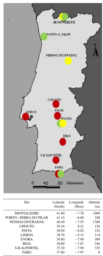
The data used in this study are constituted by long time series of monthly Standardized Precipitation Index in a 12-month time scale (SPI-12) for 10 meteorological stations located in Portugal (Fig. 1).
The time series duration varies between 95 and 135 yr. The identification and time series duration for each station are presented in Table 1. The 12-month time scale was se-lected considering the fact that this time scale corresponds to a drought duration that may impact the hydrological cycle and balance as well as the results previously obtained with the SPI-12 as discussed in the previous section.
The methods used to assess the quality of precipitation data series and to compute the SPI at the 12-month time scale are described in Paulo et al. (2003, 2005). The annual pre-cipitation data sets used in SPI computation were obtained from monthly data and were investigated for randomness and homogeneity using the autocorrelation test (Kendall τ ) and the homogeneity tests of Mann-Whitney for the mean and the variance (Helsel and Hirsch, 1992). The test results have shown that all data sets have good quality and therefore none of the time series was rejected. The appropriateness for using the gamma distribution to compute the 12-month time scale (SPI-12) was verified using non-parametric tests, namely the Chi-square test. SPI computation is described in former stud-ies (Paulo et al., 2003, 2005). In this study, the reference period for standardization and computation of the SPI was the whole observation period. Considering that the time se-ries have different lengths, this fact did not have influence on
Site Latitude Longitude Altitude
(North) (West) (m) MONTALEGRE 41.80 −7.78 1069 PORTO−SERRA DO PILAR 41.10 −8.60 100 PENHAS DOURADAS 40.40 −7.55 1388 CHOUTO 39.16 8.21 126 PAVIA 38.90 −8.02 192 LISBOA 38.70 −9.15 114 EVORA 38.60 −7.90 309 BEJA 38.00 −7.87 246 S.B.ALPORTEL 37.20 −7.90 325 FARO 37.00 −7.97 8
Fig. 1. Portugal (location of the stations). The colors refer to the type of behaviour shown by drought dynamics in each location as described in Fig. 4 and analysed for each location in Figs. 5 and 6. Red circles refer to a cycles behaviour, yellow to a trend for aggra-vation, blue for a decreasing trend and green for no trend nor cyclic behaviour; mixed colors indicate that no clear typical behaviour was detected.
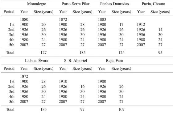
Table 1. Division into 4 or 5 sub-periods according to each time series total duration.
Montalegre Porto-Serra Pilar Penhas Douradas Pavia, Chouto Period Year Size (years) Year Size (years) Year Size (years) Year Size (years)
1880 1872 1883 1st 1900 20 1900 28 1900 17 1912 2nd 1926 26 1926 26 1926 26 1926 14 3rd 1956 30 1956 30 1956 30 1956 30 4th 1980 24 1980 24 1980 24 1980 24 5th 2007 27 2007 27 2007 27 2007 27 Total 127 135 124 95
Lisboa, ´Evora S. B. Alportel Beja, Faro Period Year Size (years) Year Size (years) Year Size (years)
1872 1st 1900 28 1910 1900 2nd 1926 26 1926 16 1926 26 3rd 1956 30 1956 30 1956 30 4th 1980 24 1980 24 1980 24 5th 2007 27 2007 27 2007 27 Total 135 97 107
Table 2. Drought classification of SPI (modified from Mckee et al., 1993).
Code Drought classes SPI values
1 Non-drought SPI ≥ 0
2 Near normal −1 < SPI < 0 3 Moderate −1.5 < SPI ≤ −1
4 Severe/Extreme SPI ≤ −1.5
results because the SPI time series and the respective tran-sitions were not compared among locations, but among the sub-periods within each time series. Nevertheless, no esti-mation bias are expected in computation of SPI due to differ-ent lengths of time series, or they are very small, because all time series are quite long and therefore the fitting parameters of the probability distribution functions change very little.
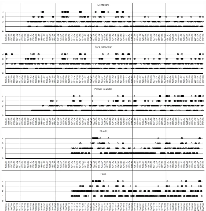
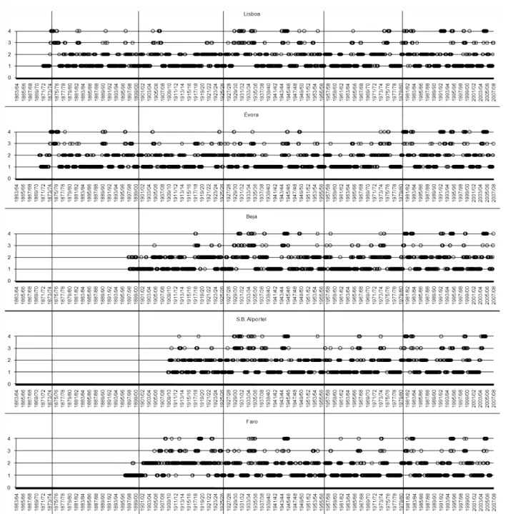
The SPI time series were converted into drought classes (Figs. 2 and 3). The severity of drought classes adopted are defined in Table 2; they were modified from those proposed by McKee et al. (1993, 1995) by grouping the severe and ex-tremely severe drought classes. This modification was done for modelling purposes since transitions referring to the ex-tremely severe drought classes are much less frequent than for other classes; thus, a possible bias is avoided since too many zeros in the contingency tables may cause problems in the fitting.
In order to perceive if there is a trend for drought ag-gravation, a statistical comparison was made between sub-periods of each time series, which are taken as treatments
for the ANOVA application. The large duration time series (from 1872 to 2007) were divided into 5 sub-periods and the shorter time series of near 100 yr duration were divided into 4 sub-periods. The time series division into 5 or 4 dif-ferent sub-periods is presented in Table 1. Within each time series, the sub-periods have different sizes, but the beginning and ending year of each sub-period is the same in all loca-tions with exception of the first sub-period that depends on the first year of each series (Table 1). The sizes of the sub-periods range from 24 to 30 yr. However, the first sub-period of each time series is sometimes smaller than 24 because of the different lengths of the time series. The choice of those sub-periods were based upon the results obtained in a former study (Moreira et al., 2006), where a possible existence of a cycle was uncovered. In that study, which used shorter time series, these were divided into 3 sub-periods of similar du-ration (22/23 yr) because 3 was the minimal number when trying to find either a cycle or a trend. However, if there is a cycle, it is not expectable that periods of drought recurrence should have exactly the same duration in every location but it is more likely that they refer to a larger range (Moreira et al., 2008b). The results obtained from the spectral analysis of the time series of annual precipitation regarding the 22 stud-ied sites in southern Portugal show that the return period of severe/extreme droughts tend to range from 10 to 15 yr (Mor-eira et al., 2008b). Periodicities of the same magnitude were observed by other authors (Bonaccorso et al., 2003; Bordi et al., 2007; Santos et al., 2010). Therefore, sub-periods were selected from the observation of the time series of drought classes (Figs. 2 and 3) with the duration of sub-periods in
Fig. 2. Drought classes (Table 2) through time by location (sub-periods are indicated with vertical lines).
a range double of that identified by spectral analysis and in agreement with those used in the log-linear study by Moreira et al. (2006).
If some sites show a significant trend for progressive in-creasing or dein-creasing in droughts occurrence and severity, the successive sub-periods should present significant differ-ences between them. Contrarily, if a significant trend does not exist, then those differences between successive sub-periods should not be significant. Except for the sites in northern Portugal, it can be observed that there are sub-periods with fewer events of moderate and severe/extreme
droughts than those observed in previous and subsequent sub-periods (Figs. 2 and 3).
When using analysis of variance, it is usual to formu-late the hypothesis to be verified according to our expec-tations. In the present case, based upon former studies, the hypothesis to be tested is that of existing trends or rather cycles of occurrence of severe/extreme droughts. Therefore, the sub-periods were considered as treatments for a one-way ANOVA, which uses the F tests and the methods of mul-tiple comparison (Scheff´e, 1959). In order to test the ex-istence of significant differences between sub-periods, the
Fig. 3. Drought classes (Table 2) through time by location (cont.) (sub-periods are indicated with vertical lines).
null hypothesis is formulated to reflect the absence of sig-nificant differences against the alternatives of the existence of a trend for drought aggravation/attenuation or a cycle of severe droughts. The differentiation between a trend or a cy-cle can only be done through the use of the Scheff´e multiple comparison method as analysed in Sect. 3.2.
3 Modelling and methods of analysis
After dividing the time series, the number of one step tran-sitions between any drought class was counted for each sub-period in order to form a 2-dimensional 4 × 4 contingency table with N = 16 cells. An example of these contingency tables is presented in Table 3, where 5 contingency tables result from dividing the Porto time series into 5 sub-periods. The observed frequencies, denoted by nh,j, h, j = 1, ..., 4
on the contingency tables, are the number of times that the drought class h occurs in a given month followed by the
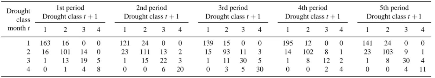
Table 3. Contingency tables resulting from the division of the Porto time series into 5 sub-periods.
Drought 1st period 2nd period 3rd period 4th period 5th period class Drought class t + 1 Drought class t + 1 Drought class t + 1 Drought class t + 1 Drought class t + 1 month t 1 2 3 4 1 2 3 4 1 2 3 4 1 2 3 4 1 2 3 4
1 163 16 0 0 121 24 0 0 139 15 0 0 195 12 0 0 141 24 0 0 2 16 101 14 0 23 111 13 2 15 93 11 3 14 102 8 1 23 103 9 1 3 1 13 19 5 1 15 22 3 1 11 30 5 1 8 12 2 1 8 30 4 4 0 1 4 8 0 0 6 20 0 3 5 30 0 0 2 4 0 0 4 11
drought class j in the next month (number of transitions be-tween drought classes in successive months). In each pair of consecutive months, the first one is the entry month, while the other is the exit month.
Since the sub-periods have different sizes, the observed frequencies were weighted in order to make it possible for the comparison between the 5 (or 4) sub-periods in terms of the number of drought class transitions.
The log-linear modelling used next allowed the applica-tion of an ANOVA-like inference to compare the expected frequencies among the sub-periods. This modelling approach was required because, unlike the observed frequencies, the modelled expected frequencies meet the assumptions of nor-mality and independence of the observations required to apply the analysis of variance.
3.1 Log-linear modelling
Log-linear models were fitted to contingency tables relative to all weather stations. The adjusted models were used to carry out an ANOVA-like inference to compare the 4 or 5 sub-periods of each data series. These sub-periods corre-spond to the treatments of a one-way ANOVA.
Previous studies (Moreira et al., 2006, 2008a) led to ad-just to similar two-dimension contingency tables the quasi-association (QA) log-linear models (Agresti, 1990). Denot-ing by mh,j the mean value E(nh,j) of nh,j with h, j =
1, ..., 4, which is also called expected frequency, the QA log-linear models for two-dimension contingency tables have the following formulation
wh,j=log mh,j=λ + λrh+λ c
j+β × h × j + δhI (h = j ) (1)
where λ is the constant parameter also designated by the grand mean; λrh is the parameter representing the row ef-fect, i.e. the effect of drought class h of the entry month,
h =1, ..., 4; λcj is the parameter representing the column ef-fect, i.e. the effect of drought class j of the exit month,
j =1, ..., 4; β is the linear association parameter between rows and columns; δh is a parameter related to the h-th
di-agonal element of the contingency table, h = 1, ..., 4; and
I (h = j )is a function that takes the value 1 when the con-dition h = j holds and the value 0 otherwise. The expected frequencies mhj represent the expected number of
transi-tions between the drought classes h and j in two
consecu-tive months during each sub-period. The word “effect” refers to any deviation above the mean. The QA log-linear mod-els allow linear-by-linear association of the main diagonal of the contingency tables and are adequate to fit to squared ta-bles (when the number of columns and lines are equal) with ordered categories, resulting from a pairwise comparison of dependent samples, which is the case in this application.
When adjusting these models it is assumed that the nh,j,
h, j =1, ..., 4, are values taken by independent Poisson dis-tributed variables (Agresti, 1990). The assumption of in-dependency of the nh,j, h, j = 1, ..., 4 could be
consid-ered because transitions between drought classes in succes-sive months mainly depend on the amount of precipitation occurring in those months, not on transitions in previous months (Paulo and Pereira, 2007). Since the observed fre-quencies meet the assumptions of independent Poisson vari-ables, the maximum likelihood estimators (MLE) ˆλ, ˆλrh, ˆλcj,
ˆ
β, ˆδhand ˆmh,j, h, j = 1, ..., 4 of the model parameters could
be obtained.
In this modelling, the constraint
4 X h=1 λrh= 4 X j =1 λcj=0
is required in order to make the above parameters identifi-able (Agresti, 1990). As a consequence of that condition, the parameters λrh and λch with h = 1, ..., 4 are not linearly in-dependent among themselves; thus, to simplify the model it was taken λh1=λc1=0.
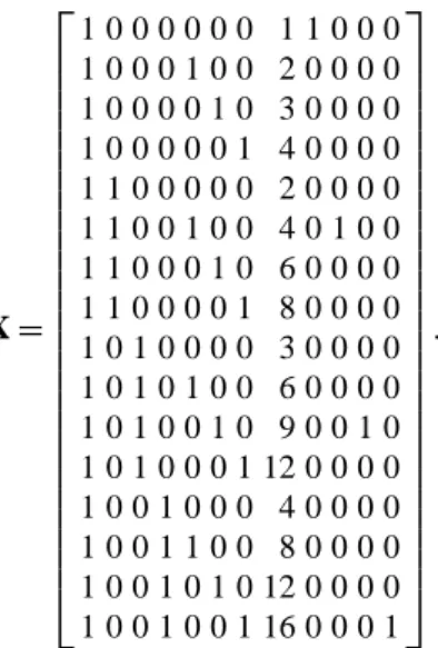
To ease the ANOVA computations and the presentation herein, a matrix notation was used. The linearly independent parameters in the model are 12 (λ, λr2, λr3, λr4, λc2, λc3, λc4,
β, δ1, δ2, δ3, δ4) and they constitute the parameter vector θ , whose components are θt, t = 1, ..., 12. The corresponding
maximum likelihood estimators of the parameters constitute the vector ˆθ . In order to rewrite the log-linear model in
ma-trix notation we define the vectors n, m and w as the vectors of observed frequencies, expected frequencies and of log-arithms of expected frequencies, respectively. The compo-nents of these vectors are now ordered according to the sole index l = 4h + j − 4. The model matrix, containing known
constants derived from Eq. (1), takes the form X = 1 0 0 0 0 0 0 1 1 0 0 0 1 0 0 0 1 0 0 2 0 0 0 0 1 0 0 0 0 1 0 3 0 0 0 0 1 0 0 0 0 0 1 4 0 0 0 0 1 1 0 0 0 0 0 2 0 0 0 0 1 1 0 0 1 0 0 4 0 1 0 0 1 1 0 0 0 1 0 6 0 0 0 0 1 1 0 0 0 0 1 8 0 0 0 0 1 0 1 0 0 0 0 3 0 0 0 0 1 0 1 0 1 0 0 6 0 0 0 0 1 0 1 0 0 1 0 9 0 0 1 0 1 0 1 0 0 0 1 12 0 0 0 0 1 0 0 1 0 0 0 4 0 0 0 0 1 0 0 1 1 0 0 8 0 0 0 0 1 0 0 1 0 1 0 12 0 0 0 0 1 0 0 1 0 0 1 16 0 0 0 1 .
Let’s designate the 12 components row vectors of X by xl
with l = 1, ..., 16. This matrix X is the same for all stations because it relates with the QA log-linear model and does not depend on the data set. The QA log-linear model in matrix notation is then
w = log m = Xθ .
Since a rather long time span is used, it may be assumed that: 1. the vector ˆθ of MLE estimates is asymptotically normal
with mean value θ and variance-covariance matrix
(XTD( ˆm)X)−1
where D( ˆm) is the diagonal matrix, whose principal
el-ements are the adjusted expected frequencies (Agresti, 1990);
2. the vector ˆθ is independent from the residual deviance
G2=2 16 X l=1 nllog(nl/ ˆml) =2 16 X l=1 nllog(nl) − 16 X l=1 nlwˆl !
obtained when adjusting a log-linear model to a con-tingency table and measures the goodness of fit. G2is asymptotically distributed as a central Chi-Square with 4 degrees of freedom since there are 16 cells in the con-tingency tables and 12 linearly independent parameters to be adjusted (Agresti, 1990; Nelder, 1974). Therefore, to validate the adjustment of the model, the Chi-Square test may be used with the statistic G2 (Agresti, 1990; Nelder, 1974). In the expression of G2the frequencies are also ordered according to index l.
Table A1 in the Appendix presents the adjusted parameters and the residual deviances for all stations and respective sub-periods.
Let’s designate by
ˆ
wl=xTl θ , l = 1, ..., 16ˆ
the components of vector ˆw of the logarithms of the expected
frequencies. These values are independent among themselves and since they are linear combinations of the model parame-ters they are also normal, with mean value wland variance
V ( ˆwl) =xTl (XTD( ˆm)X) −1x
l.
Thus, an ANOVA-like inference can be used to compare the expected frequencies between the sub-periods of the same time series since the normality and independence of the re-sponse variable (the logarithms of the expected frequencies) can be assumed.
3.2 One-way ANOVA-like inference and Scheff´e
multi-ple comparison method
The analysis of variance includes the F tests that have well known optimal properties (Lehmann, 1997; Ito, 1980), which extend to Scheff´e multiple comparison method (Scheff´e, 1959). Jointly, they are possibly the most powerful statisti-cal tool available for measuring differences between samples when comparing then.
In the current case study, ANOVA-like inference aims at finding significant differences between the sub-periods of each time series. The logarithms of the expected number of transitions between all drought classes were taken as obser-vations in an one-way ANOVA linear model with fixed ef-fects (Hocking, 2003). In order to perform the ANOVA to compare the logarithms of expected frequencies generated by the log-linear models fitted to the various sub-periods, some ANOVA algorithms had to be adapted.
Supposing a time series divided into 5 sub-periods, these were considered as treatments of one-way ANOVA (Mont-gomery, 1997). The expected frequencies generated by the log-linear model fitted to each sub-period can be considered independent from the expected frequencies generated by the log-linear model fitted to a different sub-period of the same time series, because, as said before, the transitions between drought classes in successive months do not depend on the amount of precipitation occurring on previous months but on that observed in the considered month. Thus, these values can be regarded as 5 independent samples for the purposes of ANOVA application.
Let the 5 sub-periods be indexed by i = 1, ..., 5, so the vec-tors ni, ˆmi and ˆwican be defined, as well as a matrix Y = [ ˆw1... ˆw5]T
with row vectors
yl= [ ˆwl,1... ˆwl,5] having mean vectors
with l = 1, ..., 16. If the 5 sub-periods are similar, the hypothesis
H0,l:wl,1=... = wl,5, l =1, ..., 16
will hold. This hypothesis may be rewritten as
H0,l:Aµl=0, l = 1, ..., 16
where the matrix A has, for instance, the following configuration A = 1 -1 0 0 0 1 0 -1 0 0 1 0 0 -1 0 1 0 0 0 -1
that serves to correctly formulate the hypothesis of equal-ity between the mean values wl,i with l = 1, ..., 16 and i =
1, ..., 5. The vectors ylare normal with mean vectors µl and
diagonal variance-covariance matrices, Dl, with principal
el-ements xTl (XTD( ˆm1)X)−1xl,..., xTl (XTD( ˆm5)X)−1xl, with l =1, ..., 16, independent from SG2= 5 X i=1 G2i
which is asymptotically distributed as a central chi-square with 20 degrees of freedom (Scheff´e, 1959). Thus, Ayl is
also normal with mean vector Aµl and variance-covariance
matrix ADlAT, l = 1, ..., 16. Therefore, when H0,t, with l = 1, ..., 16, holds, the statistics
Fl=
12 2
(Ayl)T(ADlAT)−1Ayl
SG2 , l =1, ..., 16
will have a central F of the Fisher-Snedecor distribution with 4 and 20 degrees of freedom (Scheff´e, 1959). The null hy-pothesis is rejected if the value of the Flstatistic exceeds the
5% quantil for the F distribution with 4 and 20 degrees of freedom (F0.05,4,20). In this way, an F test was obtained to test the null hypothesis of equality of expected frequencies between the sub-periods. When the hypothesis is rejected for a specific drought class transition, e.g. m3,4, it means that the sub-periods are not identical in terms of that ex-pected frequency. In these cases, the Scheff´e multiple com-parison method is used to find which differences between sub-periods are significant (Scheff´e, 1959).
When the time series were divided into 4 sub-periods, the vectors yland µlhave only with 4 components, a matrix
A = 1 -1 0 0 1 0 -1 0 1 0 0 -1
is used and the Fl statistic have a central F distribution with
3 an 16 degrees of freedom.
The Scheff´e multiple comparison method uses the inequality |dTyh|> r 4 20F0.05,4,20d T(Dh)−1dSG2, h =1, ..., 16 (2) for each combination of two sub-periods to find if there are significant differences between them. When the preceding in-equality holds for
– a vector dT = [1 − 1 0 0 0], the sub-periods 1 and 2 are
significantly different;
– a vector dT = [1 0 −1 0 0], the sub-periods 1 and 3 are significantly different;
– ...
– a vector dT = [0 0 0 1 −1], the sub-periods 3 and 4 are significantly different.
The inequality (2) was tested 10 times for the time series divided into 5 sub-periods (combinations of 5 sub-periods two by two) and 6 times for the time series divided into 4 sub-periods (combinations of 4 two by two).
4 ANOVA and Scheff´e multiple comparison method
results
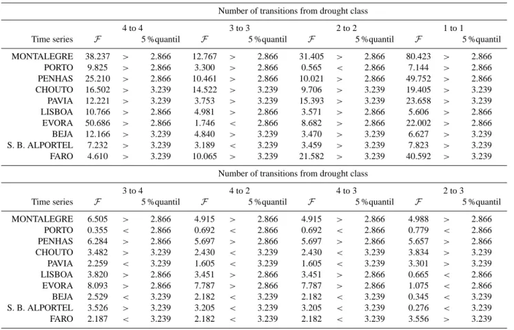
The F test with 5 % of significance level was applied to all drought class transitions. Results for the transitions that show significant differences among sub-periods are presented in Table 4. The other transitions not presented in Table 4 do not show significant differences among sub-periods for any lo-cation. This Table presents, for each location, the value of the F statistic and the 5 % quantil for the F distribution with 4 and 20 degrees of freedom in case of time series subdi-vided into 5 sub-periods, or with 3 and 16 degrees of free-dom for sub-periods. When the F statistic exceeds the 5 % quantil it can be concluded that there are significant differ-ences between the 5 or 4 sub-periods for that drought class transition and location. Results allow to conclude that, in general, there are significant differences between the 5 or 4 sub-periods of each time series for the transitions m4,4, m3,3, m2,2, m1,1, m3,4, m4,2, m4,3 and m2,3. Conversely, for the remaining transitions there were not significant differences. The transitions m1,1and m4,4have shown significant differ-ences among sub-periods, for all locations, whereas results for ´Evora and S. B. Alportel do not present significant differ-ences for m3,3. For the other transitions in Table 4 there are two or more locations not showing significant differences.
The number of transitions m1,1, m2,2, m3,3and m4,4, in-dicative of the maintenance in the same drought class, are of great importance for the analysis in the sense that they in-dicate the persistence of these drought classes. In particular, this is the case for m4,4, referring to the persistence of the severe/extreme drought class. Also highly important is m3,4,
Table 4. Results of the F test (> significant differences between sub-periods; < no significant differences between sub-periods). Number of transitions from drought class
4 to 4 3 to 3 2 to 2 1 to 1
Time series F 5 %quantil F 5 %quantil F 5 %quantil F 5 %quantil
MONTALEGRE 38.237 > 2.866 12.767 > 2.866 31.405 > 2.866 80.423 > 2.866 PORTO 9.825 > 2.866 3.300 > 2.866 0.565 < 2.866 7.144 > 2.866 PENHAS 25.210 > 2.866 10.461 > 2.866 10.021 > 2.866 49.752 > 2.866 CHOUTO 16.502 > 3.239 14.522 > 3.239 9.706 > 3.239 19.405 > 3.239 PAVIA 12.221 > 3.239 3.753 > 3.239 15.393 > 3.239 23.658 > 3.239 LISBOA 10.766 > 2.866 4.981 > 2.866 3.571 > 2.866 5.606 > 2.866 EVORA 50.686 > 2.866 1.746 < 2.866 8.682 > 2.866 22.002 > 2.866 BEJA 12.166 > 3.239 4.840 > 3.239 3.470 > 3.239 6.627 > 3.239 S. B. ALPORTEL 7.232 > 3.239 3.189 < 3.239 3.459 > 3.239 7.823 > 3.239 FARO 4.610 > 3.239 10.065 > 3.239 21.582 > 3.239 40.592 > 3.239
Number of transitions from drought class
3 to 4 4 to 2 4 to 3 2 to 3
Time series F 5 %quantil F 5 %quantil F 5 %quantil F 5 %quantil
MONTALEGRE 6.505 > 2.866 4.915 > 2.866 4.915 > 2.866 4.988 > 2.866 PORTO 0.355 < 2.866 0.692 < 2.866 0.692 < 2.866 0.779 < 2.866 PENHAS 6.284 > 2.866 5.697 > 2.866 5.697 > 2.866 5.657 > 2.866 CHOUTO 3.482 > 3.239 2.430 < 3.239 2.430 < 3.239 3.834 > 3.239 PAVIA 2.259 < 3.239 1.605 < 3.239 1.605 < 3.239 3.301 > 3.239 LISBOA 3.820 > 2.866 3.451 > 2.866 3.451 > 2.866 0.665 < 2.866 EVORA 8.093 > 2.866 7.787 > 2.866 7.787 > 2.866 1.075 < 2.866 BEJA 2.529 < 3.239 2.182 < 3.239 2.182 < 3.239 0.345 < 3.239 S. B. ALPORTEL 3.526 > 3.239 3.205 < 3.239 3.205 < 3.239 0.276 < 3.239 FARO 2.187 < 3.239 2.182 < 3.239 2.182 < 3.239 3.556 > 3.239
relative to the transition from moderate to the severe/extreme drought class, because this study aims to detect if droughts severity and frequency are increasing or not. The m3,3 and m4,3 deserve also particular attention because they refer re-spectively to the maintenance in the moderate drought class and to the transition from the severe/extreme to the moderate drought class.
Results indicating significant differences for the 5 % prob-ability level do not mean that there are significant differences between all sub-periods; hence, the Scheff´e multiple compar-ison method was applied to the cases where the frequencies have shown, for the F test, significant differences among sub-periods in order to find which pairs of sub-sub-periods actually have significant differences. Results of the Scheff´e multiple comparison are illustrated in Figs. 5 and 6.
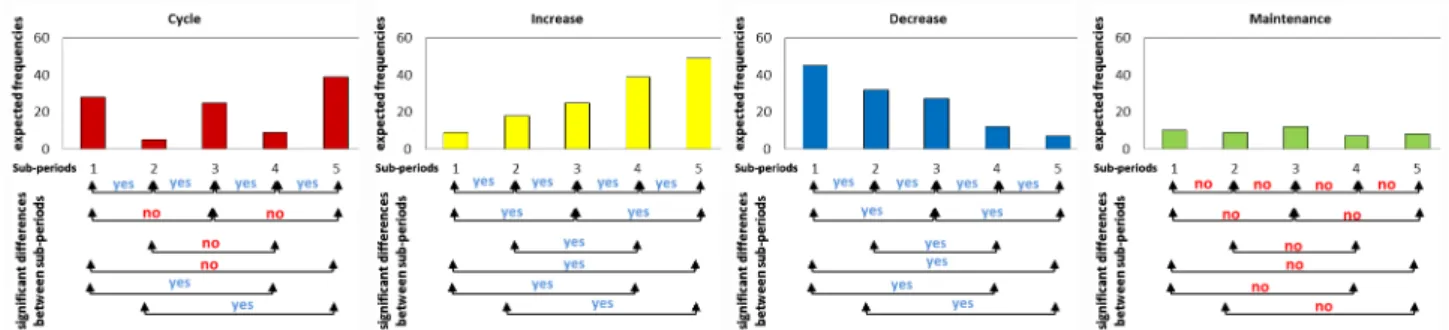
Figure 4 presents the pattern of what should be the typi-cal behaviour of a cycle of more or less severe droughts, in opposition to a trend of progressive drought increase during the last century, or a trend of progressive drought decrease as well as the case of maintenance of drought severity. In the case of cyclic behaviour, there is similarity between alternat-ing sub-periods and significant differences between consec-utive sub-periods. The difference between positive and neg-ative trends can only be detected through the observation of
the expected frequencies values. If they are increasing the trend is positive, otherwise it is negative (Fig. 4). Conversely, if there is a trend for drought aggravation or attenuation, lin-ear or non-linlin-ear, then significant differences must exist be-tween consecutive sub-periods. In case of maintenance, there is no significant differences between sub-periods. It must be noted that the conclusions about the behaviour of each loca-tion must have in consideraloca-tion both the results of the Scheff´e method and the graphical observation of the values of the expected frequencies, since the typical behaviours contem-plated in Fig. 4 may not be apparent.
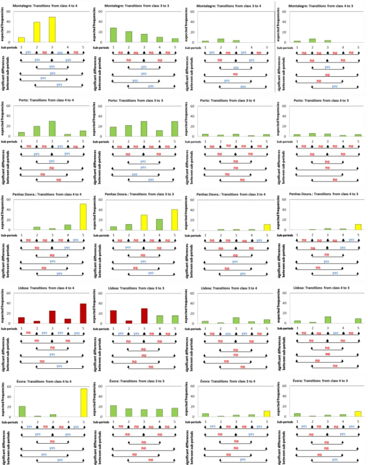
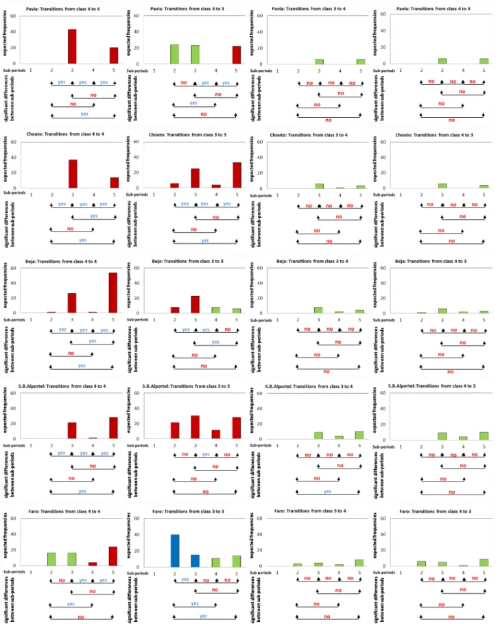
Figures 5 and 6 present the bar charts with the expected frequencies by sub-period for the number of transitions be-tween the drought classes of greater interest for this study, i.e. m4,4, m3,3, m3,4and m4,3. In these figures, color-coding is used in accordance to the typical behaviours described in Fig. 4: red when cycles are assumed, yellow when an increas-ing trend is detected, blue for decrease and green for persis-tence (nor trend or cycle). These colors are used in Fig. 1 to easy the locations of stations showing these behaviour as analysed in the following.
In the present study long time series were analysed. Three of them are from the northern Portugal and the others are from south. Analyzing the results of the first ones (Figs. 5 and
Fig. 4. Pattern charts and results for the Scheff´e multiple comparison method in the presence of a cyclic, upward trend, downward trend and maintenance behaviour. Arrows point to pairs of sub-periods being compared: “yes” when their differences are significant, “no” otherwise. In the case of trends: if the expected frequencies are increasing, the trend sign is positive; if the expected frequencies are decreasing, the trend sign is negative.
2), Montalegre presents a situation of increased occurrence of droughts from the 1st to the 3rd sub-period, a decrease from the 3rd to the 4th sub-period, and a maintenance from the 4th to the 5th. Overall, there is no evidence of drought aggravation for the period of 127 yr of observations. This be-haviour does not fit in any typical pattern and may relate to the fact that the local climate is humid, with the site elevation (1069 m) influencing the precipitation regime. Porto-Serra do Pilar (Figs. 5 and 2) also shows non-typical behaviour: dur-ing the first three sub-periods there is no evidence of changes in drought frequency and severity, while from the 3rd to the 4th sub-periods there is a significant decrease of droughts oc-currence and severity followed by a non-significant increase from the 4th to the 5th sub-periods. Thus, results do not show aggravation of drought for the last 135 yr but a possible at-tenuation. To be noted that Porto is near the Atlantic Ocean and has a sub-humid to humid climate. Both Montalegre and Porto are in Northern Portugal, a region that studies by San-tos et al. (2010), Sousa et al. (2011), or Vicente Serrano et al. (2011) identified as not subject to drought aggravation. The study by Paulo et al. (2012) using the MedPDSI has shown for Porto a significant trend for drought attenuation and for Montalegre a non-significant trend for attenuation.
Penhas Douradas (Figs. 5 and 2) shows a significant in-crease of the occurrence of severe/extreme droughts in the last sub-period in opposition to a maintenance of drought severity for the 4 antecedent sub-periods. Penhas Douradas has a humid climate and is located at 1380 m elevation; the significant increase in occurrence of severe/extreme droughts in the last 27 yr may be due to a variety of factors.
Lisboa (Figs. 6 and 3), if just considering the sub-periods 2, 3, 4 and 5, shows a typical cyclic behaviour, but this is not observed for the pair of the 1st and 2nd sub-periods. In fact, there is no evidence of significant decrease of severe/extreme droughts between sub-periods 1 and 2. Hence, results for Lisboa do not show any trend for increase or attenuation of droughts severity and frequency and in fact are more closer to a cycle. The application of the MK test to the MedPDSI
and to the SPEI indicated non-significant trends for respec-tively attenuation and aggravation of droughts (Paulo et al., 2012).
In the South (Figs. 6, 2 and 3) a more consistent cyclic behaviour could be found. Sites such as Pavia, Beja, Chouto and S. B. Alportel show a behaviour typical of a cycle with similarity between alternating sub-periods and significant differences between consecutive ones. The sub-periods with few severe/extreme droughts are followed by sub-periods of higher frequency and persistence of severe/extreme drought. Thus, results do not support the assumption of droughts ag-gravation or attenuation.
´
Evora (Figs. 6 and 3), in the middle of the drought vul-nerable Alentejo, seems to behave like an outlier in the sense that it would be expected that the sub-period 3 would have more severe/extreme droughts but, instead, this sub-period does not differ significatively from the 2nd and the 4th. The 1st sub-period shows to have a larger number of drought events, hence differing significatively from the fol-lowing sub-periods. However, the occurrence and severity of droughts also increase significantly in 5th sub-period rela-tive to the preceding ones, including relarela-tive to the first one. Therefore, this station does not show neither a clear long term trend for drought aggravation, or a cyclic behaviour; never-theless, droughts are aggravating in the last 27 yr of the con-sidered period of 135 yr. Using a shorter time span of only 65 yr, results of the MK test applied to the MedPDSI and the SPEI show a significant trend for aggravation. However, con-sidering the 135 yr data series and the results of the ANOVA-like inference test, it is not possible to affirm that droughts are aggravating at ´Evora.
Results for Faro (Figs. 6 and 3) have shown a signifi-cant increase in severe/extreme droughts when comparing the 4th and the 5th sub-periods, but not when comparing the other sub-periods and the 5th one. Thus, results for this loca-tion can not be interpreted as indicating a cyclic behaviour of droughts occurrence and severity, neither expressing a trend. Conversely, from the results of the previous study with
Fig. 5. Number of transitions between drought classes by sub-period and results for the Scheff´e multiple comparison of sub-periods. Arrows point to pairs of sub-periods being compared: “yes” when their differences are significant, “no” otherwise.
Fig. 6. Number of transitions between drought classes by sub-period and results for the Scheff´e multiple comparison of sub-periods. Arrows point to pairs of sub-periods being compared: “yes” when their differences are significant, “no” otherwise.
Appendix
Table A1 Estimates of QA log-linear model parameters fitted to contingency tables and correspondent residual deviances for the 10 sites by sub-period.
1st sub-period
Montalegre Porto Penhas Pavia Chouto Lisboa Evora´ Beja SBAlportel Faro
λ 1.008 1.361 0.785 1.974 1.337 λr2 −1.780 −2.350 −1.320 −2.518 −2.100 λr 3 −6.460 −7.680 −4.790 −7.970 −7.310 λr 4 −12.650 −14.770 −8.960 −13.630 −13.260 λc 2 −2.040 −2.400 −1.140 −2.564 −2.100 λc 3 −6.880 −7.810 −4.980 −8.120 −7.310 λc 4 −13.330 −14.890 −9.720 −13.760 −13.260 β 1.645 1.893 1.117 1.781 1.752 δ1 2.199 1.840 3.740 1.465 1.999 δ2 1.212 0.431 1.140 0.217 0.298 δ3 0.859 0.030 0.870 1.335 0.598 δ4 0.840 0.090 0.030 −0.594 0.201 G2 2.301 2.869 2.446 1.352 1.492 2nd sub−period
Montalegre Porto Penhas Pavia Chouto Lisboa ’Evora Beja SBAlportel Faro
λ 1.851 1.603 1.584 1.660 2.205 2.215 1.081 1.422 1.738 0.623 λr 2 −2.547 −2.033 −1.860 −1.450 −2.120 −2.550 −0.640 −0.430 −0.080 −0.726 λr3 −8.350 −7.670 −6.700 −7.160 −7.420 −8.170 −5.620 −5.300 −4.360 −5.570 λr4 −14.820 −13.820 −12.310 −13.410 −12.430 −14.380 −10.500 −9.280 −7.170 −10.440 λc2 −2.587 −2.032 −1.990 −1.480 −2.170 −2.590 −0.540 −0.510 −0.080 −0.789 λc3 −8.450 −7.720 −6.950 −7.170 −7.400 −8.400 −5.440 −5.540 −4.360 −5.670 λc4 −14.920 −14.050 −12.540 −14.120 −13.130 −14.980 −10.360 −10.110 −7.170 −10.680 β 1.947 1.794 1.506 1.601 1.494 1.786 1.240 1.082 0.819 1.422 δ1 0.865 1.400 2.198 1.169 1.471 1.135 2.690 2.608 2.362 1.945 δ2 0.140 −0.002 0.825 −0.036 0.937 0.460 −0.030 0.000 −0.069 0.360 δ3 0.473 0.731 0.997 1.440 0.960 0.078 1.594 1.772 2.661 1.514 δ4 0.396 0.561 0.960 0.250 −0.540 0.180 0.620 0.670 −0.510 0.521 G2 1.354 5.253 3.065 2.570 2.846 2.393 1.713 2.423 6.840 3.515 3tr sub−period
Montalegre Porto Penhas Pavia Chouto Lisboa ’Evora Beja SBAlportel Faro
λ 0.911 0.863 2.051 1.054 1.118 1.667 1.283 1.120 1.371 1.518 λr 2 −0.428 −0.804 −2.550 −1.400 −1.965 −2.056 −1.128 −1.076 −1.594 −2.490 λr 3 −3.920 −5.600 −8.110 −6.420 −6.680 −7.490 −5.110 −6.100 −6.670 −7.900 λr 4 −7.100 −9.610 −14.580 −11.680 −12.190 −11.810 −10.320 −9.860 −10.420 −14.960 λc 2 −0.428 −0.867 −2.600 −1.457 −2.048 −2.056 −1.192 −1.131 −1.652 −2.540 λc3 −3.920 −5.740 −8.260 −6.590 −6.860 −7.490 −5.170 −6.230 −6.810 −8.030 λc4 −7.100 −9.720 −14.710 −11.980 −12.350 −11.810 −10.380 −9.960 −10.540 −15.080 β 0.958 1.340 1.808 1.574 1.643 1.680 1.275 1.408 1.512 1.914 δ1 2.849 2.731 1.185 2.328 2.375 1.505 2.678 2.462 2.036 1.611 δ2 0.954 −0.020 0.523 −0.121 0.614 0.191 0.389 −0.070 0.389 0.507 δ3 1.080 1.814 1.446 0.925 0.858 1.594 0.148 1.662 1.895 −0.109 δ4 1.837 0.425 −0.590 1.182 0.744 −1.708 0.624 −0.572 −1.570 0.667 G2 0.430 1.457 2.979 5.938 1.341 1.958 0.080 2.500 2.479 2.872 4th sub−period
Montalegre Porto Penhas Pavia Chouto Lisboa ’Evora Beja SBAlportel Faro
λ 2.246 1.322 0.421 3.023 2.256 0.987 0.990 1.617 1.345 0.706 λr 2 −2.290 −1.770 −0.960 −3.150 −2.310 −0.953 −1.592 −0.966 −2.400 −0.575 λr 3 −7.230 −6.600 −5.630 −8.140 −7.200 −5.090 −6.280 −4.680 −7.260 −4.550 λr 4 −12.110 −12.730 −12.120 −12.550 −11.530 −8.330 −11.590 −9.000 −13.510 −7.810 λc 2 −2.330 −1.990 −1.040 −3.190 −2.370 −1.030 −1.592 −0.966 −2.400 −0.575 λc 3 −7.630 −6.830 −5.800 −8.790 −7.170 −5.550 −6.280 −4.680 −7.350 −4.550 λc 4 −13.080 −12.560 −12.680 −13.700 −12.220 −8.850 −11.590 −9.000 −13.810 −7.810 β 1.478 1.560 1.531 1.545 1.396 1.154 1.522 1.056 1.750 1.006 δ1 1.780 2.392 3.097 0.840 1.830 3.116 2.786 2.665 2.252 3.765 δ2 0.576 0.829 0.116 1.677 1.209 1.044 0.615 0.485 0.949 0.685 δ3 1.610 0.561 0.328 0.000 0.940 2.036 0.576 0.319 −0.091 1.733 δ4 −0.710 0.400 2.180 −1.500 −0.840 −0.070 −2.160 −0.520 −2.020 0.210 G2 2.179 2.416 2.461 2.017 3.143 8.857 1.528 9.058 2.742 2.733 5th sub−period
Montalegre Porto Penhas Pavia Chouto Lisboa ’Evora Beja SBAlportel Faro
λ 1.605 2.299 1.134 2.030 1.655 1.481 1.105 1.578 1.926 2.579 λr2 −1.620 −3.110 −2.830 −3.080 −2.510 −1.434 −1.466 −1.142 −2.632 −2.939 λr3 −6.510 −9.010 −8.250 −8.710 −8.140 −6.760 −6.380 −6.380 −7.000 −7.370 λr4 −11.810 −15.940 −16.160 −15.680 −15.220 −10.210 −10.440 −9.740 −12.770 −11.700 λc 2 −1.670 −3.120 −2.820 −3.030 −2.510 −1.436 −1.532 −1.142 −2.567 −2.886 λc 3 −6.770 −8.920 −8.300 −8.670 −8.200 −6.710 −6.520 −6.380 −6.940 −7.180 λc 4 −12.700 −15.640 −16.200 −15.460 −15.490 −10.100 −10.560 −9.740 −12.710 −11.530 β 1.437 1.986 2.147 1.987 1.937 1.463 1.517 1.316 1.674 1.538 δ1 2.342 0.664 0.796 1.059 1.244 2.005 2.097 1.988 1.424 1.025 δ2 0.428 0.620 0.716 0.641 0.296 −0.055 0.422 −0.016 0.922 1.562 δ3 0.690 1.151 −0.197 0.568 0.741 1.599 0.982 1.128 0.282 0.769 δ4 −0.090 −0.100 0.811 0.321 0.700 −0.909 −0.344 0.821 0.103 −0.774 G2 2.265 2.715 2.861 3.401 2.706 2.089 1.714 1.947 3.300 4.018
shorter time series with 67 yr applied to the Alentejo re-gion only (Moreira et al., 2006), a marked spatial variation is apparent in the present study.
For the northern part of the country, where locations have a humid climate and data sets are longer than 127 yr, the cyclic behaviour was not found. Porto and Montalegre also do not show trends for droughts aggravation but Penhas Douradas shows an aggravation of droughts for the last sub-period. For the South, cases of Lisboa, Pavia, Chouto, Beja and S. B. Al-portel, results show a behaviour generally consistent with a cyclic occurrence and severity of droughts. Conversely,
´
Evora and Faro show a significant aggravation of droughts for the 5th period only; however, because these results are in contradiction with those of other locations within the same region, it is not possible to relate the identified aggravation of droughts with climate change but with spatial variability as referred for other regions. Hence, there is a possibility that droughts behaviour in the Alentejo region may be due to long-term natural variability.
5 Conclusions
ANOVA-like inference together with log-linear models have shown high potential to compare drought class transitions among different sub-periods. The methodology revealed to be robust and very sensitive in detecting variability. In this study, ANOVA is a new approach that can be used as an al-ternative to the odds ratios and correspondent confidence in-tervals, as used in a former analysis with log-linear models. It allows not only to perceive if droughts are or not aggravating but the dynamics of changes from one sub-period to another. The method allows also to perceive differences in drought dynamics from one location to another. These aspects are ad-vantageous relative to just use a trend test.
In southern Portugal, results for the sites of Pavia, Beja, Chouto, S. B. Alportel and Lisboa have shown that droughts occurrence and severity behave in a cyclic way, in which a sub-period with few severe/extreme droughts is followed by a sub-period where severe/extreme droughts are frequent. This cycle may be related to a long-term natural variability, with the duration of the sub-periods ranging from 26 to 30 yr. For the other locations, mainly those from the North, there is no evidence of a typical cyclic behaviour neither a trend for drought aggravation. Therefore, globally, the results do not support the assumption of a trend of drought aggravation since the beginning of the twenty century that could be re-lated to climate change. Nevertheless, if comparing the last period of 27 yr with the precedent one of 24, there is gener-ally a significant increase of droughts occurrence and sever-ity with exception of Montalegre and Porto in the northern re-gion. Results also confirm the need for using long time series and show a strong influence of spatial variability.
Acknowledgements. This work was partially supported by the research project PTDC/AGR-AAM/71649/2006 – Droughts Risk Management: Identification, Monitoring, Characterization, Prediction and Mitigation as well as by CMA/FCT/UNL under the project PEst-OE/MAT/UI0297/2011.
Edited by: B. van den Hurk
References
Agresti, A.: Categorical Data Analysis, J. Wiley& Sons, New York, 1990.
Alcoforado, M. J., Nunes, M. F., Garcia, J. C., and Taborda, J. P.: Temperature and precipitation reconstruction in southern Portu-gal during the late Maunder Minimum (AD 1675–1715), The Holocene 10, 333–340, 2000.
Beniston, M., Stephenson, D. B., Christensen, O. B., Ferro, C. A. T., Frei, C., Goyette S., Halsnaes, K., Holt, T., Jylh¨a, K., Koffi, B., Palutikof, J., Sch¨oll, R., Semmler, T., and Woth, K.: Future extreme events in European climate: an exploration of regional climate model projections, Climatic Change, 81, 71–95, 2007. Bonaccorso, B., Bordi, I., Cancelliere A., Rossi G., and Sutera, A.:
Spatial variability of drought: an analysis of the SPI in Sicily, Water Resour. Manage., 17, 273–296, 2003.
Bordi, I., Fraedrich, K., Jiang, J.-M., and Sutera, A.: Spatio-temporal variability of dry and wet periods in eastern China, The-oretical Applied Climatology, 79, 81–91, 2004.
Bordi, I., Fraedrich, K., Petitta, M., and Sutera, A.: Large-scale assessment of drought variability based on NCEP/NCAR and ERA-40 re-analyses, Water Resour. Manage., 20, 899–915, 2006.
Bordi, I., Fraedrich, K., Petitta M., and Sutera. A.: Extreme value analysis of wet and dry periods in Sicily, Theorectical and Aplied Climatology, 87, 61–71, 2007.
Bordi, I., Fraedrich, K., and Sutera, A.: Observed drought and wet-ness trends in Europe: an update, Hydrol. Earth Syst. Sci., 13, 1519–1530, doi:10.5194/hess-13-1519-2009, 2009.
Burke, E. J., Brown, S. J., and Christidis, N.: Modeling the Recent Evolution of Global Drought and Projections for the Twenty-First Century with the Hadley Centre Climate Model, J. Hydrom-eteorol., 7, 1113–1125, 2006.
Dai, A.: Characteristics and trends in various forms of the Palmer Drought Severity Index during 1900-2008, J. Geophis. Res., 116, D12115, doi:10.1029/2010JD015541, 2011.
Dai, A., Trenberth, K. E., and Qian, T.: A global dataset of Palmer Drought Severity Index for 1870-2002: Relationship with soil moisture and effects of surface warming, J. Hydrometeorol., 5, 1117–1130, 2004.
Dracup, J. A., Lee, K. S., and Paulson, E. G.: On the definition of droughts, Water Resour. Res., 16, 297–302, 1980.
Heim Jr., R. R.: A review of Twentieth-Century drought indices used in the United States, B. Am. Meteorol. Soc., 83, 1149–1165, 2002.
Heinrich, G. and Gobiet, A.: The future of dry and wet spells in Europe: A comprehensive study based on the ENSEM-BLES regional climate models, Int. J. Climatol., in press, doi:10.1002/joc.2421, 2011.
Helsel, D. R. and Hirsch, R. M.: Statistical Methods in Water Re-sources, Elsevier, Amsterdam, 1992.
Hocking, R.: Methods and Applications of Linear Models, John Willey & Sons, New York, 2003.
Huntington, T. G.: Evidence for intensification of the global water cycle: Review and synthesis, J. Hydrol., 319, 83–95, 2006. Katz, R. W., Parlange, M. B., and Naveau, P.: Statistics of extremes
in hydrology, Adv. Water Resour., 25, 1287–1304, 2002. Keyantash, J. and Dracup, J. A.: The quantification of drought: An
evaluation of drought indices, B. Am. Meteorol. Soc., 83, 1167– 1180, 2002.
Lehner, B., D¨oll, P., Alcamo, J., Henrichs, T., and Kaspar, F.: Esti-mating the impact of global change on flood and drought risks in Europe: A continental, integrated analysis, Climatic Change, 75, 273–299, 2006.
Lehmann, E.: Testing Statistical Hypotheses, Springer, New York, 1997.
Lloyd-Hughes, B.: A spatio-temporal structure-based approach to drought characterisation, Int. J. Climatol., 32, 406–418, 2012. Lloyd-Hughes, B. and Saunders M. A.: A drought climatology for
Europe, Int. J. Climatol., 22, 1571–1592, doi:10.1002/joc.846, 2002.
Ito, K.: Robusteness of ANOVA and MANOVA test procedures, edited by: Krishnaiah, P. R., Handbook of Statistics, Vol. 1, North-Holland Publishing Company, 199–236, 1980.
Martins, D. S., Raziei, T., Paulo, A. A., and Pereira, L. S.: Spatial and temporal variability of precipitation and drought in Portugal, Nat. Hazards Earth Syst. Sci., 12, 1493–1501, doi:10.5194/nhess-12-1493-2012, 2012.
Mazvimavi, D.: Investigating changes over time of annual rain-fall in Zimbabwe, Hydrol. Earth Syst. Sci., 14, 2671–2679, doi:10.5194/hess-14-2671-2010, 2010.
McKee, T. B, Doesken, N. J., and Kleist, J.: The relationship of drought frequency and duration to time scales, in: 8th Conference on Applied Climatology, Am. Meteor. Soc., Boston, 179–184, 1993.
McKee, T. B., Doesken, N. J., and Kleist, J.: Drought monitoring with multiple time scales. In: 9th Conference on Applied Clima-tology, Am. Meteor. Soc., Boston, 233–236, 1995.
Mishra, A. K. and Singh, V. P.: A review of drought concepts, J. Hydrol., 391, 202–216, 2010.
Mishra, A. K., Singh, V. P., and Desai, V. R.: Drought characteriza-tion: a probabilistic approach, Stoch. Environ. Res. Risk Assess., 23, 41–55, 2009.
Montgomery, D. C.: Design and Analysis of Experiments – 5th Edn., John Willey & Sons, New York, 1997.
Moreira, E. E., Paulo, A. A., Pereira, L. S., and Mexia, J. T.: Anal-ysis of SPI drought class transitions using loglinear models, J. Hydrol., 331, 349–359, 2006.
Moreira, E. E., Coelho, C. A., Paulo, A. A., Pereira, L. S., and Mexia, J. T.: SPI-based drought category prediction using log-linear models, J. Hydrol., 354, 116–130, 2008a.
Moreira, E. E., Pereira, L. S., and Mexia, J. T.: Assessing cycles of severe/extreme drought events using spectral analysis of precip-itation time series in: New Topics in Water Resources Research and Management, Novapublishers, New York, 349–362, 2008b. Nelder, J. A.: Loglinear models for contingency tables: a
general-ization of classical least squares, Appl. Statistics, 23, 323–329, 1974.
Nicault, A., Alleaume, S., Brewer, S., Carrer, M., Nola, P., and Guiot, J.: Mediterranean drought fluctuation during the last 500
years based on tree-ring data, Clim. Dynam., 31, 227–245, doi:10.1007/s00382-007-0349-3, 2008.
Palmer, W.C.: Meteorological drought, Research Paper No. 45, US Weather Bureau, 1965.
Paulo, A. A. and Pereira, L. S.: Drought concepts and characteri-zation: comparing drought indices applied at local and regional scales, Water Int., 31, 37–49, 2006.
Paulo, A. A. and Pereira L. S.: Prediction of SPI drought class tran-sitions using Markov chains, Water Resour. Manage., 21, 1813– 1827, 2007.
Paulo, A. A. Pereira, L. S.: Stochastic prediction of drought class transitions, Water Resour. Manage., 22, 1277–1296, 2008. Paulo, A. A., Pereira, L. S., and Matias, P. G.: Analysis of local and
regional droughts in southern Portugal using the theory of runs and the Standardized Precipitation Index, in: Tools for Drought Mitigation in Mediterranean Regions, edited by: Rossi, G., Can-celliere, A., Pereira, L. S., Oweis, T., Shatanawi, M., and Zairi, A., Dordrecht, Kluwer, 55–78, 2003.
Paulo, A. A., Ferreira, E., Coelho, C., and Pereira, L. S.: Drought class transition analysis through Markov and Loglinear models, an approach to early warning. Agric. Water Manage, 77, 59–81, 2005.
Paulo, A. A., Rosa, R. D., and Pereira, L. S.: Climate trends and be-haviour of drought indices based on precipitation and evapotran-spiration in Portugal, Nat. Hazards Earth Syst. Sci., 12, 1481– 1491, doi:10.5194/nhess-12-1481-2012, 2012.
Pereira, L. S., Rosa, R. D., and Paulo, A. A.: Testing a modifi-cation of the Palmer drought severity index for Mediterranean environments, in: Methods and Tools for Drought Analysis and Management, edited by: Rossi, G., Vega, T., and Bonaccorso, B., Springer, Dordrecht, 149–167, 2007.
Pereira, L. S., Cordery, I., and Iacovides, I.: Coping with Water Scarcity, Addressing the Challenges, Springer, Dordrecht, 2009. Piccarreta, M., Capolongo, D., and Boenzi, F.: Trend analysis of precipitation and drought in Basilicata from 1923 to 2000 within a southern Italy context, Int. J. Climatol., 24, 907–922, 2004. Raziei, T., Bahram, S., Paulo, A., Pereira, L., and Bordi, I.: Spatial
Patterns and Temporal Variability of Drought in Western Iran, Water Resour. Manage., 23, 439–455, 2009.
Reiser, H. and Kutiel, H.: Rainfall uncertainty in the Mediterranean: time series, uncertainty, and extreme events, Theor. Appl. Clima-tol., 104, 357–375, 2011.
Rodrigo, F. S., Esteban-Parra, M. J., Pozo-V´azques, D., and Castro-D´ıez, Y.: Rainfall variability in souther Spain on decadal to cen-tennial time scales, Int. J. Climatol., 20, 721–732, 2000. Ruiz Sinoga, J. D. and Gross, T. L.: Droughts and their social
per-ception in the mass media (southern Spain), Int. J. Climatol., in press, doi:10.1002/joc.3465, 2012.
Santos, J. F., Pulido-Calvo, I., and Portela, M.: Spatial and tempo-ral variability of droughts in Portugal, Water Resour. Res., 46, W03503, doi:10.1029/2009WR008071, 2010.
Scheff´e, H.: The Analysis of Variance, John Willey & Sons, New York, 1959.
Shang, H., Yan, J., Gebremichael, M., and Ayalew, S. M.: Trend analysis of extreme precipitation in the Northwestern High-lands of Ethiopia with a case study of Debre Markos, Hy-drol. Earth Syst. Sci., 15, 1937–1944, doi:10.5194/hess-15-1937-2011, 2011.
Shao, Q. and Li, M.: A new trend analysis for seasonal time series with consideration of data dependence, J. Hydrol., 396, 104–112, 2011.
Sousa, P. M., Trigo, R. M., Aizpurua, P., Nieto, R., Gimeno, L., and Garcia-Herrera, R.: Trends and extremes of drought indices throughout the 20th century in the Mediterranean, Nat. Haz-ards Earth Syst. Sci., 11, 33–51, doi:10.5194/nhess-11-33-2011, 2011.
Steinemann, A. C., Hayes, M. J., and Cavalcanti, L. F. N.: Drought Indicator and Triggers, in: Drought and Water Crises, edited by: Wilhite, D. A., Taylor and Francis Group, New York, 2005. Suhailaa, J., Jemainb, A. A., Hamdana, M. F., and Zinb, Z.
W.: Comparing rainfall patterns between regions in Peninsular Malaysia via a functional data analysis technique, J. Hydrol., 411, 197–206, 2011.
Tate, E. L. and Gustard, A.: Drought definition: a hydrological per-spective, in: Drought and Drought Mitigation in Europe, edited by: Vogt, J. V. and Somma, F., Kluwer Academic Publishers, The Netherlands, 23–48, 2000.
Vicente-Serrano, S. M.: Differences in Spatial Patterns of Drought on Different Time Scales: An Analysis of the Iberian Peninsula, Water Resour. Manage., 20, 37–60, 2006.
Vicente-Serrano, S. M. and Cuadrat-Prats, J. M.: Trends in drought intensity and variability in the middle Ebro valley (NE of the Iberian peninsula) during the second half of the twentieth cen-tury, Theor. Appl. Climatol., 88, 247–258, 2007.
Vicente-Serrano, S.M., L´opez-Moreno, J.I., Drumond, A., Gimeno, L., Nieto, R., Mor´an-Tejeda, E., Lorenzo-Lacruz, J., Beguer´ıa, S., and Zabalza, J.: Effects of warming processes on droughts and water resources in the NW Iberian Peninsula (1930–2006), Clim. Res., 48, 203–212, 2011.
Wilhite, D. A. Buchanan-Smith, M.: Drought as Hazard: Under-standing the Natural and Social Context, in: Drought and Water Crises, edited by: Wilhite, D. A., Taylor and Francis Group, New York, 2005.