Best practice of risk modelling in motor insurance : using GLM and Machine Learning approach

(1)

Master in

Actuarial Science

Master’s Final Work

Internship Report

Best Practice of Risk Modelling in Motor Insurance - Using GLM and

Machine Learning Approach

Xu Zhifeng

Faculty Advisor: João Manuel de Sousa Andrade e Silva

Industry Supervisor: Clayton Chiong

(2)

Acknowledgements

Professor João Andrade e Silva from ISEG guided through my work carefully with pa-tience. He is knowledgeable and kind. It is my honor that he supervised my master’s final work. His feedback is really important for my work. Besides, he had given me a lot of help during my entire master’s study, including the supervision of our Society of Actuaries case study challenge, and coursework study of Risk Models. I truly appreciate all these kind helps and guidance very much.

I would like to give huge thanks to my industry supervisor Clayton Chiong, who is a true professional of the risk modelling area in actuarial works, he also has exposure to various areas related. Clayton kept giving me quick and instructive response whenever I encounter a problem. He is a passionate person and played a key role in this project. Thanks Ana-Luzia Soares from local pricing team, who helped me a lot in terms of understanding the Portuguese auto insurance book structure and SAS projects, when I entered the company, her help made me feel warm in the working environment.

Drishti Singhvi worked together with me closely during the machine learning phase, she is creative and a quick learner, result from her help I have a better understanding of the methodologies we are using, and gain knowledge from other experienced data scientists in the company.

Samuel Vandello is really helpful in terms of building the GLM models and make connec-tion between machine learning outcome and tradiconnec-tional GLM. He managed to organize our GLM works together as a team, and also helped consulting author of the internal package for the technical questions.

Also many thanks to Professor Maria de Lourdes Centeno, who connected ISEG with Liberty.

Finally, I would like to give a big hug to my parents, who always support me in the back and never question my choice in the life.

(3)

Abstract

Insurance pricing nowadays is getting more and more interesting and challenging due to the fact that the dimension of analysable data is evolutionarily exploding. It is an urgent call for insurers to reconsider how to deal with the data more accurately and precisely. To implement pricing sophistication in motor insurance products, we apply cutting edge machine learning techniques including penalized GLM and boosting methods, which help us identify the important features among massive amount of candidate variables, and detect potential interactions without trying the endless two-way combinations manually. In order to sufficiently make use of these methods, we need to deeply understand the research objective, preliminary assumptions and statistical backgrounds.

Although there is some evidence indicating the existence of higher predictive power of machine learning models compared with traditional GLM (Generalized Linear Models), GLM is more convenient and interpretable, especially for multiplicative models. GLM model is easier to be demonstrated to stakeholder, therefore we still achieve our risk models in GLM, but absorbing the insights from our machine learning results.

The evaluation of models is done by progression, it is generally performed by residual analysis of the training or validation dataset, and testing errors for the holdout dataset. After peer review, we apply some adjustment in each model, to get models that are significant and robust. They are expected to have high predictive power in the out-of-sample data, thus can be used in the future.

Keywords: motor insurance, machine learning, pricing sophistication, penalized GLM, boosting, GLM, residual analysis, training, validation, holdout

(4)

Resumo

O pricing na atividade seguradora está a tornar-se cada vez mais interessante e desafi-ador pelo facto de a dimensão dos dados a analisar estar a crescer de forma explosiva. Torna-se assim urgente para as seguradoras reconsiderar a forma de lidar com este vol-ume de dados.

Para implementar modelos sofisticados de pricing para produtos de seguro automóvel, aplicámos técnicas de machine learning, incluindo modelos GLM penalizados e métodos de boosting, que ajudam a identificar as características mais importantes de entre uma grande quantidade de variáveis candidatas. Estes métodos também permitem detetar potenciais interações sem testar as inúmeras combinações bidimensionais. Para um uso eficiente desses métodos, é necessário compreender o objetivo do modelo, as hipóteses que o suportam e dominar as metodologias estatísticas.

Embora haja alguma evidência de um maior poder preditivo dos modelos baseados em machine learning quando comparados com os tradicionais GLM (Modelos Lineares Gen-eralizados), estes últimos beneficiam de uma estrutura (especialmente para modelos mul-tiplicativos), mais conveniente e mais interpretável. O modelo GLM é mais fácil de ex-plicar às partes interessadas o que nos levou a utilizar os GLM na modelação do risco, mas absorvendo os ensinamentos dados pelos modelos de machine learning.

A avaliação dos modelos é realizada pela análise dos resíduos quer na fase de treino quer de validação quer ainda de teste.

Após a revisão pela equipa, aplicam-se alguns ajustes em cada modelo para reforçar a sua significância e a sua robustez. Espera-se que eles tenham alto poder preditivo nos dados fora da amostra e possam, portanto, ser usados no futuro.

Palavras-chave: seguro automóvel, machine learning, modelos sofisticação de pric-, modelos GLM penalizadospric-, boostingpric-, GLMpric-, análise dos resíduospric-, treinopric-, validaçãopric-,

(5)

List of Figures

3.1 Ridge and LASSO constrain surface for 3 element β vector . . . 12 3.2 Estimation of β shrinkage path among different α . . . 15 3.3 Gamma loss on cross validation dataset for theft severity peril . . . 15 3.4 Ranking of average estimated beta by cross validation of the theft severity

model . . . 16 3.5 Rescaled frequency average graph by variable driver age for theft peril . . 20 3.6 Validation error iteration of different parameters of third party liability

(property damage) severity model . . . 22 4.1 Adding interaction effect to two continuous variables in the linear predictor 29 4.2 Residual of RCM severity model . . . 31 5.1 Gamma fit test of windscreen severity . . . 34 5.2 Gamma fit test of windscreen excess loss severity . . . 35

(8)

List of Tables

2.1 List of coverage abbreviations with description . . . 3

2.2 Bonus-Malus levels for TPL coverage based on no-claim years . . . 6

2.3 Transition rules for TPL Bonus-Malus levels . . . 6

3.1 Dummy columns for categorical variable . . . 13

3.2 Feature importance ranking result. . . 17

3.3 Potential interactions ranking result. . . 22

3.4 Pre-testing of interactions . . . 24

(9)

Chapter 1 Introduction

This is a technical report of the internship work at Liberty Seguros®1 _{dedicated in the}

“Portugal Auto Risk Modelling Project” during March 2020 to July 2020, at Liberty Mu-tual Insurance Western European Market. This exciting high profile project consists of different sub tasks, including data preparation, deciding risk modelling approach, build-ing risk technical model, etc.

1.1 Motivation

This project is aimed at performing the best practice of pricing analysis, with the ambi-tious goal of transforming how pricing is done in WEM2 _{by implementing cutting edge}

pricing models, leading to unlock the profit potential on WEM accounts.

1.2 Objectives

The mains tasks of this project are:

• Incorporate best practice pricing and machine learning techniques, develop best in class risk models collaborating with actuaries and data scientists across WEM, US and global teams.

1_{Branch of Liberty Mutual Insurance in Portugal.} 2_{Western European Market}

(10)

Xu Zhifeng CHAPTER 1. INTRODUCTION

• Work closely with key stakeholders in the business to deliver the optimal rates for each distribution channel.

To be more specific, in the first 1.5 to 2 months, the task is to learn about the Portuguese auto insurance business, investigate existing modelling SAS project and update datasets, assist claims analysis to inform modelling strategy, data reconciliation, data enrichment from external sources, preliminary feature engineering, process data and create files for statistical softwares. The data enrichment and process part is continuously progressing according to our modelling requirements.

In the following 2 months, the main task is to build machine learning model to detect potential important features and interactions. At the same time model frequency and severity for different perils as a team in GLM.

The last 2 months is for the technical model collaboration of GLM and machine learning results, preparing impact analysis and proposal presentation to stakeholders.

1.3 Structure

Chapter 2 is the summary of Liberty’s main product’s coverage, and some essential information of our data. The core methodology and practice procedure of machine learning can be found in chapter 3. In this chapter we use machine learning to do features and interactions selection, root in penalized GLM and extreme gradient boosting. The sound background of GLM models is in chapter 4, including detail of the general models and complex components. Following chapter 5 is for the technical model collaboration procedure, for perils separate frequency and severity models, we combine them in this chapter, for perils models as a whole, we address the final modelling decision before restricted models. The last chapter is the conclusion of this project.

(11)

Chapter 2 Book Structure and Data

There are various products under auto insurance sector of Liberty Seguros, “Liberty So-bre Rodas” [LibertySeguros, 2019b] and “Liberty 2 Rodas”[LibertySeguros, 2019a] have the biggest market share. Here we introduce the product book structure of Liberty by referencing general and special conditions in product “Liberty Sobre Rodas”.

2.1 Coverage

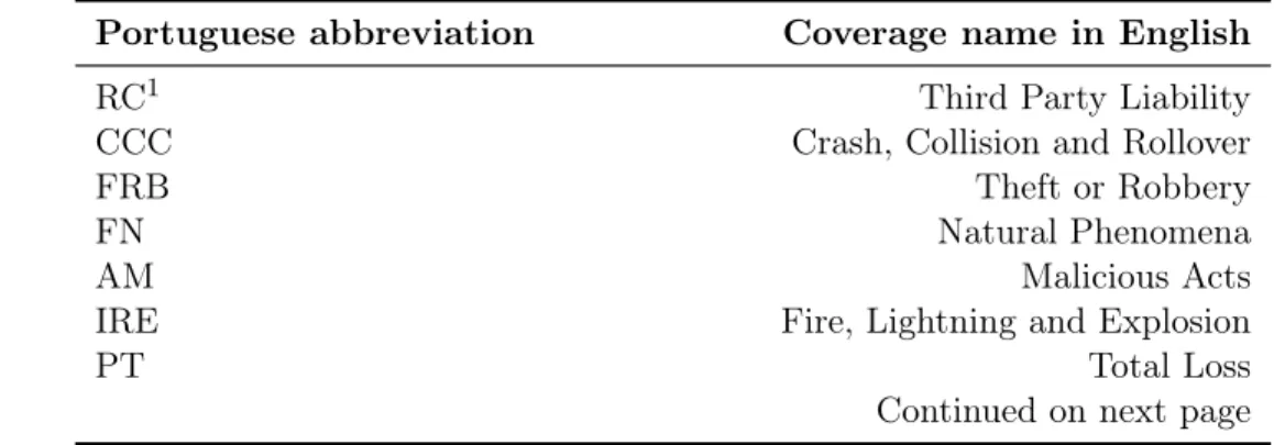
In table 2.1 we have the abbreviation of coverage (cobertura in Portuguese), and the English coverage names of them. Under each coverage, there are one or several covers (garantias in Portuguese). The covers information can be found in appendix A.

Table 2.1: List of coverage abbreviations with description

Portuguese abbreviation Coverage name in English

RC1 Third Party Liability

CCC Crash, Collision and Rollover

FRB Theft or Robbery

FN Natural Phenomena

AM Malicious Acts

IRE Fire, Lightning and Explosion

PT Total Loss

Continued on next page

(12)

Xu Zhifeng CHAPTER 2. BOOK STRUCTURE AND DATA

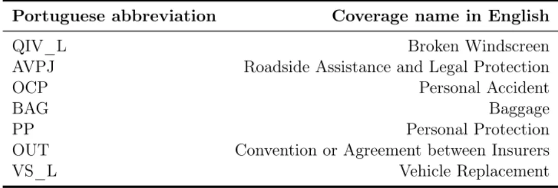
Table 2.1 – continued from previous page

Portuguese abbreviation Coverage name in English

QIV_L Broken Windscreen

AVPJ Roadside Assistance and Legal Protection

OCP Personal Accident

BAG Baggage

PP Personal Protection

OUT Convention or Agreement between Insurers

VS_L Vehicle Replacement

2.1.1 Main Covers

The perils we modelled in our GLM are considered as main covers. We choose the perils by the aggregate loss. The five perils we chose add up to more than 95 % of loss in the past 5 years.

Third Party Liability Property Damage

Losses ensuing from damage or injury to movable or immovable property or animals who, as a result of an incident covered by this contract, suffers damage or injury that entitles them to compensation or indemnification under the terms of civil law and this policy. Third Party Liability Personal Injury

Losses ensuing from injury to physical or mental health for anyone who, as a result of an incident covered by this contract, suffers damage or injury that entitles them to compensation or indemnification under the terms of civil law and this policy.

Crash, Collision and Rollover

The following definitions apply for the purposes of this cover: Collision: when the vehicle strikes any other object in motion;

Crash: when the vehicle strikes any other stationary object or the vehicle is struck while stationary;

(13)

Rollover: when the vehicle is no longer in its normal position, but not as the result of a crash or collision.

Broken Windscreen

Through this Special Condition, Liberty Seguros covers the cost of repairs or replacement of damage resulting from broken glass, or the equivalent in synthetic material, in the windscreen, the rear window, the sunroof, the side windows or the panoramic sunroof. Theft or Robbery

When this Special Condition is contracted, Liberty Seguros covers the cost of damage to the insured vehicle, where this ensues from the disappearance, destruction or deteri-oration of the same due to attempted or actual theft, robbery or unauthorised use. Disappearance of the vehicle;

Theft of parts, devices, accessories or instruments; Damage in the event of attempted theft or robbery; Replacement of keys and substitution of lock.

2.1.2 Non-Main Covers

For the remaining covers, we use one-way or two-way table to analysis their loss be-haviour, without putting into GLM or machine learning models.

2.2 Bonus-Malus

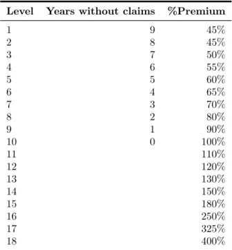
We use NCD (No Claim Discount) system to implement the Bonus-Malus of auto insur-ance premium. Since we have different coverage insured, there are 2 different tables of Bonus-Malus applying for Third-Party Liability (marked as TPL) and Collision damage (Crash, Collision, Rollover, Fire, Lightning Strike and Explosion and Acts of Vandalism). Here we use TPL Bonus-Malus table for policyholder with one vehicle that joined Liberty without previous insured history (started from 100%) as an example. The percentage premium and transition rule matrix can be found in the tables below.

(14)

Table 2.2: Bonus-Malus levels for TPL coverage based on no-claim years

Level Years without claims %Premium

1 9 45% 2 8 45% 3 7 50% 4 6 55% 5 5 60% 6 4 65% 7 3 70% 8 2 80% 9 1 90% 10 0 100% 11 110% 12 120% 13 130% 14 150% 15 180% 16 250% 17 325% 18 400%

Table 2.3: Transition rules for TPL Bonus-Malus levels

Next level if # claims in the year Current level 0 1 2 3 4 5 6+ 1 1 4 7 10 13 16 18 2 1 5 8 11 14 17 18 3 2 6 9 12 15 18 18 4 3 7 10 13 16 18 18 5 4 8 11 14 17 18 18 6 5 9 12 15 18 18 18 7 6 10 13 16 18 18 18 8 7 11 14 17 18 18 18 9 8 12 15 18 18 18 18 10 9 13 16 18 18 18 18 11 10 14 17 18 18 18 18 12 11 15 18 18 18 18 18 13 12 16 18 18 18 18 18 14 13 17 18 18 18 18 18 15 14 18 18 18 18 18 18 16 15 18 18 18 18 18 18 17 16 18 18 18 18 18 18 18 17 18 18 18 18 18 18

(15)

2.3 Data and Software

The dataset is pre-processed in SAS® _{Enterprise Guide}® _software2_{, the main format}

used for SAS data is .sas7bat file. We build our GLM models in Emblem®3_{, which use}

.bid and .fac format data, so we convert our .sas7bdat data into .bid and .fac format. For machine learning, we use RStudio®4_.

The data can be separated by individual and company, or private and commercial. At this stage we focus on the building tariff for individual and private policies. Our data is aggreagated from different platforms and different sources. The data column cate-gories include time (TI), model control (ADM), driver information (DR), policy infor-mation (SA), vehicle (VH), geographical (GEO), claim experience (CL) and external source (EXT), these columns construct the explanatory variable matrix. They can be numerical or character variables. The column header for explanatory variable consists of category, number and name, for example DR075_CONDUTOR_IDADE is the num-ber 75 variable, and it is under category DR, the Portuguese name of it is condutor idade (driver’s age). There are also some variables with different versions, for example VH010b_VIATURA_MARCA_ETxTIA_b, the number of the variable is 10 and ver-sion is b, which takes information from two sources ET and TIA.

Other columns include exposure, count and cost by different perils and aggregated to-tal, it follows coverage name abbreviation or “TOT” (stands for total), the division of these columns construct the response variables in frequency, severity or loss cost models. For instance CNT_FRB is the count of theft claims in the record, EXP_FRB is the exposure of theft and CST_FRB is the aggregate amount of theft claims. The response variable for frequency model will be CNT_FRB/EXP_FRB, and the response variable for severity will be CST_FRB/CNT_FRB. In case of aggregate model, the response variable will be CST_FRB/EXP_FRB.

The data is partitioned into three parts: 40% goes to training set, 40% goes to validation set, and remaining 20% is the holdout set. We model training and validation sets to-gether simultaneously to build preliminary models. The holdout set is the test set which evaluates the performance of models built in training and validation set. When the data is thin, we may also build the model on 80% of data directly, to reduce variability.

2_{https://support.sas.com/en/software/enterprise-guide-support.html} 3_{https://www.willistowerswatson.com/en-US/Solutions/products/emblem} 4_{https://rstudio.com/}

(16)

Chapter 3 Discovering Features and Interactions

Our risk models are mainly built under generalized linear models [Nelder and Wedder-burn, 1972] (marked as GLM). Under GLM, the risk premium is estimated to be a function of linear combination of different risk factors. Normally the function is expo-nential, which result in a multiplicative structure. Risk factor is always a variable or a transformed variable. It is always interesting and challenging to figure out the best combination of variables that are important for differentiating risks.

Given that we have a lot of information from various sources, it is unfeasible to test all possible combinations of available variables in GLM model. Therefore, it is good to filter the important variables before we test all of them, also find potential interactions between different variables. For that purpose, we take advantages of machine learning methods. The fundamental algorithms behind are regularization in GLM and gradient boosting [Friedman, 2000] in decision tree. This chapter presents the latter methods while we return to a more formal presentation of well known statistical methodologies and extensions of GLM in chapter 4.

3.1 Variable Importance Ranking

There are massive amount of different variables in our frequency and severity models. It is necessary to implement regularized models, in such a way that dimension can be reduced to avoid overfitting and improve computational efficiency.

(17)

Xu Zhifeng CHAPTER 3. DISCOVERING FEATURES AND INTERACTIONS

3.1.1 Shrinkage Methods in Penalized GLM

When we do the GLM with respect to all variables, the variance is high, at the same time the model is complicated thus hard to interpret. We need to do subset selection to construct a simpler model to avoid overfitting and reduce variability. The well-known approach is elastic net regularization [Zou and Hastie, 2005] (a combination of LASSO [Tibshirani, 1996] and Ridge [Hoerl and Kennard, 1970]), it shrinks the coefficients we estimate in a linear predictor. The algorithm is implemented in R packages glmnet [Friedman, Hastie and Tibshirani, 2010; Simon, Friedman, Hastie and Tibshirani, 2011] and HDtweedie [Qian, Yang and Zou, 2013]. The methods of shrinkage force some of the not important features or variables to have coefficients close to or exactly equal to zero, by adding a penalty component besides the loss function of GLM. We will talk about more detail of linear predictor in GLM in Chapter 4.

All these methods are trying to minimize the loss function we define in the model. The loss function of GLM we are using is the weighted negative log-likelihood of the assumed error distribution, i.e.,

LossGLM = 1 n n X i=1 wi(−loglik(yi, ηi)) (3.1) ηi = β0+ p X j=1 βjxij (3.2)

where ηiis the linear predictor, n the sample size (number of observations), withe weight

of the ith variable and p the number of predictors.

When we have too many parameters in the model, we tend to modify the loss function by adding a penalty term. The loss function for shrinkage method is

Lossshrinkage = 1 n n X i=1 wi(−loglik(yi, ηi)) + penalty (3.3) Ridge

The penalty term in Ridge is the sum of squares of βs (excluding β0) multiplied by a

tuning parameter λ, i.e.,

LossRidge= 1 n n X i=1 wi(−loglik(yi, ηi)) + λ p X j=1 βj2 (3.4)

(18)

The Ridge regression tend to choose the model not only with small loss function but also with lots of the βs close to 0. The tuning parameter λ balance the first and second term of the loss function (3.4). The square root of the second term (not including λ) is known as the `2 norm, or L2 norm 1 of the β vector. ||β||2 =

q Pp

j=1βj2, can be interpreted

as the Euclidean distance of the β with respect to 0 (the origin). The larger the λ, the more it penalizes the large value of `2 norm. If λ is set to 0, then it is the same loss

function as GLM.

The λ is tuned by cross validation [Stone, 1974]. By default a 5-folded cross validation is tuned. We partition our data into 5 pieces with almost equal size. Each time we take 4 of the pieces as our training set, and the remaining 1 piece is the validation set. We build the model on the training set using different λ and get the test error on the validation dataset for each λ we tried. Choose another piece of data as validation set and repeat the procedure, get test error vector again. Repeat 5 times in total, traverse all 5 possible partition ways, and average the test error at each level of λ, then choose the λ that gives the lowest average test error.

Alternatively, choose the one that generates the test error equals to the lowest average plus 1 times the standard error of the minimum. This is the default setting of cv.glmnet() function in glmnet package, it reduce the penalty by bearing test error to be a little bit higher than the minimum.

Need to notice that before performing the training, we have to standardize the data by subtracting mean and dividing each component by its standard deviation. The reason is that unlike in GLM, in shrinkage models the estimation of β vector is not scale invariant. If we do not standardize the explanatory variables, the magnitude influence caused by different λ and different unit of measurement of different variables will disrupt of the relativity change of the result.

LASSO

For LASSO, the difference from Ridge is that the penalty term is proportional to the sum of absolute values of β (excluding β0), i.e.,

LossLASSO = 1 n n X i=1 wi(−loglik(yi, ηi)) + λ p X j=1 |βj| (3.5) 1_{The L}p _{space or `}

(19)

The second term (not including λ) in (3.5) is the `1 norm (or Manhattan distance) of

β vector, ||β||1 =

Pp

j=1|βj|. The different penalty term of these two algorithms make

them applicable in different situations. Due to the mathematical structure of `1 norm,

the problem to solve is not linear, and it will result in some of the βs to be shrunk to exactly 0 when the λ is sufficiently large. The translation for βs by the tuning parameter in LASSO is called “soft-thresholding”. It will select the important variables to be estimated in the model, which is a good characteristic for our task. However, we should not forget that the purpose is not only to minimize the number of important variables, but also to assure a good level of model accuracy. So we still need to decide the optimal λ, same as in Ridge, using 5-folded cross validation and select the best λ based on average loss function defined by (3.5).

Elastic Net

The elastic net algorithm we normally applied in the glmnet and HDtweedie package is actually called naïve elastic net [Zou and Hastie, 2005], but the penalty term of naïve elastic net is commonly considered as “elastic net penalty”, i.e.,

Losselastic−net = 1 n n X i=1 wi(−loglik(yi, ηi)) + λ[α p X j=1 |βj| + 1 2(1 − α) p X j=1 βj2] (3.6)

To be strict, we need to transform the β by penaltyelastic−net = p X j=1 [α|βj| + 1 2(1 − α)β 2 j] = p X j=1 (λ1|βj| + λ2βj2) (3.7) and ˆ

β(elastic − net) = (1 + λ2) ˆβ(naive − elasticnet) (3.8)

The penalty term in (3.6) is a linear combination of penalty term in Ridge and LASSO.

In [Hastie, Tibshirani and Friedman, 2001] the author illustrates the idea that minimizing the loss function of Ridge in (3.4), is equivalent to minimizing the loss function of GLM in (3.1) subject to a constraint:

p

X

j=1

(20)

Similarly, minimizing the loss function of LASSO in (3.5) is equivalent to minimizing (3.1) subject to the constraint

p

X

j=1

|βj| 6 t (3.10)

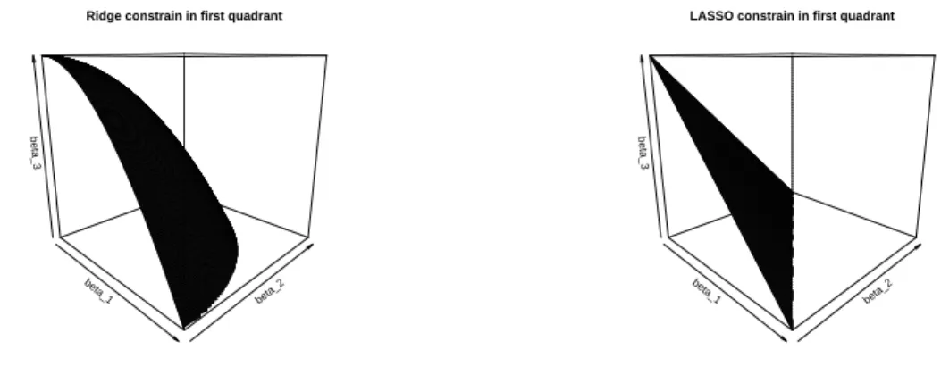
To visualize the constraint, we can plot a constraint for a β vector with 3 elements: β1, β2 and β3, this will result in format of 3-D graph. We plot the constraint of Ridge

(3.9) and LASSO (3.10) in first quadrant in figure 3.1. This is one-eighth of the space (all parameters are non-negative), and it can be extended to other seven quadrants and complete as a sphere for Ridge or an octahedron for LASSO. The estimation of β is constrained to be not beyond the surface. The loss function for Gaussian distribution is in a elliptical contour, for Poisson and Gamma it is a bit different, but still we can mimic the idea. Intuitively, the β contour is approaching from outside the space towards tangent to the surface, while minimizing the loss function. It will result in feasible possibility for LASSO surface to tangent the β contour on the edges, which means at least one of the βs is 0.

beta_1

beta_2 beta_3

Ridge constrain in first quadrant

beta_1

beta_2 beta_3

LASSO constrain in first quadrant

Figure 3.1: Ridge and LASSO constrain surface for 3 element β vector

3.1.2 Practice Procedure

Downsampling

In practice, we can not test all the data in relatively limited time, so what we did is downsample the data, particularly for frequency data. Keep in mind that our mission is not to estimate the rate by machine learning, but to discover the important variables to test in GLM, so as long as the relative ranking of variables is not mingled, we can refine

(21)

2.3, we have created a column of random integers range from 1 to 20, which partitions the dataset into 20 subsets, rows with random digit range from 1 to 16 are training and validation data, else are hold out data. Based on the law of large numbers, they should be roughly identically distributed with equal size. So when we take one of the subsets, it should contain most of the features of the entire dataset if the data size is huge enough. We keep all the observations with claim count greater than 0, because they reflect the information of levels in some variables indicate a high possibility of generating claim. For the ones without claim, we keep those observations with random integer column equals to 1, which takes roughly 5% of no claim observations. This method will result in enlarging the estimation of frequency, but by a roughly proportional way, so that the ranking of important variables is still stable.

Pre-selection of Variables

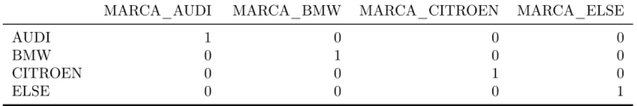
At the beginning of the project, we are not very familiar with all the variables, es-pecially those variables created very recently. As people have few experience with those variables, we keep those columns as they were, without grouping or converting them into ordinal numbers. In this case, the explanatory matrix we generate from the raw data will have too many columns if we include all variables. The method we use is one-hot encoding, also known as dummy variable transformation. For ex-ample in table 3.1 we are transforming the column MARCA (take 4 levels in variable VH010b_VIATURA_MARCA_ETxTIA_b as an example) into 4 dummy columns with boolean values 0 and 1. Notice that to be strict we should exclude 1 of these columns to avoid multicollinearity in the regression model, but in practice at least one of the variables will be set to zero, so it is OK to keep them like this.

Table 3.1: Dummy columns for categorical variable

MARCA_AUDI MARCA_BMW MARCA_CITROEN MARCA_ELSE

AUDI 1 0 0 0

BMW 0 1 0 0

CITROEN 0 0 1 0

ELSE 0 0 0 1

(22)

thou-Xu Zhifeng CHAPTER 3. DISCOVERING FEATURES AND INTERACTIONS

sands of columns thus almost impossible for the procedure to be processed without memory overflow. To solve this problem, we apply the pre-selection using XGBoost [Chen, He, Benesty, Khotilovich, Tang, Cho, Chen, Mitchell, Cano, Zhou, Li, Xie, Lin, Geng and Li, 2020] (will talk about this in section 3.2).

When we apply the XGBoost, we first tune the parameter using a grid, which collect all possible combinations of the different hyper parameters we chose in XGBoost. For ease of application, we select the combination of parameters which generates the smallest average cross validation error. Using the tuned parameter, we run XGBoost and get the initial ranking list of variables. As a rule of thumb, we take the top 100 variables appearing in the ranking list into the following procedure.

Ranking Variable Importance

Once the pre-selection is done, we take advantage of the shrinkage methods introduced in section 3.1.1. The response variables are the same as in GLM, for frequency model it is the frequency for the ith _{observation in (4.4) and for severity model it is the average}

size of claim in (4.10). For the weight we typically use the exposure for frequency model and count for severity model.

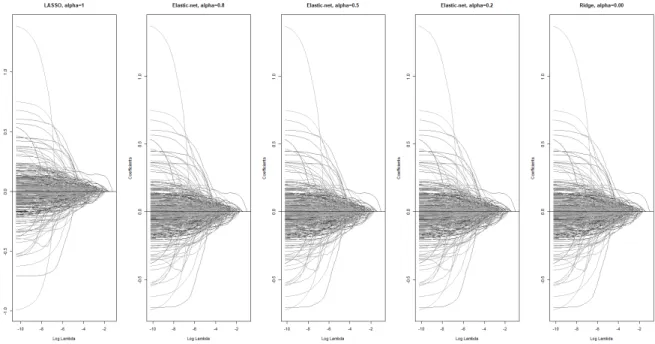
As can be seen in figure 3.2, the estimated βs shrinkage path is quiet similar among different values of α in (3.6), however, when we extract the estimation for βs, LASSO does really set some of the variables to exactly 0, while in Ridge there are a lot of small βs close to 0 but not equal to 0. So we decided to run the function based on pure LASSO, i.e., α = 1 to soft threshold the variables, keep less amount of variables to be fitted in our model.

(23)

Figure 3.2: Estimation of β shrinkage path among different α

We train our model on the different 5 training datasets, using the LASSO penalty. We choose the optimal λ in (3.5) by comparing the cross-validated average loss. Then the λ generating the lowest loss is selected as the optimal. In figure 3.3 we show the iteration of Gamma loss of our theft severity model for LASSO and Ridge. Although Ridge curves are more smoothly decreasing across iteration of λ, the Gamma loss in different partition of validation dataset come closer than Ridge when it is converging, it reassures the rationality of applying LASSO penalty.

−10 −8 −6 −4 −2 1000 2000 3000 4000 5000

FRB_S validation error iteration of LASSO

log(lambda) negativ e log lik elihood of Gamma validation_error_ 1 validation_error_ 2 validation_error_ 3 validation_error_ 4 validation_error_ 5 average validation error

−10 −8 −6 −4 −2 1000 2000 3000 4000 5000

FRB_S validation error iteration of Ridge

log(lambda) negativ e log lik elihood of Gamma validation_error_ 1 validation_error_ 2 validation_error_ 3 validation_error_ 4 validation_error_ 5 average validation error

Figure 3.3: Gamma loss on cross validation dataset for theft severity peril For each partitioned pair of training and validation set, we get the trained model and optimal λ. We predict response variable on validation dataset using fitted model

(24)

at tuning parameter equals the optimal λ. We average the estimated βs at optimal λ across all 5 folds to get the resulting βs more credible.

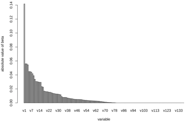
There are multiple ways to select the important features. The first method is to rank the importance of variables by their absolute values of βs. This method is used in R package caret [Kuhn, 2020], where the λ of the model is selected to be the one that generates the loss equals to the lowest possible loss plus 1 standard error of the minimum. This method is meaningful only when we standardized the data before executing the function, and the magnitude of β could be considered as an approximation of significance indices. If we sort and plot them in a bar chart, we can easily identify the βs which are significantly different from zero, and we simply keep the top variables in our GLM models. Or using a threshold value to filter the ones with βs greater than the threshold value. In figure 3.4 we plot the sorted average βs in our best model. The labels are replaced by “v1”, “v2”, etc. due to confidential reason. Note that we did not keep all the levels (almost 400 in total) so that the bars are not too thin to be visible.

v1 v7 v14 v22 v30 v38 v46 v54 v62 v70 v78 v86 v94 v103 v113 v123 v133

Average estimated beta by cross validation

variable absolute v alue of beta 0.00 0.02 0.04 0.06 0.08 0.10 0.12 0.14

Figure 3.4: Ranking of average estimated beta by cross validation of the theft severity model

(25)

we decrease the λ. This method is applicable for LASSO or elastic net with high propor-tion assign to LASSO component (α close to 1). This is similar to the idea of forward stepwise approach, but not exactly the same. When we set a huge λ, all the βs will be set to 0, so we have a model with β0 only, that is the mean model. By decreasing the

λ gradually, there will be 1 variable appearing, and that variable should be the most important variable. And then as we continue to decrease the λ, more variables will ap-pear, and we ensemble the model by adding those variables one by one to our model, until there are considerable amount of variables included. This method is more cautious compared with the previous one, as it choose the variables which add value to the model step by step, instead of a subset selected by one time.

In the last method, we first train our model using the same way above, then predict the model in validation set, compute the error by defined loss function, and set it as the referencing error. Further, we shuffle 1 column of the explanatory matrix in validation set at each time by resampling that column, and then predict the response variable on the validation set. We compute validation error, and compare it with the referencing error. If the error increase significantly, it means that the shuffled column reduced the predicting power significantly, so the variable is important. The difference can be ranked and standardized to represent the importance. Compared with the previous method, the advantage of this method is that it gives quantifiable importance of each variable. Interpreting Results

Applying the last method, we get the importance ranking result similar to what is shown in table 3.2.

Table 3.2: Feature importance ranking result.

Rank Variable Name Importance

1 VH0XX_4.abc 1.0000 2 SA1XX_c.xxx 0.7212 3 VH0XX_a.xx 0.3608 4 SA0XX_x 0.3391 5 GEOXX 0.3194 6 EXT0XX_e.xx 0.2707

(26)

Rank Variable Name Importance

7 VH0XX 0.2079

8 SA0XX 0.1879

9 VH0XX_xxx 0.1497

10 VH0XX_xxxxx 0.1487

... ... ...

In this table we have the variables ranked by their importance. As described above, the importance value is standardized by the error increment caused by shuffling that variable column, in proportion with the error increment of the top 1 ranked variable.

3.2 Interaction Detection

3.2.1 Extreme Gradient Boosting

When we have one variable related with another variable in a multivariate GLM in terms of coefficients, that means there are very likely to be interactions between these two vari-ables. It is not computationally easy to find the interactions exhaustively especially when we have huge number of variables.

We apply the extreme gradient boosting [Chen and Guestrin, 2016] method (marked as XGB), which is an implementation of gradient boosting [Friedman, 2000].

Loss Function and Approximation

The loss function to be minimized in extreme gradient boosting is LossXGB = n X i=1 l(yi, ˆyi) + K X k=1 Ω(fk) (3.11)

where l(yi, ˆyi) is the loss function of the ith prediction ˆyi, Ω(fk) is the penalty term for

(27)

Xu Zhifeng CHAPTER 3. DISCOVERING FEATURES AND INTERACTIONS Ω(fk) = γTk+ 1 2λ Tk X j=1 ωj2 (3.12)

including tuning parameters γ for Tk number of leaves in the kth tree and λ for sum of

squares of weights (denoted by ωj) of all Tk leaves.

By applying Taylor expansion to the tth _{iteration of the loss function, we get}

LossXGB(t) ≈ n X i=1 l(yi, ˆy (t−1) i + gift(xi) + 1 2hif 2 t(xi)) + Ω(ft) (3.13)

where gi and hi are gradient ∇ and Hessian ∇2 of the ith prediction’s loss function at

the (t − 1)th _{iteration. With this structure, the sequential tree can be built to find the}

minimization solution.

Sequential Tree Ensemble

XGB build trees starting from the simplest constant model, which is usually 0.5 by default, we mark it as T0, and calculate the loss based on T0 in (3.11), we mark it as

Residual0. Grow a tree on Residual0 to get the T1, ensemble T0 and T1 by the learning

rate η, we get the model M1 = T0 + ηT1, again we calculate the loss for M1, and grow

another tree T2 on Residual1, ensemble M2 = M1+ ηT2. Repeat this procedure round

after round, until the loss is almost not reducing during some pre-defined rounds. Interaction Detection

The interaction we are trying to detect is the so called “two-way interaction” which we will implement in our technical GLM model using Emblem software (see section 4.2.2). Interactions are ideally built on the residual of the main effects. Under this scope, the algorithm is: build a depth-1 ensemble tree with main effect captured first, and then build a depth-2 ensemble tree on the residual of the depth-1 tree. The variables used to split the branches in depth-2 tree model are collected as possible interaction pairs, ranked by gain quality in XGB.

However, this method is always generating few pairs of variables, due to the fact that when we are training the depth-1 model, the main effect is well captured by the model already, so the residual is not applicable to grow various different trees. As a result, we usually try another approach to detect the interactions, i.e., run the depth-2 tree model directly to generate more possible interacting results. The drawback is that we did not

(28)

take off the main effect from depth-1 model. But at the same time, the main effect in XGB depth-1 model is not the same as the linear predictor without interactions and polynomials in GLM model. So we are not losing a lot of robustness.

3.2.2 Practice Procedure

As described, we are trying to reduce the number of coefficients to be estimated in our GLM model without ignoring important features, i.e., we should take advantage of all the information we have. But there are some realistic restrictions and considerations that we will talk through in the following paragraphs.

Data Cleaning

In the original dataset, we have extreme case values for some of the variables, for example in the replicated theft frequency curve by variable driver age, as shown in figure 3.5:

Figure 3.5: Rescaled frequency average graph by variable driver age for theft peril

The yellow bars stand for exposure, and the values for observed and fitted averages are rescaled by dividing the value with the highest exposure (in this case age 44), the rescaled value close to 1 means it is close to the base. If we include observations in all range, the tree boosting procedure will be very likely to split the data at the “far left” or “far right” points on the horizontal axis, which is not a valuable information most of the time. Therefore, we pick the values that lies between feasible left and right points of the axis. (For instance in the driver’s age variable we pick those between 21 and 75.) This method also applies to the zero weighting of small exposure levels that can not

(29)

especially when they generate extreme rates.

Variable Converting

In the original data, there are different levels in each variable. Some of them are numeric, but most of them are bands or categorical strings. We need to transform the columns which has a numerical ordinal nature into numerical columns. For instance the band level 22.00-22.99 in some variable with ordinal nature, will be transformed to 22.5 in XGB explanatory matrix cell, which is the middle point of the band, so that the column will not be converted into dummy columns.

Parameter Tuning

The procedure of tuning parameter is subjective. Most of the time we have a grid of parameters to walk through, which is a matrix built up by combination of different parameters. After trying all the parameters in the grid, we can make our decision based on the lost behaviour in training set and/or validation set.

Here we use the example of the tuning parameters in the severity model of third party liability property damage peril. Figure 3.6 shows the validation error (negative log-likelihood of gamma distribution) iteration along number of rounds. Different curves have different parameters. Here we are tuning the parameter for η (stands for learning rate) and γ (stands for conservation of the model, which means minimum loss reduction to apply a new leaf note).

(30)

Xu Zhifeng CHAPTER 3. DISCOVERING FEATURES AND INTERACTIONS 0 20 40 60 80 8.095 8.097 8.099 8.101 RCM_S_validation_error_iteration number of iters v alid_gamma_nloglik eta= 0.4 gamma= 0 eta= 0.4 gamma= 4 eta= 0.4 gamma= 8 eta= 0.4 gamma= 12 eta= 0.3 gamma= 0 eta= 0.3 gamma= 4 eta= 0.3 gamma= 8 eta= 0.3 gamma= 12 eta= 0.2 gamma= 0 eta= 0.2 gamma= 4 eta= 0.2 gamma= 8 eta= 0.2 gamma= 12 eta= 0.1 gamma= 0 eta= 0.1 gamma= 4 eta= 0.1 gamma= 8 eta= 0.1 gamma= 12

Figure 3.6: Validation error iteration of different parameters of third party liability (property damage) severity model

In this figure we can observe that most of the parameter combinations have a rapid decrease along the first 20 rounds, and some of them turned to be flat afterwards while some of them fluctuate. We tend to choose number of rounds equals to the turning point, and the parameters that make the curve flat after the turning point. We choose η to be 0.2, γ to be 12 and number of rounds to be 20 in this example.

Ranking potential interactions

Applying the XGB procedure and using the tuned parameters, we can get the ranking presented in table 3.3, the “sImp” stands for split importance, and “intImp” stands for interaction importance.

Table 3.3: Potential interactions ranking result.

rank var1 split1 var2 split2 sImp intImp

1 DR0XX_XXX # VHXX_XX ## 1 1

2 SA0XX_XXX ##### TI0XX_XXX ##### 0.5693 0.6039

(31)

rank var1 split1 var2 split2 sImp intImp

3 DR0XX_XX ## VH0XX_XX ## 1 0.5673 4 GEO_XX #### VH0XX_XX ### 1 0.431 5 GEO_XX #### VH0XX_XX ### 1 0.3678 6 EXT0XX_XX # TI0XX_XX ### 0.6525 0.3615 6 EXT0XX_XX * TI0XX_XX *** 0.3475 0.3615 ... ... ... ... ... ... ...

In table 3.3 the results are ranked by the accumulating weighted gain on each pair of variables (var1 and var2), for instance the pair of variables SA0XX_XXX and TI0XX_XXX ranks number 2 in terms of the weighted gain. And inside this interaction, there are two different ways of splitting the variables: first way is to split SA0XX_XXX by #####, and split TI0XX_XXX by #####; second way is to split SA0XX_XXX by *****, and split TI0XX_XXX by *****. The relative importance score between these two splitting methods are 0.5693 and 0.4307, respectively, add up to 1.

Testing Interactions in GLM models

The result is ensemble tree built on XGB, it gives us the ranking of interactions based on the gains of each pair of variable combinations, it does not reflect the interaction under linear multiplication structure. To test the interactions performance in a GLM model, we first apply a GLM on these results. For instance, to pre-test the first inter-action’s significance in a GLM model, we run a GLM in R based on the combination of these variables: DR0XX_XXX*VHXX_XX, that is: DR0XX_XXX, VHXX_XX and DR0XX_XXX:VHXX_XX which stands for DR0XX_XXX multiplied by VHXX_XX. We need to take care of the magnitude of the product. If we multiply two variables with huge values, we could get convergence problem. So when we do the testing, normally we just test those pairs of variables with considerable values. The result will be like below:

(32)

Table 3.4: Pre-testing of interactions

variable name estimate SE z-value p-value

(Intercept) -84671.18 48537.14 -1.74 0.08 ... -14.86 10.08 -1.47 0.14 DR0XX_XXX 134.5 1654.51 0.08 0.94 VHXX_XX 15.15 32.79 0.46 0.64 DR0XX_XXX:VHXX_XX 2.81 0.57 4.91 0.00 ... ... ... ... ...

We can see that the p-value for the interaction term is quiet credible, regardless of the fact that the p-value for original variables are not so small which means this pair of variable is worth looking at in the full GLM model. This is a considerable finding because this indicates that the combined effect of these two variables are very significant and should be further analysed. The naive approach of testing this in the full GLM model is to split the variable by the split1 and split2 suggested by XGB. Which means we separate the data into two parts for each variable, resulting in only one extra term in the GLM, fit the splited factors and interactions in GLM model, looking at the betas and significance levels in both training and validation set. If they are both significant and in the same direction, then this pair of interaction is valid. In practice some of the interactions detected does not have a sensible meaning, then we may also not implement that although it is significant.

(33)

Chapter 4 Generalized Linear Models

Generalized linear models [Nelder and Wedderburn, 1972] (GLM) is a common insur-ance pricing predictive model. Although nowadays there are a lot of powerful machine learning tools to build regression models, the GLM still remains the key role in insurance pricing, due to the fact that GLM can efficiently establish tariff for regulatory purpose, and ease the communication between underwriting team and risk modelling team.

4.1 General Structure

The loss is separated by perils, for each peril we build different GLM models. Under each peril, our loss cost model is built on assumption that frequency is independent of severity, and claim count is Poisson distributed while severity is Gamma distributed, by assuming that they are independent, the aggregate loss can be modelled as a compound Poisson distribution.

The expected value of ith response variable is

µi = E(Yi) = g−1(ηi) (4.1)

where ηi is the linear predictor of ith response variable.

The variance of ith _{response variable in GLM is:}

V ar(Yi) =

φV (µi)

ωi

(34)

Xu Zhifeng CHAPTER 4. GENERALIZED LINEAR MODELS

where φ is the scale parameter and V (µi) is the variance function in terms of µi.

4.1.1 Frequency Model

For the frequency models we use Poisson regression, with logarithmic link-function. We assume that the number of claims occurring in the kth unit of exposure in the ith

obser-vation (denoted by Nik) is Poisson distributed with parameter fi, and the exposure of

ith observation is ωi. By definition of Poisson distribution, we have:

E(Nik) = V ar(Nik) = fi (4.3)

So the response variable Yi which represent the frequency of the ith observation is

calcu-lated by: Yi = Pωi k=1Nik ωi (4.4) By further assuming that each unit of exposure is independent [Anderson, Feldblum, Modlin, Schirmacher, Schirmacher and Thandi, 2007], we can get:

E(Yi) = Pωi k=1(E(Nik) ωi = ωifi ωi = fi (4.5) V ar(Yi) = 1 wi2 ωi X i=1 V ar(Nik) = 1 wi2 ωifi = fi ωi (4.6) so here the variance can be expressed as

V ar(Yi) =

µi

ωi (4.7)

V (µi) is just µi and scale parameter is 1. Note that in practice we have unfixed scale

parameter for quasi-Poisson [Wedderburn, 1974], i.e., a scale parameter not equals to 1, it is also called the overdispersion parameter, because the variance is higher than the variance in the original distribution.

4.1.2 Severity Model

(35)

so we choose logarithmic link-function to ease the expression of the model). We assume that the size of the kth_{claim in the i}th_{observation (denoted by X}

ik) is Gamma distributed

with parameter αi and θi, and the claim count of ith observation is ωi. By definition of

Gamma distribution, we have:

E(Xik) = αiθi (4.8)

V ar(Xik) = αiθi2 (4.9)

So the response variable Yiwhich represent the severity of the ithobservation is calculated

by: Yi = Pωi k=1Xik ωi (4.10) By further assuming that each claim is independent, we can get:

E(Yi) = Pωi k=1(E(Xik) ωi = ωiαiθi ωi = αiθi (4.11) V ar(Yi) = 1 wi2 ωi X i=1 V ar(Xik) = 1 wi2 ωiαiθi2 = αiθi2 ωi (4.12)

so here the variance can be expressed as V ar(Yi) = 1 αiµi 2 ωi (4.13) V (µi)is µ2i and scale parameter is

1 αi.

4.2 Complex Components

There are some components we need to add to explain the special characters that are not able to be captured in an ordinary GLM model. Including the orthogonal polynomials and interactions, etc.

4.2.1 Orthogonal Polynomials

Under linear predictor structure, for each explanatory variable (or each level of categori-cal variable), there is one beta assigned to it, and the component is linear as βixi for the

(36)

explana-Xu Zhifeng CHAPTER 4. GENERALIZED LINEAR MODELS

tory variable, there is a trend with curvature, then it is better to fit a polynomial. For a order q polynomial, the expression of the polynomial component will be Pq

m=1βiqxqi. It

is not linear in terms of explanatory variable xi, but it is linear in terms of βs, so we can

estimate it with the same algorithm for linear predictor. The new coefficients β∗_{s to be}

estimated in orthogonal polynomials are not coefficients for original variate powers xi,

x2_i, ... , xq_i, but the transformed variate powers P1(xi), P2(xi) , ... , Pq(xi) where Pt(xi)

itself is a tth _{order polynomial of x}

i, the q polynomials subject to constraint n

X

i=1

Pr(xi)Ps(xi) = 0, r 6= s, r, s ∈ 1, 2, ..., q (4.14)

The orthogonal polynomial predictor of variable xi to be estimated is

η(orth_poly)_x_i = αo+ α1P1(xi) + α2P2(xi) + ... + αqPq(xi) (4.15)

After applying orthogonal transformation, the different orders of components under the same variable are not correlated, and there will be no alias or generalized matrix inverse problems. However, the order of orthogonal polynomials should not be too high, to avoid overfitting and to ease the expression of the model.

4.2.2 Interactions

Interaction [Pedhazur and Schmelkin, 1991] in the linear model occurs when the effect on one variable is dependent on the level of another variable. [Anderson, Feldblum, Modlin, Schirmacher, Schirmacher and Thandi, 2007, pp. 59–77] interprets the interactions in GLM very well.

The simplest interaction is the two-way interaction, which involves two variables. Due to the nature of variable type, we have three scenarios:

1) Two categorical variables: variable 1 with k1 levels interact with variable 2 with k2

levels. For each variable there is 1 level assumed as base, the remaining levels can be packed with the non base levels in another variable. Result in adding (k1− 1)(k2 − 1)

factors in the original linear predictor (excluding those packed levels that does not have exposure), all the added factors are binary variables, with value taking either 0 or 1. 2) Two numerical (considered as continuous) variables, the interaction part is the product of them, that is adding one additional coefficient to be estimated. In figure 4.1, on the left hand-side panel is a flat plate stand for the linear predictor η = β + β x + β x ,

(37)

linear predictor plus an interaction term, i.e.,

η = β0 + β1x1+ β2x2+ β12x1x2 (4.16)

where β12 = 1for the middle and β12 = −1for the right. We can easily see that when we

have an interaction, the plate turns into a concave or convex surface. We can re-write the equation as

η = β0+ β1x1+ (β2+ β12x1)x2 (4.17)

The relative increase (or decrease) with respect to each unit of x2 is (β2 + β12x1). If

the sign of β12is the same as both β1 and β2, then velocity of increasing (or decreasing if

negative sign) is linearly increasing (or decreasing), like the graph in the middle. And if the sign of β12 is opposite to both β1 and β2, the interaction term will act like an offset

to the prediction. i.e., it will weaken the aggregate impact of increasing (or decreasing) in the original linear predictor.

x_1 x_2 y Linear predictor x_1 x_2 y Positive interaction x_1 x_2 y Negative interaction

Figure 4.1: Adding interaction effect to two continuous variables in the linear predictor

3) One numerical variable interact with another categorical variable with k levels, there will be (k − 1) new coefficients added in the model.

4.3 Model Selection Criteria

The criteria we use to select our model is not unilateral. Intuitively, the goal is to make the predicted curve fit the observed as good as possible without over or under estimation, at the same time avoid overfitting. To achieve this goal, we look at the graph as in figure 3.5, and analysis the statistics below.

(38)

4.3.1 Deviance and Chi-squared Test

When two models are nested (one model is a sub model of another), we usually test the models by investigating their deviance. The deviance is nothing but minus 2 times the log-likelihood. Assuming the two models are with p1 and p2 parameters respectively, the

model with p2 parameters is a sub model of the model with p1parameters. The difference

of two models’ deviance should asymptotically following a chi-square distribution with p1− p2 degrees of freedom, the test statistic is in equation (4.18).

∆Deviance = −2 n X i=1 loglik(yi, ηip2) − (−2 n X i=1 loglik(yi, ηip1)) a ∼ χ2_(p₁_−p₂₎ (4.18)

The chi-squared percentage (chi-squared p-value) is the probability of a random vari-able chi-squared distributed with p1 − p2 degrees of freedom to be greater than the

deviance difference of the two models. If the percentage is smaller than our significance threshold α, then the model with more parameters are significantly better than the model with less parameters.

4.3.2 Akaike Information Criterion

Akaike information criterion [Akaike, 1973], known as AIC, is a good tool to compare two models when they are not nested. AIC is simply the deviance plus 2 times numbers of parameters. AIC is a trade-off between deviance and model complexity. Normally we can compare two models by AIC values, and the smaller the better.

There are also some corrected versions of AIC, e.g. AICc [Sugiura, 1978]. AICc = AIC + 2p(p + 1) n − p − 1 = −2 n X i=1 loglik(yi, ηi) + 2p + 2p(p + 1) n − p − 1 (4.19)

If the number of observations is large enough, then the AICc should be similar to AIC.

4.4 Residual Analysis

The residual analysis is important for our model diagnosis and useful to detect departing such as under or over estimation.

(39)

There are multiple expressions of residual. The most common one is Pearson residual. ri_pearson=

yi − µi

pV (µi)

(4.20) In practice we use standardised Pearson residual most often, which is a modified version of Pearson residual.

r_{i_pearson}std = r√i_pearson 1 − hi

(4.21) where hi is the ith element in the diagonal of the hat matrix H. The hat matrix is as

below, where X is the design matrix and W is the weight diagonal matrix. H = W12X(XTW X)−1XTW

1

2 (4.22)

For a good model, the residuals should be centered around 0, and the ones with residuals higher than 0 should offset the ones with negative residuals in a balanced way. In the following figure, the axis “Transformed Fitted Value” is the linear predicted value, i.e., log(fitted value) under log-link structure, the axis “Standardized Pearson Residuals ” is the residual calculated by (4.21). The vertical axis is the frequency of it. We can see that the residual of third party liability property damage (marked as RCM) severity model is mostly distributed around 0, and the most popular fitted value is close to the log of mean, in this case around 7.1.

(40)

Chapter 5 Risk Technical Models

5.1 Initial Model Constructing

As discussed in the previous chapters, the risk technical models are built under GLM for main perils. We do forward stepwise regression for each model. As a team, we fo-cus on the same categories of variables mentioned in section 2.3 for different perils and testing the performance of our models in training and validation set, mainly focus on the consistency of the magnitude of estimated β, significance level or standard error percentage, and the relative impact of deviance (if only add component to the model) or AIC. We typically test the variables from the previous GLM models first, after adapting the previous model, we add new variables one by one, preferentially test the top ranked variables in our feature importance results (as in table 3.2).

After testing all the categories of variables, we begin to test interactions. The results from interactions detection (as in table 3.3) will be tested in the GLM models. The criteria of accepting the interaction is similar with the linear terms, i.e., β consistency, low standard error rate and significant reduction in deviance or AIC score.

5.2 Reviewing and Adjustments

The model is checked and reviewed in different phases of modelling. Since in practice, the data is modified or regrouped by demand of analyzing, there are some back and forth

(41)

Xu Zhifeng CHAPTER 5. RISK TECHNICAL MODELS

into the new data, and see if there is any level or variable missing. We also test the significance and consistency repeatedly.

We perform machine learning not only in the beginning of features and interactions selection. Because we changed our data structure, the variables and their levels are changing from the beginning of modelling, so we have to rerun the functions to get the most up-to-date results. Also, it is sometimes helpful to do the residual test, especially for the interaction detection. That is, take the residual of response variable after fitting a GLM using the fitted variables, and then run the depth-2 XGB tree function and get the potential interactions. But this requires a suitable transformation of residual, to be in cope with the distribution and link function structure. (For example non-negative response variable for log-link, natural number for Poisson distribution.)

The adjustment is applied when there are some validating new features to add in or non-validating old features to exclude from the model, either by newer result of machine learning or peer review.

5.3 Special Claims

5.3.1 Third Party Liability Personal Injury

If we split third party liability personal injury (marked as RCC) claims by a threshold of, for example, 500 thousand of euros, calculate the capped amount of RCC and excess amount exceeding 500 thousands, then we can find that more than 14% of the total amount of RCC claims comes from the excess claims, however the count of claims higher than 500 thousands is only about 0.2% of all claims. Meanwhile, about one-third of the claim counts are under a low threshold, let us say, 250 euros, which is a small size compared with average severity.

The original GLM model is built on all range of observed values. However, based on the special behavior described above, we focus our GLM on the claims higher than 250 euros and capped at 500 thousands euros, for the amount lower than 250 or excess of 500 thousands, we apply flat loading, and the probability of exceeding 250 euros is modelled by a logistic regression.

(42)

5.3.2 Windscreen

Although the assumed distribution is for the fixed explanatory variable rather than for the whole range of explanatory variable, it worth have a look at the whole data loss distribution. The severity of windscreen does not follow a Gamma distribution, as can be seen in the following figure, in the ECDF, there is clearly a jump around 250 euros, which means the severity has degenerate structure around some values. This is due to the distinction between windscreen repair claims and windscreen replacement claims.

Figure 5.1: Gamma fit test of windscreen severity

When we add a split point at 252, which is slightly higher than the jumping point in ECDF, and take the excess claims higher than 252, we can see there is no longer any degenerate value.

(43)

Figure 5.2: Gamma fit test of windscreen excess loss severity

The precise cut-off point for the degenerate value is hard to determine, and the probability of generating a large claim is not converging in the logistic regression model we fitted. When we dig deeper into the claims, we can see that the policies with repair shop agreements have much more stable severity compared with those policies without agreements. Almost all of the claims for policies with agreement are less than 255, while only around 40% of claims without agreement are less than 255. Therefore we split our severity data into two groups by having agreement or not, and model the severity without agreements by GLM, while using simplified model for the policies has agreements. By doing so, our estimation for the severity is more specific and accurate.

(44)

Chapter 6 Conclusions

6.1 Concluded Works

The preliminary risk technical models are successfully built for main perils, the variable categories are enriched, the accuracy of modelling dataset is improved.

The top ranked variables from penalized GLM play important roles in our GLM models, particularly, the ranking lists suggest the variables to look at in priority for the newly introduced variables. The XGB detected interactions also provide valuable information to bring in the model. All the perils have at least one interaction validating well in the models, but due to consideration of underwriting, we exclude some of them in the model. (e.g., one level in a variable is no longer going to be sold in the corresponding new tariff, so the interaction built based on the split by that level is excluded from the model.) When we combine the training and validation sets, adapt our model to the 80% data, more than 95% of the estimated coefficients are strongly significant, and are consistent with the training and validation estimation in sign.

6.2 Next Steps

Although the models are validating well in our preliminary testing, we need to test our models on the holdout dataset. The comparison between prediction and observed curves will give us more information about our models’ predictiveness, the closer the curves, the more confident we are with our model. The models will be refreshed if necessary.

(45)

Xu Zhifeng CHAPTER 6. CONCLUSIONS

The models will be imported into Earnix®1 _{and/or Radar}®2_{to perform rate aggregation}

and impact analysis.

After all, we will build restricted models by considering compliance, IT and economic issues. After the final testing and refreshment, we will deliver our model and present it to the stakeholder.

1_{https://earnix.com/}

(46)

Bibliography

Akaike, H. [1973], ‘Information theory and an extension of the maximum likelihood principle’, 2Nd International Symposium on Information Theory 73, 1033–1055. Anderson, D., Feldblum, S., Modlin, C., Schirmacher, D., Schirmacher, E. and Thandi,

N. [2007], A Practitioner’s Guide to Generalized Linear Models. URL: https://www.casact.org/pubs/dpp/dpp04/04dpp1.pdf

Chen, T. and Guestrin, C. [2016], ‘Xgboost’, Proceedings of the 22nd ACM SIGKDD International Conference on Knowledge Discovery and Data Mining .

URL: http://dx.doi.org/10.1145/2939672.2939785

Chen, T., He, T., Benesty, M., Khotilovich, V., Tang, Y., Cho, H., Chen, K., Mitchell, R., Cano, I., Zhou, T., Li, M., Xie, J., Lin, M., Geng, Y. and Li, Y. [2020], xgboost: Extreme Gradient Boosting. R package version 1.0.0.2.

URL: https://CRAN.R-project.org/package=xgboost

Friedman, J. [2000], ‘Greedy function approximation: A gradient boosting machine’, The Annals of Statistics 29.

Friedman, J., Hastie, T. and Tibshirani, R. [2010], ‘Regularization paths for generalized linear models via coordinate descent’, Journal of Statistical Software 33(1), 1–22. URL: http://www.jstatsoft.org/v33/i01/

Hastie, T., Tibshirani, R. and Friedman, J. [2001], The Elements of Statistical Learning, Springer Series in Statistics, Springer New York Inc., New York, NY, USA.

Hoerl, A. E. and Kennard, R. W. [1970], ‘Ridge regression: Biased estimation for nonorthogonal problems’, Technometrics 12(1), 55–67.

URL: https://www.tandfonline.com/doi/abs/10.1080/00401706.1970.10488634 Kuhn, M. [2020], caret: Classification and Regression Training. R package version 6.0-85.

(47)

Xu Zhifeng BIBLIOGRAPHY

LibertySeguros [2019a], ‘Liberty 2 rodas condições gerais e especiais’.

URL: https://www.libertyseguros.pt/Formulario/Documentacao/f63b170c-c2dd-4c6d-b34a-0e1a19ba9fe8

LibertySeguros [2019b], ‘Liberty sobre rodas condições gerais e especiais’.

URL: https://www.libertyseguros.pt/Formulario/Documentacao/c9d6141f-806d-4dc4-b6dc-01f169478635

Nelder, J. A. and Wedderburn, R. W. M. [1972], ‘Generalized linear models’, Journal of the Royal Statistical Society. Series A (General) 135(3), 370–384.

URL: http://www.jstor.org/stable/2344614

Pedhazur, E. and Schmelkin, L. [1991], Measurement, Design, and Analysis: An Inte-grated Approach, Lawrence Erlbaum Associates, Incorporated.

URL: https://books.google.es/books?id=K39lPwAACAAJ

Qian, W., Yang, Y. and Zou, H. [2013], HDtweedie: The Lasso for the Tweedie’s Com-pound Poisson Model Using an IRLS-BMD Algorithm. R package version 1.1.

URL: https://CRAN.R-project.org/package=HDtweedie

Riesz, F. [1910], ‘Untersuchungen über systeme integrierbarer funktionen’, Mathematis-che Annalen 69, 449–497.

URL: http://eudml.org/doc/158473

Simon, N., Friedman, J., Hastie, T. and Tibshirani, R. [2011], ‘Regularization paths for cox’s proportional hazards model via coordinate descent’, Journal of Statistical Software 39(5), 1–13.

URL: http://www.jstatsoft.org/v39/i05/

Stone, M. [1974], ‘Cross-validatory choice and assessment of statistical predictions’, Jour-nal of the Royal Statistical Society. Series B (Methodological) 36(2), 111–147.

Sugiura, N. [1978], ‘Further analysts of the data by akaike’ s information criterion and the finite corrections’, Communications in Statistics - Theory and Methods 7(1), 13– 26.

URL: https://doi.org/10.1080/03610927808827599

Tibshirani, R. [1996], ‘Regression shrinkage and selection via the lasso’, Journal of the Royal Statistical Society: Series B (Methodological) 58, 267–288.

(48)

Xu Zhifeng BIBLIOGRAPHY

Wedderburn, R. W. M. [1974], ‘Quasi-likelihood functions, generalized linear models, and the gauss-newton method’, Biometrika 61(3), 439–447.

Zou, H. and Hastie, T. [2005], ‘Regularization and variable selection via the elastic net (vol b 67, pg 301, 2005)’, Journal of the Royal Statistical Society Series B 67, 768–768.

Best practice of risk modelling in motor insurance : using GLM and Machine Learning approach

Master in

Actuarial Science

Master’s Final Work

Internship Report

Best Practice of Risk Modelling in Motor Insurance - Using GLM and

Machine Learning Approach

Xu Zhifeng

Faculty Advisor: João Manuel de Sousa Andrade e Silva

Industry Supervisor: Clayton Chiong

Acknowledgements

Abstract

Resumo

Contents

List of Figures

List of Tables

Chapter 1

Introduction

1.1

Motivation

1.2

Objectives

1.3

Structure

Chapter 2

Book Structure and Data

2.1

Coverage

2.1.1

Main Covers

2.1.2

Non-Main Covers

2.2

Bonus-Malus

2.3

Data and Software

Chapter 3

Discovering Features and Interactions

3.1

Variable Importance Ranking

3.1.1

Shrinkage Methods in Penalized GLM

3.1.2

Practice Procedure

3.2

Interaction Detection

3.2.1

Extreme Gradient Boosting

3.2.2

Practice Procedure

Chapter 4

Generalized Linear Models

4.1

General Structure

4.1.1

Frequency Model

4.1.2

Severity Model

4.2

Complex Components

4.2.1

Orthogonal Polynomials

4.2.2

Interactions

4.3

Model Selection Criteria

4.3.1

Deviance and Chi-squared Test

4.3.2

Akaike Information Criterion

4.4

Residual Analysis

Chapter 5

Risk Technical Models

5.1

Initial Model Constructing

5.2

Reviewing and Adjustments

5.3

Special Claims