DEPARTMENT OF CIVIL ENGINEERING
POSTGRADUATE PROGRAM IN CIVIL ENGINEERING
APPROACHES FOR AUTOMATED DAMAGE DETECTION IN
STRUCTURAL HEALTH MONITORING
RHARÃ DE ALMEIDA CARDOSO
DEPARTAMENTO DE ENGENHARIA CIVIL
PROGRAMA DE PÓS-GRADUAÇÃO EM ENGENHARIA CIVIL
TÉCNICAS PARA DETECÇÃO AUTOMÁTICA DE DANOS NO
MONITORAMENTO DA INTEGRIDADE ESTRUTURAL
RHARÃ DE ALMEIDA CARDOSO
APPROACHES FOR AUTOMATED DAMAGE DETECTION IN STRUCTURAL HEALTH MONITORING
Thesis presented to the Postgraduate Program in Civil Engineering, Department of Civil Engineering, Federal University of Ouro Preto, as partial fulfillment of the requirements for the degree of Doctor in Civil Engineering, area: Structures and construction.
Advisor: Alexandre Abrahão Cury Co-advisor: Flávio de Souza Barbosa
Ouro Preto
TÉCNICAS PARA DETECÇÃO AUTOMÁTICA DE DANOS NO MONITORAMENTO DA INTEGRIDADE ESTRUTURAL
Tese apresentada ao programa de Pós-Graduação do Departamento de Engenharia Civil da Escola de Minas da Universidade Federal de Ouro Preto, como parte dos requisitos mínimos para obtenção do título de Doutor em Engenharia Civil, área de concentração: Estruturas e construção.
Orientador: Alexandre Abrahão Cury Coorientador: Flávio de Souza Barbosa
Ouro Preto
Dedico meus sinceros e profundos agradecimentos ao professor Alexandre Cury, exemplo de bom mestre e amigo.
Também agradeço ao professor Flávio Barbosa pela parceria e pela abertura de oportunidades tão valiosas no âmbito acadêmico.
Com inteligência, empatia e cuidado, ambos contribuíram para tornar minha caminhada mais leve e virtuosa.
Por ter chegado até aqui, dou muitas graças por ter tido a oportunidade de passar por instituições de ensino públicas federais com tanta qualidade. De fato, o Brasil me proporcionou educação de alta qualidade e gratuita. Na minha trajetória acadêmica passei sete anos no Colégio Militar de Juiz de Fora, graduei-me em cinco anos na Universidade Federal de Juiz de Fora e realizei a pós-graduação por quase seis anos na Universidade Federal de Ouro Preto. No total, desfrutei de dezoito anos de trabalho nobre de homens e mulheres, funcionários públicos, que dão vida a estas belas instituições. Dou muitas graças a todos! Dou graças por ter a saudável companhia dos meus colegas de trabalho da PROINFRA da UFJF. Especialmente, agradeço aos pró-reitores: engenheira Janezete Marques e professor Marcos Tanure. Eles possibilitaram, de forma harmônica, um ambiente laboral no qual eu pude desenvolver minha tese em paralelo com as demais atividades de engenharia. Agradeço aos dois e também às chefias imediatas.
If you want to find the secrets of the Universe, think in terms of energy, frequency and vibration.
APPROACHES FOR AUTOMATED DAMAGE DETECTION IN STRUCTURAL HEALTH MONITORING
Rharã de Almeida Cardoso October/2018 Advisor: Alexandre Abrahão Cury
Co-advisor: Flávio de Souza Barbosa
Knowing the integrity of major structural systems in real-time and continuously during their operational service is a crucial requirement for manufacturers, owners, users and maintenance teams. This knowledge affords the stakeholders relevant structural performance information to drive design and production improvements, minimize maintenance costs, and increase the operational structure’s safety for the users. Among the several activities that comprise Structural Health Monitoring (SHM), damage detection is the core task to satisfy maintenance and safety aspects. Thus, an SHM program must be aided by computational tools capable of analyzing the acquired sensorial information continuously. Then, it must promptly yield one or more indicators of damage (or novelty) occurrence in the structure. Therefore, for a damage detection technique to be compatible with the scope of SHM, it should ideally respond automatically, in an unsupervised and continuous way, based solely on ambient vibration tests when the structure is under normal operation. Hence, this thesis presents two approaches: one based on the tracking of structural modal parameters, i.e., natural frequencies, damping ratios, and mode shapes; the other based on the analysis of raw acceleration measurements. The proposed methodologies were applied to real-case structures and showed promising performances when it comes to long-term, continuous and real-time monitoring.
TÉCNICAS PARA DETECÇÃO AUTOMÁTICA DE DANOS NO MONITORAMENTO DA INTEGRIDADE ESTRUTURAL
Rharã de Almeida Cardoso Outubro/2018 Orientador: Alexandre Abrahão Cury
Coorientador: Flávio de Souza Barbosa
Conhecer a integridade de sistemas estruturais de grande vulto durante o serviço, em tempo real e continuamente, é uma grande necessidade dos fabricantes, proprietários, concessionários, usuários finais e equipes de manutenção destes sistemas. Tal conhecimento provê aos gestores informações relevantes sobre o desempenho estrutural para direcionar melhorias no projeto e produção, além de minimizar custos de manutenção para o proprietário/concessionário e de aumentar a segurança de operação da estrutura para os usuários. Dentre as diversas atividades que compreendem o Monitoramento da Integridade Estrutural (MIE), a detecção de danos constitui o núcleo básico para atender aos aspectos de manutenção e segurança. Para tanto, o programa de MIE deve dispor de ferramentas computacionais capazes de analisar as informações adquiridas continuamente e em tempo real, fornecendo a cada momento um ou mais indicadores da ocorrência de dano (ou alteração) na estrutura. Portanto, para que uma técnica de detecção de danos seja compatível com o escopo do MIE ela deve, idealmente, prover respostas de forma automática, não supervisionada e contínua, baseando-se unicamente em testes de vibração ambiente com a estrutura em operação. Visando atingir estes objetivos, esta tese apresenta duas abordagens: uma baseada na evolução dos parâmetros modais, isto é, frequências naturais, taxas de amortecimento e modos de vibração; outra baseada na análise direta de medições de aceleração. As metodologias propostas foram avaliadas em estruturas reais e demonstraram desempenhos promissores quando aplicadas em monitoramentos de estruturas em longo prazo, contínuos e em tempo real.
This thesis is written as an effort to gather the last four years of research in a compact, yet comprehensible way: each chapter corresponds to a published/accepted or submitted paper. The methodologies proposed herein were assessed through numerical and experimental (laboratory and in situ) applications, as the techniques had their complexity increased and their accuracy improved.
The author would like to emphasize, however, that the present work is not only devoted to being a simple collection of papers. Instead, it was thought to create a smooth connection among the publications and to serve as a valuable manuscript on the subject for future reference.
Therefore, the text is structured in four parts as Fig. I shows.
Part I consists of a brief introduction, pointing out the relevance, motivation, and objectives of the developed research.
Part II and Part III constitute the core of this research. Within these parts, the reader will find one chapter for each one of the four written papers. The achieved advances and the connecting lines are reported through brief texts between the papers, at the beginning of each chapter.
Part IV concludes this thesis by highlighting the achieved milestones.
Fig. I Thesis’s outline.
MODAL IDENTIFICATION FOR DAMAGE DETECTION
PART II
RAW DATA PROCESSING FOR DAMAGE DETECTION
PART III
CHAPTER 2
Paper #1: A clustering-based strategy for automated structural modal identification
CHAPTER 3
Paper #2: A robust methodology for modal parameters estimation applied to SHM
CHAPTER 4
Paper #3: Unsupervised real-time SHM technique based on novelty indexes
CHAPTER 5
Paper #4: Automated real-time damage detection strategy using raw dynamic measurements
CONCLUSION
PART IV CHAPTER 6
PART I – INTRODUCTION ... 1
1 Introduction ... 2
1.1 Overview ... 2
1.2 Context ... 3
1.3 Damage and Novelty in SHM ... 4
1.4 Objectives ... 5
References ... 6
PART II – MODAL IDENTIFICATION FOR DAMAGE DETECTION ... 7
2 Paper #1 – A clustering-based strategy for automated structural modal identification .... 8
Abstract ... 9
2.1 Introduction and state of the art... 9
2.2 SSI-DATA ... 12
2.3 Automation methods for stabilization diagram interpretation ... 14
2.4 Results ... 19
2.5 Results discussion ... 32
2.6 Practical relevance and potential applications ... 34
Funding ... 34
References ... 35
3 Paper #2 – A robust methodology for modal parameters estimation applied to SHM ... 36
Abstract ... 37
3.1 Introduction ... 37
3.2 Data-driven Stochastic Subspace Identification ... 40
3.3 Automation methods for stabilization diagram interpretation ... 41
3.4 Results ... 49
PART III – RAW DATA PROCESSING FOR DAMAGE DETECTION ... 64
4 Paper #3 – Unsupervised real-time SHM technique based on novelty indexes ... 65
Abstract ... 66
4.1 Introduction ... 66
4.2 Feature Extraction and Data Fusion ... 69
4.3 Feature Classification ... 77
4.4 Experimental applications ... 79
4.5 Conclusion ... 86
Acknowledgements ... 86
References ... 87
5 Paper #4 – Automated real-time damage detection strategy using raw dynamic measurements ... 92
Abstract ... 93
5.1 Introduction ... 93
5.2 Feature Extraction and Data Fusion ... 96
5.3 Feature Classification ... 103
5.4 Application 1: Yellow Frame ... 107
5.5 Application 2: Concrete Bridge... 114
5.6 Conclusion ... 117
Acknowledgements ... 118
References ... 118
PART IV – CONCLUSION ... 122
PART I
INTRODUCTION
Chapter 1
Introduction
1 Introduction
1.1 Overview
Any mechanical structure is, ultimately, a dynamic system. Its vibrational behavior is continually informing about its state of integrity, or "health". This information can be acquired by various sensors measuring temperature, displacement, strain, acceleration, velocity, angular tilt, and so forth. Then, an appropriate software must process the acquired signals to allow the information to be accessible for human judgment. This is the core idea behind Structural Health Monitoring (SHM), as Fig. 1.1 summarizes.
Fig. 1.1 Extraction of intelligible information for structural health monitoring.
are supposed to perform the very task of detecting abnormalities in the system's behavior utilizing signal processing. Thus, it does not matter from which system this signal (response) is collected. Naturally, any application out of the civil engineering scope would possibly require some additional calibration.
1.2 Context
There has been an increasing awareness of the importance of damage prognosis programs in civil, mechanical and aerospace structures. A robust monitoring system could advise about the structure’s health state, informing about any incipient damage in real time and providing an estimate of the structure’s remaining useful life. The potential benefits that would result from such technology are enormous. The maintenance procedures for structures with such prognosis systems could change from being schedule-driven to condition-based. Hence, time, cost and labor requirements would be drastically saved, thus avoiding the interdiction of such structures. This would especially benefit aging structures, which are currently represented by the vast majority of viaducts, bridges, buildings, etc., in the world. Last, but not least, such a monitoring system would increase the structure’s safety for the users.
Thus, the acquisition of vibration tests and their subsequent analysis have gained great practical importance in the field of civil engineering. Studies have been published on the application of several types of instrumentation and data acquisition systems commonly used in the dynamic monitoring of large structures, such as the Rio-Niterói Bridge [1] in Brazil, the Z24 bridge [2] in Switzerland, and the Millau viaduct [3] in France.
Indeed, some strategic structures are monitored 24 hours a day, seven days a week – continuously or during time intervals – to provide data that can allow detecting structural problems in their initial stages, like cracks, excessive vibration, abnormal behaviors, etc. Additionally, such monitoring aims at providing a more in-depth assessment of structural reliability and vulnerability.
stays (from one tower) that initially went slack are the same in which a renowned structural engineer found possible damage during dynamic tests performed almost one year earlier. He warned the company that managed the bridge but said that they never followed up on his recommendation to conduct a thorough study and to instrument the bridge with permanent sensors. “Probably they underestimated the importance of the information,” said the engineer in an interview [4].
Fig. 1.2 Bridge collapses in Italy.
1.3 Damage and Novelty in SHM
To better understand the object of study of this work, it is imperative to distinguish the meaning of the terms structural damage and structural novelty.
therefore, does not imply that the structural system is damaged. For instance, a novelty can be caused by a structural reinforcement imposed by human intervention.
It is important to emphasize that the present work is devoted to providing tools for detecting structural novelty, which may or may not be characterized as damage. In practice, except for cases where there were structural reinforcements or intentional changes by human actions, almost every novelty is indeed damage. Therefore, the set of techniques developed within this thesis can provide useful tools to be placed into Level 1 of SHM Rytter’s classification:
Level 1: Is there any damage present in the structural system (detection)?
Level 2: Where is the damage located (location)?
Level 3: What is the damage magnitude (quantification)?
Level 4: What is the residual life of the structure (prognosis)?
1.4 Objectives
At first sight, an algorithm capable of detecting damage within an SHM context might be seen as a product of a simple strategy. However, the extensive literature review presented throughout the four papers showed that there are some challenges not yet transposed within this subject. In general, three obstacles pose an unpractical aspect to the existing detection algorithms (Level 1) for civil structures:
1. The lack of unsupervised techniques capable of detecting structural damage without relying on any prior knowledge about the structure’s condition;
2. The lack of strategies capable of robustly detecting structural damage automatically; 3. The lack of algorithms suitable for performing real-time detection.
Thus, the present work aims at presenting damage detection strategies that are unsupervised, automated and suitable for real-time SHM. These strategies are separated
References
[1] R.C. Batista and M.S. Pfeil. Reduction of vortex-induced oscillations of Rio-Niterói Bridge by dynamic control devices, Wind Engineering and Industrial Aerodynamics, 2000, 84(3), pp. 273-288.
[2] J. Maeck and G. De Roeck. Damage assessment using vibration analysis on the Z24-Bridge, Mechanical Systems and Signal Processing, 2003, 17(1), pp. 133-142.
[3] Y. Gautier, C. Cremona, O. Moretti. Experimental modal analysis of the Millau Bridge, Proceedings of the EVACES (Experimental Vibration Analysis for Civil Engineering Structures), 2005.
[4] J. Glanz et al. Genoa bridge collapse: the road to tragedy. New York Times, September 6, 2018.
PART II
MODAL IDENTIFICATION
FOR DAMAGE DETECTION
PART II
–
MODAL IDENTIFICATION FOR
Chapter 2
Paper #1 – A clustering
-
based strategy for
automated structural modal identification
2 Paper #1 – A clustering-based strategy for automated structural modal identification
One of the most common strategies to detect damage is based on the identification and tracking of structural modal parameters. Since the latter cannot exist without the former, the development and validation of tools for the automatic modal identification of structures under normal operation are the first main objective of this research. Therefore, this first research proposes a methodology for modal identification automatically, making it suitable for unsupervised real-time modal parameter based strategies for damage detection in SHM. In 2017, a paper was published in the journal “Structural Health Monitoring”.
Paper Information
Status Published in 2017
DOI https://doi.org/10.1177/1475921716689239
Publisher Structural Health Monitoring
ISSN 1475-9217; Qualis N/A; Impact Factor (2018): 3.798
Citation
Cardoso RA, Cury A, Barbosa F (2017). A clustering-based strategy for
Cardoso RA, Cury A, Barbosa F (2017). A clustering-based strategy for automated structural modal identification. Structural Health Monitoring, 17(2): 201-217.
Abstract
Structural health monitoring of civil infrastructures has great practical importance for engineers, owners and stakeholders. Numerous researches have been carried out using long-term monitoring, such as the Rio–Niterói Bridge in Brazil, the former Z24 Bridge in Switzerland and the Millau Bridge in France. In fact, some structures are continuously monitored to supply dynamic measurements that can be used for the identification of structural problems such as the presence of cracks, excessive vibration or even to perform a quite extensive structural evaluation concerning its reliability and life cycle. The outputs of such an analysis, commonly entitled modal identification, are the so-called modal parameters, that is, natural frequencies, damping rations and mode shapes. Therefore, the development and validation of tools for the automatic modal identification during normal operation is fundamental, as the success of subsequent damage detection algorithms depends on the accuracy of the modal parameters’ estimates. This work proposes a novel methodology to perform, automatically, the modal identification based on the modes’ estimates data generated by any parametric system identification method. To assess the proposed methodology, several tests are conducted using numerically generated signals, as well as experimental data obtained from a simply supported beam and from a motorway bridge.
2.1 Introduction and state of the art
First, for the sake of clarity, one should clearly distinguish modal parameter estimation (MPE) from modal tracking. The former consists of the estimation of modal parameters from a single record of measured data and the latter corresponds to tracking the evolution of the modal parameters of a structure through repeated MPE. This article focuses on the MPE process, which means that structural responses are evaluated independently. Therefore, what would naturally be the second step, related to modal tracking, will not be considered here.
Thus, concerning the parametric system identification techniques, one can enumerate the following two steps for the MPE:
1. Computation of the modes’ estimates for several orders of the parametric model, by fitting them to the response series;
2. Interpretation (in case of manual interpretation, the stabilization diagram would be one of the useful graphical tools used) of the modes’ estimates data by detecting spurious modes and selecting the physical ones.
In fact, without the automation of the MPE process, the user would be required to set several input parameters, making the modal identification procedure impractical to long-term applications such as the online health monitoring of structures. Therefore, especially over the last decade, several methods aiming at the reduction in the number of user-defined parameters are being developed [2–5], some of which reached the complete elimination of all manually specified parameters and, hence, are usually labelled as fully automated.
For instance, Reynders et al. [3] proposed a fully automated approach for the interpretation of a stabilization diagram. It was cleverly based on clustering techniques through three stages: a diagram pre-cleaning by means of a classification of all modes into two categories (possible physical or certainly spurious), a hierarchical clustering of the possible physical ones to group them together (automatic detection of vertical lines on diagram) and a final classification of the formed clusters into a physical or spurious condition. No user-defined parameter is needed whatsoever in the entire process.
focus on the elimination of all user-defined parameters (fully automation), but on the construction of a robust automated approach with some few easy configurable user settings, which are defined once, before starting the repetitive automated process itself. Thereby, this article presents an automated method for interpreting the stabilization diagram with just two easily user-defined parameters. Nowadays, the available time domain methods for operational modal analysis (OMA), explored in the work of Peeters and De Roeck [6], are essentially based on two types of models: discrete-time stochastic states-pace models and auto-regressive moving average (ARMA) or just auto-regressive (AR) models.
The formulations that use state-space models, designated stochastic subspace identification (SSI) methods, constitute the parametric approach that is more commonly adopted for civil engineering applications. The model can be identified either from correlations (or covariances) of the outputs: covariance-driven stochastic subspace identification (SSI-COV), or directly from time series collected at the tested structure by the use of projections [7]: data-driven stochastic subspace identification (SSI-DATA). As reported in the work of Peeters and De Roeck [6], these two methods are very closely related. Still, the SSI-COV has the advantage of being faster and based on simpler principles. The SSI-DATA, however, yields further outputs such as the decomposition of measured responses into modal contributions.
Considering the existence of a large number of alternative algorithms for OMA developed during the last decades, which sometimes are based on similar principles, this work focuses on the description of the SSI-DATA method. Since this method yields stabilization diagrams as outputs, the authors understand that these diagrams are a resourceful data for reliable structural modal identification. Moreover, when associated with clustering techniques, they are capable of providing very robust results. Thus, section 2.2 briefly discusses this method.
2.2 SSI-DATA
Since the work published in the 1990s [7], the application of SSI-DATA algorithms to determine the modal parameters of structures has been quite spread over the ambient vibration tests. State-space models are computed from output data (structure response) and can have their problem stated as following.
Given s measurements of the output yk ℝl generated by the unknown stochastic
system of order n
k+1 k k
k k k
A C
x x w
y x v (1) where xk ℝn is the state vector at a discrete-time instant k, wk and vk ℝn are zero mean,
white vector sequences with covariance matrix (at instants p and q with δ meaning the Kronecker delta)
T T
T
E p v 0
q q pq
p v
Q S S R w w vv , (2) determine the below:
The order n of the unknown system;
The system matrices Aℝn×nand Cℝl×n.
For this purpose, the SSI-DATA algorithm must consist of the following eight steps: 1. Organize the response series y (the only measured quantity) in a Hankel matrix Y
which can be partitioned into a past measurement’s matrix Yp and a future
measurement’s matrix Yf .
2. Calculate the orthogonal projection P of the row space of Yf on the row space of Yp
†T T
f p p p p
P Y Y Y Y
Y
(3) where •† denotes the Moore-Penrose pseudo-inverse of the matrix •.T 1 2
W PW USV (4) 4. Determine the system order n by inspecting the rank of S (the number of non-zero
singular values) and partition the SVD accordingly to obtain U1 and S1
1 TT 1
1 2 T
2
S 0 V USV U U
0 0 V (5)
5. Compute the extended observability matrix Γ 1 1/2 1 1 1
Γ W U S (6)
6. Determine, in a least square sense, the system (dynamic) matrix A from Γ as
†
A
Γ Γ
(7)where
Γ
denotes Γ without the last l (number of outputs) rows and Γdenotes Γ without the first l rows.7. Determine C as the first l rows of Γ.
8. Finally, knowing A and C, one can calculate the modal frequencies ωi, the modal
damping ratios ξi and the corresponding modal shapes i. This calculation is made
through the eigenvalue decomposition of matrix A as the following statements show
2100
i
i i i
i i i i i i i
(rad / s) f (Hz) ln Re (%) t
C
(8)
where μi is the ith discrete-time eigenvalue of A and i is its corresponding
These eight steps summarize the SSI-DATA routine which is, essentially, a fit of a state-space model to the temporal output data by means of the geometric projection of the row space of the future measurements onto the past measurements.
There are several valid sets of weighting matrices W1 and W2 to be used in equations (4) and (6). They determine the state-space basis in which the model will be identified. Special choices of these matrices correspond to algorithms described in the literature: principal component (PC), unweighted principal component (UPC) and canonical variate analysis (CVA). The PC algorithm is the one used in the applications shown in section ‘Results’.
It is necessary to point out that when one works with real structure response data, it is very hard to determine the system’s order through inspection of singular values like stated in the fourth step. This happens because the matrix S is actually full rank. Thus, a threshold would be necessary to consider a singular value as being null. Therefore, instead of creating ways for defining this threshold, the system order n is readily given as an input to the algorithm, which solves the problem, however, it creates the need for a further check whether this arbitrary order is able or not to accurately represent the actual data. One of the tools for this check is exactly the well-known stabilization diagram, where the modes’ estimates are plotted for various different system orders.
2.3 Automation methods for stabilization diagram
interpretation
As previously mentioned, the mode estimates (usually presented in a stabilization diagram) are supposed to be analysed to get physical modes apart from the spurious (numerical) ones. Spurious modes inevitably exist among the data, since they are a natural consequence of the parametric model’s attempt to better fit the response data.
measuring distances between modes’ estimates during the clustering process. Also, some additional modifications regarding filtering of spurious modes are included. Besides, a novel cluster regrouping technique is proposed.
For comparison purposes, section 2.3.1 presents a reference methodology, which corresponds to the basis of the algorithms proposed by Magalhães [2]. In section 2.3.2, the novel approach proposed by the authors is explained and all its contributions are highlighted. It is relevant to point out that both methods are suitable for the analysis of the outputs generated by any parametric identification technique that produces modes’ estimates (frequencies, damping ratios and modal shapes) for several model orders.
2.3.1 Reference methodology
In this approach, no pre-filter is applied to the modes’ estimates data, which means that the stabilization diagram would be still full of certainly spurious modes, that is, like those with extremely high or negative damping ratios. This method is based on a hierarchical clustering algorithm.
First, the dissimilarity (distance) measure between all pairs of estimated modes is calculated. The adopted ‘metric’ for calculation of such a distance is
1 MAC
i j
i, j i, j
j
f f d
f
(9)
where fi and fj are the natural frequencies of the modes’ estimates i and j, respectively. The
mode shape similarity between these two modes’ estimates is evaluated by the well-known modal assurance criterion (MAC). Moreover, one can note that for this metric, it is possible that di,j ≠ dj,i, which leads to an oddly asymmetric dissimilarity matrix.
Hierarchical clustering algorithms differ in the way they compute the distance between two already formed clusters. In this methodology, the single-linkage criterion is used, which means that the distance between two clusters will be considered as being equal to the smallest distance, also computed with equation (9), between objects inside these two clusters. This information allows constructing the hierarchical tree.
unknown quantity of clusters grouping spurious modes. Thus, the alternative strategy is the use of a distance limit (dlim). Such a distance is the criterion to prone the branches of the
hierarchical tree, generating clusters that are sufficiently distant from each other. Hence, the lower the limit, the higher the number of resulting clusters.
At this point, one has each cluster representing a single mode. To decide whether the mode is spurious or not, the clusters are ranked according to their number of elements. Thus, the top nm clusters with more elements are selected. Once physical modes are very consistent
for models with different orders, their clusters present a much higher number of elements than the clusters that contain numerical estimates (which present a higher scatter between models of different orders). Therefore, it is expected to find that the nm selected modes are indeed
physical. In practice, it is common to realize that the number of physical modes nm can be
guessed, for instance, by a simple preliminary frequency domain analysis.
Then, the damping ratios are taken into account by means of an outlier analysis within each selected cluster. This internal filtering eliminates the modes’ estimates with extreme damping ratio values, which are out of the range defined by ±2.698σ (standard deviation) that embraces 99.3% of the samples in a Gaussian distribution. Finally, each selected cluster produces average values of the modal parameters (natural frequency, modal damping ratio and mode shape), which are the outputs of the methodology.
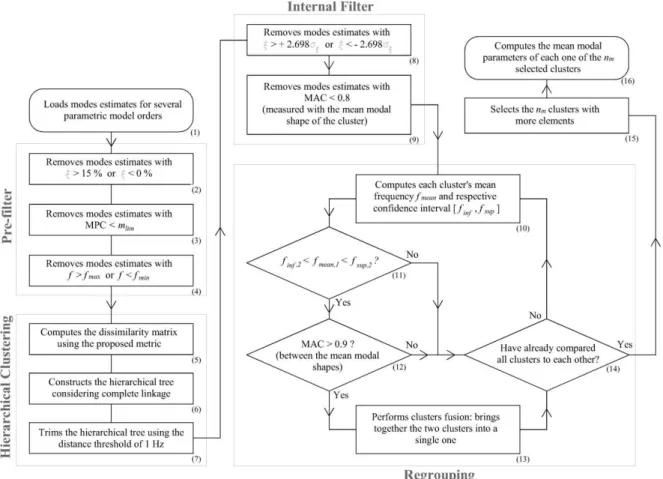
2.3.2 Proposed methodology
This method is also based on a hierarchical clustering algorithm. However, differently from the previous approach, one intends avoiding unnecessary computational efforts and aims to obtain better results from the clustering process. Thus, a pre-filter is applied on the modes’ estimates data, which removes all modes whose damping ratios are not between 0% and 15% (recommended for civil engineering structures). In addition, the stabilization diagram will have eliminated all modes with modal phase collinearity (MPC) indicator lower than a limit mlim in the [0, 1] interval of this criterion. The MPC index of a vector was stated by Juang
values closer to 0 show that the mode is either a spurious mode or the mode is significantly complex. Such an indicator is computed as
2MPC 1 2
1 2
(10)
where λ1 and λ2 are the eigenvalues of the matrix
xx xy xy yy S S S S
(11)
composed, as shown in equations (12), by the variances and covariance of the vectors r and i which are the real and imaginary parts of , respectively
T
xx r r
T
yy i i
T
xy r i
S S S (12)
Finally, the user may also have removed all modes’ estimates out of a range of frequencies specified (much like a ‘band-pass’ filter on the modes’ estimates data).
After having the modes’ estimates data processed by the pre-filter, a plot of the stabilization diagram would reveal that a significant amount of modes was removed, yielding a clearer aspect. Depending on the situation, and this is not rare, the removed modes may even represent more than 50% of the initial data. These removed modes’ estimates are considered as certainly spurious (or undesired) and will not be processed by the subsequent clustering algorithm.
To calculate the distance between the modes’ estimates i and j, a novel metric is used
1 MAC
i, j i j i, j
d f f c (13)
success of the method and, therefore, no deeper study about this topic was performed), which after some tests was stablished by the authors for being a satisfactory weight value. One should note that differently from equation (9), this metric leads to a perfectly symmetric dissimilarity matrix, that is, di,j=dj,i.
Then, the hierarchical clustering is applied. However, differently from the reference methodology, the distance between two already formed clusters is measured according to the complete linkage criterion, which means that such a distance is equivalent to the largest possible distance between two of their elements. Then, the hierarchical tree will be trimmed exactly like in the reference methodology by using a distance threshold dlim.
Differently from what the previous methodology does, the internal filter is here applied within the clusters before they are ranked according to their number of elements. This is done to penalize the clusters with high scatter (likely to be representing a numerical mode) before they could be ranked among the top nm modes that will be selected as physical.
Thereby, the internal filter removes outlier modes within the cluster considering not only damping ratios but also mode shapes. Mode estimates that have damping ratios out of the ±2.698σ range and/or have a lower than 0.8 MAC related to the cluster average mode shape are eliminated.
After this grouping process, depending on the dlim value, it is possible to find that
different clusters represent the very same physical mode. In other words, a single physical mode could have been split into two or more different clusters. Evidently, this phenomenon is to be avoided. Therefore, the authors propose a regrouping procedure to minimize this problem.
Finally, the top nm clusters (modes) with more elements are selected as being physical.
Then, each selected cluster has its average modal parameters (natural frequency, damping ratio and mode shape) calculated.
A flowchart of the developed methodology can be found in Fig. 2.1. The differences to the reference method, that is, the contribution of this work, is highlighted in red over the diagram shown in this figure.
The complete description and study of the proposed methodology can be found, in detail, in the work of Cardoso [12].
2.4 Results
2.4.1 Numerical experiment
Introduction
To initially evaluate the efficiency of the proposed method a numerical experiment was performed. The signals correspond to a hypothetical structure. Five degrees of freedom (DOFs) were considered.
Equation (14) describes a free damped vibration of a single-DOF dynamic system. In this equation, D represents the damped natural frequency that is approximately equal to, for
small damping rations ξ, the undamped natural frequency ω = 2πf. Besides, y(t) is the signal amplitude at a time instant t, ρ is an amplitude factor and θ is a phase constant.
2
1
( ) cos( ) i it
i Di i
i
y t
t
e
(14)The variables in the equation above were chosen in a manner that two modes with close natural frequencies were obtained. Table 2.1 shows the values of the dynamic parameters from this hypothetical system.
Table 2.1: Dynamic parameters of the hypothetical system.
f (Hz) ξ (%)
The modal shapes will not be analysed in this application. The objective here is to verify the capability of the proposed method for identifying correctly these closely spaced modes. First, a signal without noise will be processed. Then, 20% of white noise is artificially added. Such a noise was added to the signal according to equation (15). In this expression,
ynoise is the signal with noise, ymax is the maximum absolute value of y, β is a factor containing
the noise level (for instance, 0.2 = 20%) and χ is a random signal (white noise) generated by the computer, with amplitude varying from –1 to + 1.
max
( )
( )
. . ( )
noise
y
t
y t
y
t
(15) A 1000 Hz sampling rate was adopted, corresponding to 10 seconds of signal’s length. In this numerical experiment, the proposed methodology parameters were set equal to dlim = 1 Hz e nm = 2.Signal without noise
The pure signal (without noise), is shown in Fig. 2.2.
(a) (b)
Fig. 2.2 Time history of the generated signal (five channels) without noise: (a) complete signal and (b) zoom.
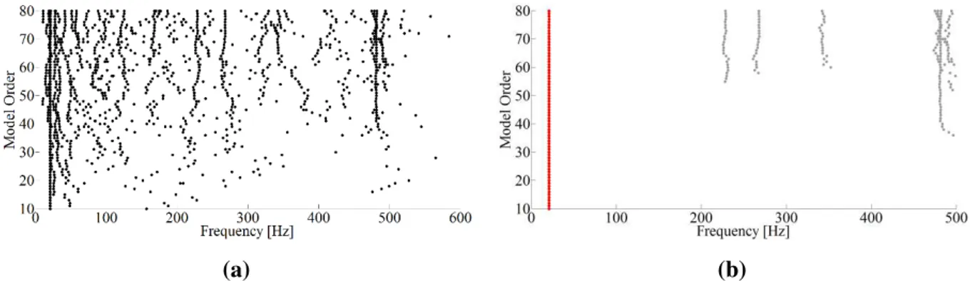
The SSI-DATA (PC) method was used to identify models with orders varying from 10 to 80. Once the dynamic system only has two physical modes, a large number of spurious modes appeared. This high-order modelling was intentional and aimed to turn the stabilization diagram more ‘polluted’, to test the capability of the developed method in distinguishing spurious modes from physical ones. In fact, in this study a model with order 4 would be enough to represent accurately the structural system.
modes were considered physical by the algorithm (top two clusters with more elements). Observing the processed diagram, one can say that, apparently, just one stable column was detected. However, when a zoom is given (Fig. 2.4), one can clearly see, the two closely spaced modes detected correctly.
(a) (b)
Fig. 2.3 Stabilization diagram: (a) before and (b) after the automated identification by the proposed method.
Fig. 2.4 Zoom of the stabilization diagram after algorithm’s application.
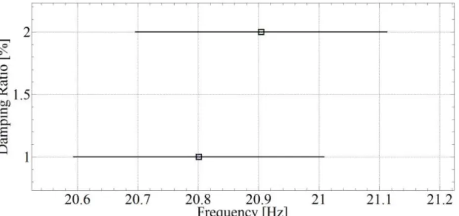
A frequency versus damping ratio plot of both identified modes can be found in Fig. 2.5. One can note, by such a figure, that there was no dispersion at all between the modes’ estimates within each one of the two clusters. Of course, this was already expected, once the signal is numerically generated and is free of noise.
Finally, Table 2.2 summarizes the results of the automated identification. It can be seen that the relative errors and the intra cluster standard deviations (σ) were technically null.
Signal with noise
equation (15), 20% (β = 0.2) of noise was added to the original signal. The high level of embedded noise, depicted in Fig. 2.6, can be seen.
Fig. 2.5 Frequency versus damping ratio plot of the two physical modes (clusters).
Table 2.2: Results of the automated modal identification.
f (Hz) σf (Hz) / error (%) ξ (%) σξ (%) / error (%)
Mode 1 20.79 0.003 / 0.05 0.96 0.00 / 4.00 Mode 2 20.94 0.017 / 0.19 2.06 0.01 / 2.91
Fig. 2.6 Complete time series of the five channels with a 20% noise.
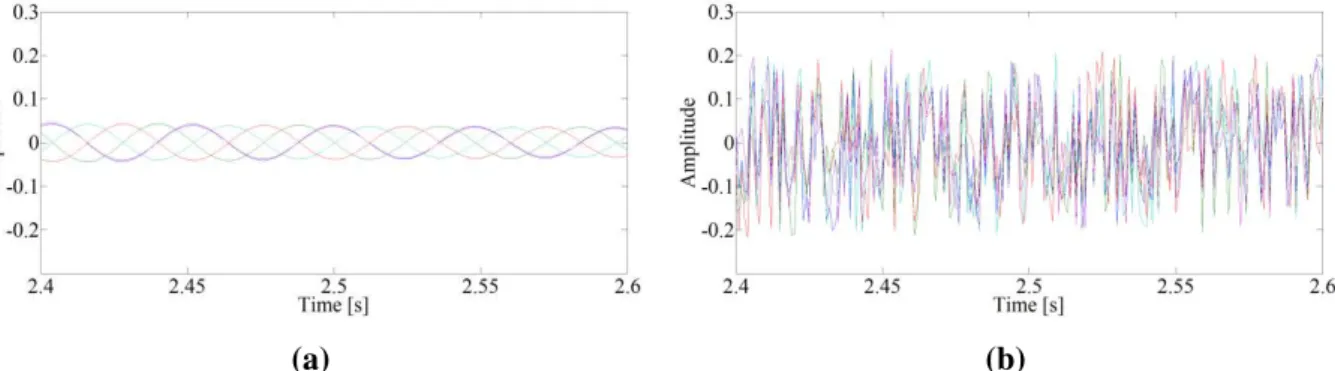
To allow a better insight about the effect of the noise level, Fig. 2.7 shows a part of the signal before and after the noise addition. It is clear that from a certain time instant, the amplitude of the noise is higher than the pure signal itself.
(a) (b)
Fig. 2.7 Part of the five channels’ signal: (a) before and (b) after noise addition.
(a) (b)
Fig. 2.8 Stabilization diagram generated by SSI-DATA (PC) algorithm: (a) complete diagram and (b) zoom.
After the application of the proposed algorithms, the stabilization diagram was the one shown in Fig. 2.9. One can note that the filters had less impact in this case: only 220 of the 1543 (14.3%) modes’ estimates were removed. Despite that, the red dots indicate that the developed method has identified, correctly, the physical modes.
(a) (b)
Fig. 2.9 Stabilization diagram after the proposed algorithm’s application: (a) complete diagram and (b) zoom.
significant amount of elements (corresponding to the two physical modes). This fact can be verified by means of Fig. 2.10. In such a figure, the red-headed stems represent the two selected clusters with more objects.
Fig. 2.10 Number of elements per cluster.
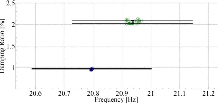
The frequency versus damping ratio plot of the selected modes estimates can be seen in Fig. 2.11. It is possible to note that a little dispersion in terms of frequency occurs within the cluster of higher frequency (green circles).
Fig. 2.11 Frequency versus damping ratio plot of the two physical modes (clusters).
Table 2.3: Results of the automated modal identification.
f (Hz) σf (Hz) / error (%) ξ (%) σξ (%) / error (%)
Mode 1 20.79 0.003 / 0.05 0.96 0.00 / 4.00 Mode 2 20.94 0.017 / 0.19 2.06 0.01 / 2.91
2.4.2 Laboratory experiment
This section presents the experimental tests conducted at COPPE/UFRJ laboratory on a simply supported steel beam depicted in Fig. 2.12. This beam is 1.46 m long with rectangular cross section (76.2 × 8.0 mm) and was instrumented with six piezoelectric accelerometers (PCB, 336C31). Data acquisition was carried out using Lynx ADS2002 equipment, which essentially is a conditioning/amplifier regulating system. This study considered random vibration tests (using a shaker). The random excitation was applied throughout the duration of the tests.
Fig. 2.12 Instrumented steel beam.
Again, the PC variant of SSI-DATA method was applied to the response series (six channels), leading to modes’ estimates of models with even orders from 10 to 120. Intending to create a basis for comparisons, the reference and the proposed methodologies are applied to the very same data set.
After a first quick manual judgement, the user-defined parameters were set up: dlim =
0.01 and nm = 8 (reference methodology); dlim = 1 Hz and nm = 5 (proposed methodology).
The mlim filter parameter was set to 0.9. Then, the different methodologies performed the
From Fig. 2.13, it is possible to see that the proposed filters had a great impact on the initial data set (Fig. 2.13b). Because of such a feature, 1015 (57.83%) of the 1755 modes’ estimates were readily removed. The stabilization diagrams depicted in this figure shows red dots for the automatically identified physical modes.
(a) (b)
Fig. 2.13 Stabilization diagrams after processing by (a) the reference methodology and (b) the proposed methodology.
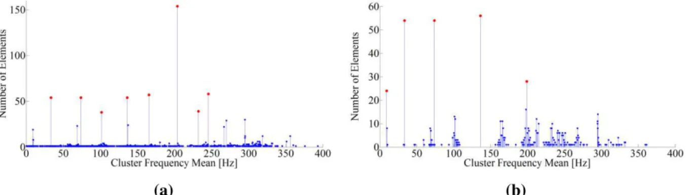
The number of elements within each formed cluster can be checked graphically in Fig. 2.14. Stems’ plot shown in Fig. 2.14a was generated by the reference methodology, while the stems’ plot shown in Fig. 2.14b was the result of the proposed methodology. The red head stems indicate the top nm clusters with more elements, which will be considered as being physical by the algorithms.
(a) (b)
Fig. 2.14 Number of elements grouped into each cluster by (a) the reference methodology and (b) the proposed methodology.
(red lines). The small font texts show the values (with standard deviations) of natural frequencies and damping ratios for each mode.
(a)
(b)
Fig. 2.15 Modal parameters obtained by (a) the reference method and (b) the proposed method.
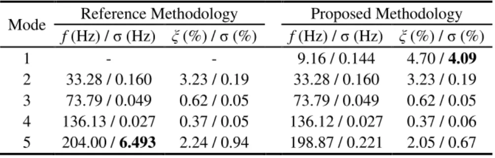
By analysing Table 2.4, one can conclude that the reference method not only ‘missed’ the first mode but also ‘captured’ the fifth mode with an unacceptable standard deviation (emphasized in bold) in terms of frequency. Differently, the proposed method identified the fifth mode with quite low standard deviation of frequencies. As can be seen, although the proposed method identified the first mode with high standard deviation of damping ratio (emphasized in bold), it was able to ‘capture’ the first mode of 9.16 Hz with just 0.14 Hz of standard deviation.
Table 2.4: Results of the automatic modal identification for the five vertical modes.
Mode Reference Methodology Proposed Methodology
f (Hz) / σ (Hz) ξ (%) / σ (%) f (Hz) / σ (Hz) ξ (%) / σ (%)
1 - - 9.16 / 0.144 4.70 / 4.09 2 33.28 / 0.160 3.23 / 0.19 33.28 / 0.160 3.23 / 0.19 3 73.79 / 0.049 0.62 / 0.05 73.79 / 0.049 0.62 / 0.05 4 136.13 / 0.027 0.37 / 0.05 136.12 / 0.027 0.37 / 0.06 5 204.00 / 6.493 2.24 / 0.94 198.87 / 0.221 2.05 / 0.67
2.4.3 PI-57 Oise Bridge
The PI-57 Bridge is a double-deck bridge located near the town of Senlis in France, crossing the Oise River and carrying the A1 motorway, which connects Paris to Lille (Fig. 2.16). The bridge, a 116.50-m-long, cast-in-place, post-tensioned segmental structure built in 1965, consists of three continuous spans of 18.00, 80.50 and 18.00 m. The two lateral spans play the role of counterweights.
Dynamic tests were performed under ambient excitation: the traffic was used as a source of excitation. Sixteen piezoelectric accelerometers (Bruel & Kjaer 4507B-005 with sensitivity of 1 V/g, frequency range from 0.4 to 6000 Hz, maximum operational level of 75 g, temperature range from –54 to +100 °C) have been installed on the bridge deck (Lille/Paris – Fig. 2.17). For the acceleration recording, a data programmable controller Gantner E-PAC DL was used and connected to an 8 GB USB flash drive. Data were transferred by a TCP/IP modem. Accelerations were filtered within the 0–30 Hz frequency range and sampling was set to 0.004 s (250 Hz) for 5 min. To make the data processing amenable, structural data were only recorded every 3 h over a 24-h time period and stored on a buffer hard disc.
Fig. 2.17 Plane view of the bridge with monitoring system.
Exactly like in the previous experiments, the SSI-DATA (PC) was applied to estimate structural modes considering both the reference methodology and the proposed methodology. However, differently from the previous test, in this application, the first method had dlim set to
0.1. On the other hand, the proposed algorithm had its distance threshold parameter set to the very same value of the last two experiments (dlim = 1 Hz), with one difference: here the
proposed method also eliminated (through its pre-filter) all the modes’ estimates with frequencies out of the 0–50 Hz range. Both methods had the parameter nm set to 8.
The stabilization diagrams after processing can be checked in Fig. 2.18. Again, as can be seen in the diagram generated by the proposed methodology (Fig. 2.18b), the filters had a significant impact on the initial data: 81.39% (1347) of the initial 1655 modes’ estimates were removed.
(a) (b)
Fig. 2.18 Stabilization diagrams after processing by (a) the reference methodology and (b) the proposed methodology.
(a) (b)
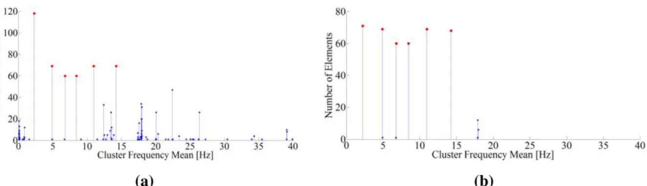
Fig. 2.19 Number of elements grouped into each cluster by (a) the reference methodology and (b) the proposed methodology.
Fig. 2.20 Mode shapes obtained by both methodologies.
nine vertical accelerometers in the plane view of Fig. 2.17, while the red corresponds to the lower line (in the plane view) of seven vertical accelerometers, as shown in the same figure.
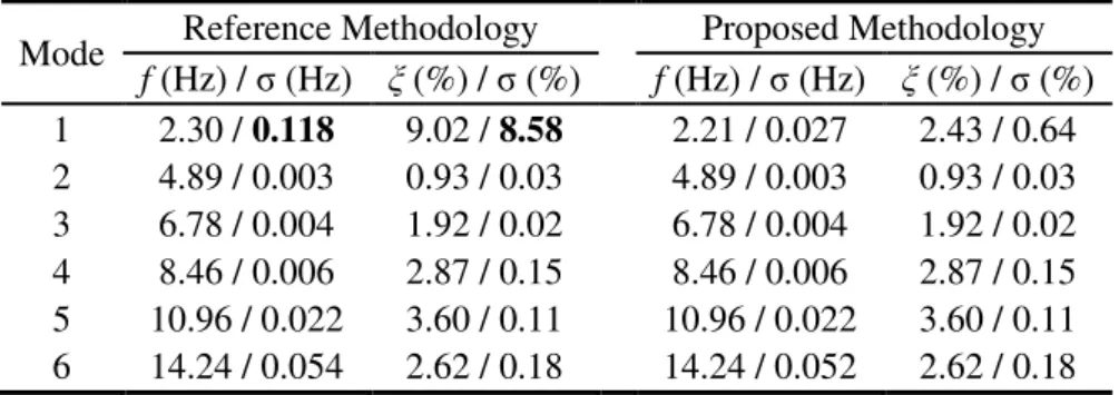
As shown in the results summarized in Table 2.5, for this application, the methodologies achieved very similar results, except for the higher standard deviation of the first mode identified by the reference methodology (emphasized in bold).
Table 2.5: Results of the automatic modal identification for both methodologies.
Mode Reference Methodology Proposed Methodology
f (Hz) / σ (Hz) ξ (%) / σ (%) f (Hz) / σ (Hz) ξ (%) / σ (%)
1 2.30 / 0.118 9.02 / 8.58 2.21 / 0.027 2.43 / 0.64 2 4.89 / 0.003 0.93 / 0.03 4.89 / 0.003 0.93 / 0.03 3 6.78 / 0.004 1.92 / 0.02 6.78 / 0.004 1.92 / 0.02 4 8.46 / 0.006 2.87 / 0.15 8.46 / 0.006 2.87 / 0.15 5 10.96 / 0.022 3.60 / 0.11 10.96 / 0.022 3.60 / 0.11 6 14.24 / 0.054 2.62 / 0.18 14.24 / 0.052 2.62 / 0.18
2.5 Results discussion
First, concerning the numerical experiment, one can conclude that the proposed method is suitable for identifying modes with very close natural frequencies, even in the presence of high levels of noise. However, it should be noted that the correct closely spaced modes’ identification is mainly due to the parametric modal identification method that was used (SSI-DATA).
The hierarchical clustering process over the modes’ estimates, or over the few remaining ones in case of the proposed method, deserves special attention. For the laboratory experiment, (Figs. 2.13 to 2.15), one may observe that the reference method was not able to identify the first vertical bending mode. However, in spite of the low-energy excitation of this mode during the tests, the proposed method did find this mode. Several values for the distance threshold (dlim) were tested the reference method to try to induce the algorithm to ‘catch’ the
first mode. However, the results were conclusive: as one increases the value of dlim, before the
low frequencies’ clusters could gain enough modes to be ranked among the top nm, the higher
frequencies’ clusters start to gather, in a too permissive way, a lot of modes (resulting in a fast growth of their stems –Fig. 2.14a). Consequently, a high scatter between modes belonging to a high-frequency cluster can be observed. Evidently, this excessive scattering is undesirable. A possible way of forcing the reference algorithm to catch the first mode is by keeping the dlim value fixed and increasing the nm parameter in an extreme conservative way. However,
one can say that this solution is not elegant, since a lot of spurious clusters (modes) would be selected along with the physical ones.
The high-frequency scattering phenomenon happens, mainly, for two reasons. First, the distance metric, which is written in equation (9), presents a dimensionless ratio of frequencies and, therefore, does not measure a distance between low-frequency modes with the same rigour as it measures a distance between high-frequency modes. Second, the single-linkage criterion for measuring the distance between two already formed clusters promotes a decrease in the heights of the hierarchical U-shaped branches, that is, it makes easier to ‘gather’ two clusters when compared to the complete linkage criterion.
On the other hand, the novel methodology proposed in this article is immune to such a phenomenon. That is due to the fact that the distance metric, stated in equation (13), does not contain any frequency ratio and, therefore, ensures that the distances between modes (with either high or low frequency) will be expressed by an absolute value in Hertz.
Another remarkable point is that the success of the algorithm proposed in this work is not as sensitive to the distance threshold as the reference algorithm is. For instance, in all tests, the user-defined limit for the proposed algorithm did not need to be adjusted (dlim = 1 Hz). This was achieved because of the novel metric and the proposed filters.
methodology, when compared to the reference in the studied applications, generated better results and, therefore, may represent an advance towards a more robust automatic modal identification method.
2.6 Practical relevance and potential applications
As the results show, the features included in the proposed methodology allowed accurate results for the automatic modal identification of civil engineering structures. With this algorithm, the large amount of data generated by the online dynamic monitoring can be treated automatically without significant loss of quality in the outputs. For the future, the suggested routine can be embedded in a standalone program with a graphical user interface to turn the application even more friendly and useful.
Although this article has used the SSI-DATA method to process the structure response, the proposed algorithm is also able to treat the outputs of any other parametric identification method that generates a stabilization diagram.
The proposed method is, therefore, a useful tool to modal identification of civil engineering structures subjected to ambient vibrations (OMA). Since this kind of test is by far the most practical one, it is of utmost importance that the algorithms dedicated to automatically interpret the data have a reliable efficiency, which was achieved in this work.
Funding
References
[1] Peeters B and De Roeck G. One year monitoring of the Z24-bridge: environmental effects versus damage effects. Earthq Eng Struct, 2001; 30: 149–171.
[2] Magalhães F. Operational modal analysis for testing and monitoring of bridges and special structures. PhD Thesis, University of Porto, Portugal, 2010.
[3] Reynders E, Houbrechts J and De Roeck G. Fully automated (operational) modal analysis. Mech Syst Signal Pr,2012; 29: 228–250.
[4] Ubertini F, Gentile C and Materazzi AL. Automated modal identification in operational conditions and its application to bridges. Eng Struct, 2013; 46: 264–278.
[5] Cabboi A. Automatic operational modal analysis: challenges and applications to historic structures and infrastructures. PhD Thesis, Università degli Studi di Cagliari, Italy,
2013.
[6] Peeters B and De Roeck G. Reference-based stochastic subspace identification for output-only modal analysis. Mech Syst Signal Pr 1999; 13(6): 855–878.
[7] Van Overschee P and De Moor B. Subspace identification for linear systems: theory, implementation and applications. Dordrecht: Kluwer Academic Publishers, 1996.
[8] Juang JN and Pappa RS. An eigensystem realization algorithm for modal parameter identification and model reduction. J Guid Control Dynam, 1985; 8(5): 620–627.
[9] Pappa RS, Elliott KB and Schenk A. Consistent-mode indicator for the eigensystem realization algorithm. J Guid Control Dynam, 1993; 16(5): 852–858.
[10] Vacher P, Jacqier B and Bucharles A. Extensions of the MAC criterion to complex modes. In: Proceedings of the international conference on noise and vibration engineering (ISMA 2010), Leuven, 20–22 September 2010.
[11] Yun GJ, Lee SG and Shang S. An improved mode accuracy indicator for eigensystem realization analysis (ERA) techniques. KSCE J Civ Eng,2012; 16(3): 377–387.
Chapter 3
Paper #2 – A robust methodology for modal
parameters estimation applied to SHM
3 Paper #2 – A robust methodology for modal parameters estimation applied to SHM
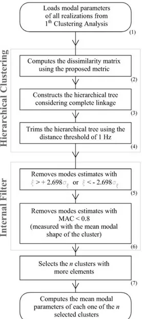
The previous chapter showed a method able to perform modal identification with little human judgment. Briefly, a stabilization diagram is interpreted by unsupervised machine learning algorithms. Although a high level of automation and accuracy has been achieved, the choice of the parametric model order and the choice of the number of desired modes consisted in a particular limitation for real-time SHM applications. Hence, complementary studies were carried out. This research culminated with the implementation of a new strategy: by automatically varying the model order and the number of desired modes, several stabilization diagrams are generated. Each one of them is interpreted by using the clustering procedures already presented. Afterward, the results of the various interpretations are subjected to another clustering step.
Consequently, despite the increase in computational effort, more automation and robustness were achieved. Thus, any abnormal deviations can be promptly detected, since natural frequencies, damping ratios and mode shape amplitudes are tracked over time. With this methodology, the objective related to the first approach of this thesis, i.e., to detect damage based on the tracking of structural modal parameters, is fulfilled. The resulting paper was published in the journal “Mechanical Systems and Signal Processing”.
Paper Information
Status Published in 2017
DOI https://doi.org/10.1016/j.ymssp.2017.03.021
Publisher Mechanical Systems and Signal Processing ISSN 0888-3270; Qualis A1; Impact Factor (2018): 4.370
Citation
Cardoso R, Cury A, Barbosa F (2017). A robust methodology for modal parameters estimation applied to SHM. Mechanical Systems and Signal Processing, 95(2017): 24-41.
Abstract
The subject of structural health monitoring is drawing more and more attention over the last years. Many vibration-based techniques aiming at detecting small structural changes or even damage have been developed or enhanced through successive researches. Lately, several studies have focused on the use of raw dynamic data to assess information about structural condition. Despite this trend and much skepticism, many methods still rely on the use of modal parameters as fundamental data for damage detection. Therefore, it is of utmost importance that modal identification procedures are performed with a sufficient level of precision and automation. To fulfill these requirements, this paper presents a novel automated time-domain methodology to identify modal parameters based on a two-step clustering analysis. The first step consists in clustering modes estimates from parametric models of different orders, usually presented in stabilization diagrams. In an automated manner, the first clustering analysis indicates which estimates correspond to physical modes. To circumvent the detection of spurious modes or the loss of physical ones, a second clustering step is then performed. The second step consists in the data mining of information gathered from the first step. To attest the robustness and efficiency of the proposed methodology, numerically generated signals as well as experimental data obtained from a simply supported beam tested in laboratory and from a railway bridge are utilized. The results appeared to be more robust and accurate comparing to those obtained from methods based on one-step clustering analysis.
3.1 Introduction
relationship that exists between modal parameters and structural stiffness and mass explains this tendency. Therefore, it is not by chance that modal parameters are widely used in continuous dynamic monitoring systems of important civil structures, such as long-span bridges, stadiums, tall buildings, among others [3,4].
Continuous monitoring systems are especially relevant due to their preventive nature, since they can be inserted in maintenance programs and actually support detecting unusual structural behaviors. Abnormal structural states are often assessed by observing the variation of modal parameters over time. Hence, the modal identification procedure becomes of utmost importance and deserves special attention concerning its accuracy, robustness and automation to make it viable in a context of online monitoring. Due to the necessity of an automatic feature, parametric time-domain based identification methods have been preferred among engineers. Mostly, the so-called SSI (Stochastic Subspace Identification) methods, which use discrete-time stochastic state-space models, are very suitable in this case due to their capacity to identify closely-spaced frequencies. Moreover, they provide useful ready-to-use data for feature extraction by means of clustering techniques or any other data mining methods.
At this point, it is worth highlighting the difference between modal parameter estimation (MPE) and modal tracking (MT). The former consists in the estimation of modal parameters from a single record of measured data and the latter corresponds to tracking the evolution of modal parameters of a structure through repeated MPE. This paper is limited to MPE, not involving what would be a complementary task to online monitoring (MT). Therefore, isolated signals of a given dynamic test in a structure are evaluated independently, with no time tracking of modal parameters.
In fact, without the automation of the MPE process, a lot of user interaction over a large amount of measured vibration data would be required, leading to an impossibility of practical applications such as the health monitoring of important infrastructures. Therefore, especially over the last decade, several methods aiming the reduction of the number of user-defined parameters have been developed [5–8], some of which reached the complete elimination of all manually specified parameters and, thus, are usually labelled as fully automated.
classification of all modes into two categories (possibly physical or certainly spurious); a hierarchical clustering of the possible physical ones to group them together; and a final classification of the formed clusters into a physical or spurious condition. No user-defined parameter is needed in the entire process.
However, despite the observed advances, practice has been showing that even the most sophisticated automated process of MPE has to be preliminarily checked or tuned in order to fit a unique behavior of the analyzed structure. Otherwise, the method might become too much vulnerable to fail due to different identification scenarios, like different levels of frequencies and damping ratios, different complexities of modal shapes, several types of external excitation sources and different amounts of signal noise. For that reason, the present work focus on the development of a robust automated approach that depends on just few easy-to-set user-defined parameters.
Currently, the available time domain methods for operational modal analysis (OMA), explored in the work of Peeters and De Roeck [9], are essentially based on two types of models: discrete-time stochastic state space models and ARMA (Auto- Regressive Moving Average) or just AR (Auto-Regressive) models. The models can be identified either from correlations (or covariances) of the outputs: Covariance driven Stochastic Subspace Identification – SSI COV; or directly from time series collected at the tested structure by the use of projections [10]: Data driven Stochastic Subspace Identification – SSI-DATA. As reported in the work of [9], these two methods are very closely related. Still, the SSI-COV has the advantage of being faster and based on simpler principles, whereas the SSI-DATA allows obtaining some further information with a convenient post-processing, as for instance, the decomposition of the measured response into modal contributions.
This work focuses on the use of the SSI-DATA method, since this method yields stabilization diagrams as outputs, which are a resourceful data for reliable structural modal identification. Moreover, when associated with clustering techniques, they are capable of providing very robust results. Thus, Section 3.2 briefly discusses the SSI DATA method (a more thorough description can be found in reference [10]).