MASTER IN FINANCE
MASTER’S FINAL WORK
PROJECT
VOLATILITY ADJUSTED MOMENTUM STRATEGY:
IMPLEMENTATION AND PERFORMANCE
EVALUATION
FILIPE JO ˜
AO DA ASSUNC
¸ ˜
AO JANEIRO
MASTER IN FINANCE
MASTER’S FINAL WORK
PROJECT
VOLATILITY ADJUSTED MOMENTUM STRATEGY:
IMPLEMENTATION AND PERFORMANCE
EVALUATION
FILIPE JO ˜
AO DA ASSUNC
¸ ˜
AO JANEIRO
SUPERVISOR:
RAQUEL M. GASPAR
Abstract
We implement and detail a stock trading strategy, named volatility adjusted
mo-mentum strategy (VAMS) that minimizes the negative impact human emotions can
instill in traders investment decisions. It withdraws the randomness and subjective
interpretation from the portfolio asset selection. Our fully automatized approach
takes advantage of a pervasive and well documented financial inefficiency, the
so-called: momentum effect. By adjusting momentum to volatility and using risk parity in asset portfolio weighting, our findings support that in the long run, investors can
actively expect to outperform the S&P500 benchmark. This strategy has the
po-tential of exhibiting higher returns with lower exposure to risk, and presents the
capability to diminish greatly the impact of bear markets in portfolio management.
Key words
Momentum, human emotions, risk management, adjusted volatility, risk parity,
port-folio management.
Resumo
Implementamos e detalhamos uma estrat´egia de negocia¸c˜ao em a¸c˜oes, de nome
es-trat´egia de momentum com volatilidade ajustada, que minimiza o impacto negativo
que as emo¸c˜oes humanas podem incutir aos traders nas suas decis˜oes de
investi-mento. Remove a aleatoriedade e interpreta¸c˜ao subjetiva na sele¸c˜ao dos ativos
con-stituintes do portf´olio. A nossa abordagem totalmente automatizada tira proveito
de uma generalizada e bem documentada ineficiˆencia financeira, o efeito momen-tum. Ao ajustar o momentum `a volatilidade e usando paridade de risco no peso a atribuir aos activos no portf´olio, os nossos resultados suportam que a longo prazo,
os investidores podem ativamente esperar obter melhor performance que o mercado
de referˆencia S&P500. Esta estrat´egia tem o potencial de exibir maiores retornos
com menor exposi¸c˜ao ao risco, e apresenta a capacidade de diminuir
consideravel-mente as grandes viragens para terreno negativo do mercado bolsista, na gest˜ao de
portf´olios.
Palavras chave
Momentum, emo¸c˜oes humanas, gest˜ao de risco, volatilidade ajustada, paridade de
Acknowledgements
I dedicate this work to my parents, Maria Celeste Janeiro and Jo˜ao Herm´ınio Janeiro.
Without their example, guidance, help and unlimited support I would have never
been able to succeed in my studies, both in engineering and finance.
First and foremost, I would like to express my gratitude to my supervisor, Professor
Raquel M. Gaspar, for her guidance, patience, and providing my research with great
corrections and suggestions.
I also would like to thank Professor Clara Raposo, for her excellent advice during
my Masters in Finance. I am very grateful for the given opportunity of belonging
to the first CFA Challenge ISEG team ever.
To my dear friend and CFA team college, Professor Victor Barros, thank you for
your constant support and superior suggestions. You are the perfect definition of
perseverance and an example to everyone.
The greatest thanks I leave to my friends, who over the years continue to put up
with the complexity of my being.
Finally, I want to make the most sincere gratitude to all those who throughout my
life, helped and supported me, but unfortunately as consequence of life vicissitudes
are no longer part of it.
Risk comes from not knowing what you are doing.
Contents
Contents iv
Acronyms v
List of Figures v
List of Tables vi
1 Introduction 1
2 Literature Review 4
2.1 Investors performance and behavior . . . 4
2.2 Momentum - The Premier Market Anomaly . . . 8
2.3 The Risk Parity Weighting Process . . . 10
3 The trading strategy 12 3.1 The strategy rules . . . 12
3.2 Volatility adjusted momentum process . . . 18
3.3 Risk parity positions and rebalancing process . . . 21
3.3.1 Position size . . . 21
3.3.2 Position rebalancing . . . 22
4 Data and methodology 23 4.1 Data . . . 23
4.2 Methodology . . . 24
5 Results 26 5.1 VAMS vs benchmark performance . . . 26
5.2 VAMS trading costs stress test . . . 33
5.3 VAMS out-of-sample process . . . 34
6 Conclusion 35
Bibliography 36
Acronyms
ATR average true range. 21, 22
EMH efficient market hypothesis. 4, 8, 9
SMA(100) 100 days simple moving average. 13–16
SMA(200) 200 days simple moving average. 13, 16
SMA(50) 50 days simple moving average. 13
SMMA smoothed moving average. 21
VAMS volatility adjusted momentum strategy. ii, v, vi, 1–3, 12–15, 18, 23–29, 31, 33–35
VaR value-at-risk. 26–28, 34, 35
List of Figures
1 Trading rules loop chart . . . 17 2 Volatility adjusted momentum examples . . . 20
3 VAMS implementation flowchart . . . 25
4 Absolute returns dynamic performance - Jan 2005 to Dec 2015 . . . 27 5 Annualized returns dynamic performance - Jan 2005 to Dec 2015 . . 28 6 VAMS vs S&P500 weekly returns histograms - Multiperiods . . . . 30 7 Trading costs stress test - Jan 2005 to Dec 2015 . . . 33 8 Absolute returns and index SMA200 evolution - Jan 16 to Jul 16 . . 34
List of Tables
I Ranked constituents S&P500 at 07/01/2015 . . . 15
II 11 years VAMS performance (Jan 2005 - Dec 2015) . . . 27
III Risk indicators evolution by year - Jan 2005 to Dec 2015 . . . 29
IV VAMS and S&P500 descriptive statistics . . . 30
V Strategy and benchmark main results . . . 32
VI 2016 Out-of-sample VAMS vs S&P500 performance . . . 34
VII 2016 Out-of-sample descriptive statistics . . . 34
VIII Yearly relative returns - 2005 to 2015 . . . 40
IX VAMS vs S&P500 constituents, 11 years investment (2005-2015) . . 40
X Risk indicators evolution by year - Jan 2006 to Dec 2015 . . . 42
XI Risk indicators evolution by year - Jan 2007 to Dec 2015 . . . 42
XII Risk indicators evolution by year - Jan 2008 to Dec 2015 . . . 42
XIII Risk indicators evolution by year - Jan 2009 to Dec 2015 . . . 42
XIV Risk indicators evolution by year - Jan 2010 to Dec 2015 . . . 43
XV Risk indicators evolution by year - Jan 2011 to Dec 2015 . . . 43
XVI Risk indicators evolution by year - Jan 2012 to Dec 2015 . . . 43
XVII Risk indicators evolution by year - Jan 2013 to Dec 2015 . . . 43
XVIII Risk indicators evolution by year - Jan 2014 to Dec 2015 . . . 43
Chapter 1
Introduction
A significant amount of people around the world invest in some kind of financial
asset. Stock ownership is definitely among one of the most preferable choices. As
noticed by Gallup polls1, in 2015 more than half of all Americans owned stocks in
their personal portfolio, having this amount achieved a 65% score in 2007. Given
this information, a question immediately pops-up: how well is expected an average
individual investor to perform?
In a world continuously more complex, competitive and demanding, finding
evi-dences that investors can beat the market may not be very promising. Barber and
Odean (2011) provide powerful insights about how in theory, investors hold well
diversified portfolios and trade infrequently, looking to minimizing all type of costs,
but in practice, they behave rather differently. The authors document individuals
performance being poor, underperforming standard benchmarks, and usually selling
winning investments while holding losing investments, the disposition effect, firstly documented by Shefrin and Statman (1985)2. Human emotions seem to play a
mas-sive role in investment decisions, largely contributing towards a poor performance.
Overconfidence, limited attention, seeking pleasure, failure to diversify are also other
behaviors displayed by individual investors while investing.
This project aims at increasing the individual investors’ chances of succeed in stock
investments. In order to accomplish this milestone, we will detail and implement an
automatized trading strategy (VAMS) that overcomes the human emotion factor in
the decision investing process. As individuals have a limited amount of attention
they can assign to the investment process, we present a systematic approach based
1
http://www.gallup.com
2
on a exact set of rules. This way investors can head their attention, eliminating
overreactions that would occur from noise and irrelevant information.
The strategy under analysis has been proposed by Clenow (2015), having in mind the
discovery of Jegadeesh and Titman (1993). One of the strongest and most pervasive
financial phenomena: the momentum effect. As acknowledge by Fama and French (2008) momentum is the premier market anomaly. Their research observes that the abnormal returns associated with momentum are pervasive, and we want to
capitalize it too.
Momentum investing is about buying stocks that are moving up. When price is
increasing, we buy with the expectation that the price continues to increase. We
should remember that it is impossible to dissociate returns from risk. Risk is one of
the most important features to be taken in consideration when investing. Therefore,
we seek to minimize risk by adjusting momentum to volatility and by using risk
parity3 in asset portfolio weighting.
The main contribution of this work to the literature is reinforcing the potential of
au-tomatized quantitative momentum investment strategies4, providing the obliteration
of human emotions in investment decisions, and consequently enabling the
expec-tation of possible enduring higher performance. Specially the capability of stanch
bear markets negative impacts. Passive investment strategies have gather many
supporters in the last years5, but are unable to present such capability6. VAMS has
the potential of achieving higher returns when compared to passively investing in
the S&P500 benchmark, while minimizing risk and drawdowns7.
Our study also contributes to consolidate Clenow (2015) empirical findings, as well
as going further in results analysis, in particular in terms of risk-adjusted returns,
3
Strategy based on targeting equal risk levels across the various components of an investment portfolio.
4
See Gray and Carlisle (2012) and Gray (2014). Foltice and Langer (2015) show that momen-tum trading profits can be attained by retail investors.
5
Malkiel (2003) strongly supports passive investment management in all markets even if mar-kets are less than fully efficient.
6
Passively investing in the S&P500 in the 2008/09 bear market would have achieved a -37% 2008 yearly absolute return.
7
value-at-risk analysis, trading costs stress test and out-of-sample analysis. These
cor-roborate the previously suggested hypothesis, where VAMS outperforms the
bench-mark.
The remain of this study is organized in the following away: In chapter 2 we present
a literature review, covering 3 core topics: investors performance and behavior, the
momentum effect and risk parity weighting. Then, in chapter 3, VAMS is fully
presented and explained. Next, in chapter 4 we exhibit the data and methodology,
where we explain VAMS implementation process. Outcomes and performance can
be found in chapter 5, as well as stress tests and an out-of-sample process. Finally a
Chapter 2
Literature Review
In this literature review we summarize the three most significant topics covered in
this project.
2.1
Investors performance and behavior
According to several studies, the regular individual investor usually struggles in the
investment industry, consistently underperforming the benchmark. This supports
ef-ficient market hypothesis (EMH)1 pretensions. The EMH claims that one should not
be expected to outperform the market consistently. Meyer et al. (2012) show strong
evidence of this possibility, having found that about 89% of individual investors have
negative results, getting beaten by the market when pursuing an active strategy2.
Odean (1999) shows evidence of individual investors systematically earning subpar
returns before costs, and broaden trading frequency when facing their poor
perfor-mance. Heavy losses are also documented by Barber et al. (2009). It states that the
aggregate portfolio of individual investors in Taiwan suffers an annual performance
penalty of 3.8 percentage points. Similar bad results are achieved by Barber and
Odean (2000). Their analysis of returns earned on common stock investments shows
an underperformance of 1.1% annually when compared to a value-weighted market
index. This research also provides interesting insights about why bad results are
attended. The poor performance can be traced to the costs associated with high
level of trading. The authors believe that this overtrading can be at least partly
explained by a simple behavioral bias: People areoverconfident, and overconfidence
1
Developed independently by Fama (1965) and Samuelson (1965), this idea has been applied extensively to theoretical models and empirical studies of financial securities prices.
2
2.1. Investors performance and behavior
leads to too much trading3.
Individual investors are not alone in the harsh path of struggling to outperform
the market. Some studies, such as Grinblatt and Titman (1989) and Kosowski
et al. (2006) argue that positive alpha generation can be achieved by institutional
managers. However, the overall performance is very weak mainly due to transaction
fees and costs. Fama and French (2010) conclude that funds results are close to
the market portfolio, but high costs of active management give lower returns to
investors4.
The performance numbers are overwhelming for mutual funds. According to the end
of 2015 SPIVA report5, 66.11% of large-cap managers underperformed the
bench-mark, S&P500, during the past one-year period. Over the 5- and 10-year investment
horizons, 84.15% and 82.14% of large-cap managers, respectively, failed to deliver
incremental returns over the benchmark. The hedge fund industry also presents
disappointing results. According to HFRX Global Hedge Fund Index6, over the last
past 5 years hedge funds achieved a mere annualized return of 1.49%, while the
S&P500 presented a 10.49% annualized return7.
Human emotions are determinant in investors behavior, constantly deteriorating
their performance. Shiv et al. (2005) demonstrate the existence of a dark side in emotions during the decision making process. Depending on the circumstances,
moods and emotions can play a disruptive role in decisions. This aspect achieves
further importance when emotions are present in risk-taking decisions, such as
fi-nancial investments, as shown by Loewenstein et al. (2001), Mellers et al. (1999)
3
Further in overconfidence: Moore and Healy (2008) argue that people tend to overestimate their performance with overplacement of performance relative to others. Statman et al. (2006) state overconfident investors as being the most prone to sensation seeking, and to trade more frequently. Carhart (1997) shows that Mutual funds managers trade too often, having the consequence of realizing poor performance outcomes.
4
Since Carhart (1997), it is largely admitted that actively managed mutual funds do not produce alpha on average and that performance persistence is not verified.
5
SPIVAR U.S. Scorecard, End-Year 2015. http://www.spindices.com 6
https://www.hedgefundresearch.com
7
2.1. Investors performance and behavior
and later by Slovic et al. (2007). They support a very important perception: when
risk exists, lack of emotional reactions may lead to more advantageous decisions.
The amount of constraint human emotions can induce on investment decisions can
acquire huge proportions. As previously referred, investors have the tendency to
hold losing investments too long and sell winning investments too soon, the so
calleddisposition effect. Barber et al. (2007) find a strong evidence of this effect for individual investors, who are nearly four times as likely to sell a winner rather than
a loser. Odean (1998) supports the importance of this phenomena in his findings.
He points out that investors realize their gains in a 50% higher rate than their
losses, and this difference is not justified by informed trading, rational belief in
mean-reversion, transactions costs, or motivated by a desire to rebalance portfolios.
Chen et al. (2007) and Choe and Eom (2009) suggest that institutional investors
also suffer from the disposition effect.
Another emotional effect present in individual investors is denoted asReinforcement Learning. Odean et al. (2009) propose that investors are driven by a desire to limit the degree of regret they experience in association with unsuccessful trades, and
increase feelings of pride and satisfaction associated with successful trades8. The
authors report that among investors, there was a significant bias towards
repur-chasing more stocks previously sold at gain than those sold at loss, as if they were
repeating the action that brought pleasant experience while avoiding those that
brought unpleasant experience.
Chasing the action is also a determinant emotional effect to take into consideration. Engelberg and Parsons (2011) find that individual investors are more likely to trade
an S&P500 subsequent to an earnings announcement if that announcement is covered
in the investor’s local newspaper. Barber and Odean (2008) argue that attention
greatly influences individual investor purchase decisions. Investors face a huge search
problem when choosing stocks to buy. Rather than searching systematically, many
investors may consider only stocks that first catch their attention.
8
2.1. Investors performance and behavior
Risk averse investors should hold a diversified portfolio to minimize the impact of
idiosyncratic risk on their investment outcomes. However, individual investors
eas-ily fail to diversify9, preferring local and familiar stocks, avoiding investments in foreign stocks, which arguably provide strong diversification. Kumar (2009) shows
that individuals prefer stocks with high idiosyncratic volatility, high idiosyncratic
skewness, or low stocks prices. The results indicate that, unlike institutional
in-vestors, individual investors prefer stocks with lottery-type features. This lack of
diversification appears to be the result of investor choices, rather than institutional
constraints.
Social background, education, lack of skills and experience also play a major role
in individual behavior and consequently in their performance. Anderson (2013)
finds that lower income, poorer, younger, and less well-educated investors tend to
invest a significant amount of their wealth in individual stocks, hold more highly
concentrated portfolios, trade more, and have poorer trading performance. Nicolosi
et al. (2009) point out that more experience and skills can lead to better trading
performance. Similar conclusions are achieved by Seru et al. (2010). The authors
conclude that performance improves as investors become more experienced. They
also present a very interesting conclusion: others stop trading after realizing that
their ability for trading is poor.
It is impossible to refute the deep and complex influence human emotions have in
investment decisions and performance results10. Any feature that could help mitigate
or preferable eradicate this handicap must be taken into serious consideration. The
type of momentum investment strategy we present in this work, highly quantitative
and computerized, can help minimizing emotional derivative risk. This goes in favor
of Coval et al. (2005) findings, since they state that skillful individual investors
exploit market inefficiencies to earn higher returns.
9
Solnik and Zuo (2012) state that home bias remains a strong phenomenon around the globe.
10
2.2. Momentum - The Premier Market Anomaly
2.2
Momentum - The Premier Market Anomaly
Momentum is the tendency of investments to persist in their performance. The
first influential paper on the subject was publish by Levy (1967), where he declares
the possibility of higher returns being achievable by investing in securities that
historically have been relatively strong in price movement. The momentum effect
as one of the strongest and most pervasive financial phenomena, was declared by
Jegadeesh and Titman (1993)11 in their work. They demonstrate that strategies
which buy stocks that have performed well in the past and sell stocks that have
performed poorly in the past, generate a significant positive return over 3- to
12-month holding periods.
After observing that the abnormal returns associated with momentum are prevalent,
Fama and French (2008) called the momentum effect the premier market anomaly. Schwert (2003) explores many of the well known market anomalies, such as size
effect, the value effect, the weekend effect, the dividend yield effect, and the
mo-mentum effect. They all seem to get weaker, disappear or arbitraged away, after
the papers that highlighted them were published. All of them except momentum,
which appears to be persistent, surviving since it has been published12.
This possibility clashes with the EMH, as the perseverance of a market anomaly
is a direct conflict with the market prices fully reflecting all available information.
Momentum could be called a market inefficiency. Many attacks have recently been
done to the efficient markets theory, having the most enduring critiques coming from
psychologists and behavioral economists.
According to Lo (2007) the EMH is based on counter-factual assumptions regarding
human behavior, that is, rationality. Investors do not always properly react in
proportion to new information, arguing that markets are not rational, and are driven
11
They present two alternative theories as to why momentum works: (1) Transactions by in-vestors who buy past winners and sell past losers move the prices away from their long-run values temporarily and thereby causes prices to overreach. (2) Market under-reacts to information about the short-term prospects of firms but over-reacts to information about their long-term prospects.
12
2.2. Momentum - The Premier Market Anomaly
by fear and greed instead13.
Momentum seems to be persistent through all types of financial assets. As Asness
et al. (2013) declare in their research, momentum is everywhere, becoming central to
the market efficiency debate and asset pricing studies. Asness (1994) reinforces the
presence of momentum prevalence on U.S. stocks, having the same occurrence being
found on other equity markets, including foreign stock markets, as shown by Griffin
et al. (2003), Bhojraj and Swaminathan (2006) and Chui et al. (2010). Similar effects
have been found in currencies, Menkhoff et al. (2012), and in commodity markets,
Miffre and Rallis (2007). Momentum strategies are also highly profitable among
global government bonds and corporate bonds, Asness et al. (2013) and Jostova
et al. (2013). Residential real estate is no exception in demonstrating evidences of
momentum persistence as shown by Beracha and Skiba (2011).
Despite the abundance of momentum research, concept acceptance and Jegadeesh
and Titman (1993) attempt to explain why it exists14, no one is really sure why
it works. Two major approaches to explain momentum can be classified as (i)
risk-based and characteristics-based explanations, and (ii) explanations invoking
cognitive biases or informational issues.
Risk-based explanations present the rational of momentum profits incurring risk
premium because winners are riskier than losers, Johnson (2002) and Ahn et al.
(2003). The most common explanations have to do with behavior factors, such
as anchoring, overconfidence, herding, and the disposition effect. Behavior biases
are unlikely to disappear, which may justify why momentum positive returns have
persevered, and may continue to persevere, as a strong anomaly, as noted by Barberis
et al. (1998), Daniel et al. (1998), Hong and Stein (1999) and Frazzini (2006).
The investment strategy we present in this work tries to take advantage of this
market anomaly existence. We use as inspiration Foltice and Langer (2015) work,
13
Lo (2004) states that, although cognitive neurosciences suggests that behavioral economics and EMH are two perspectives on opposite sides of the same coin, reconciling market efficiency with behavioral alternatives is possible by applying the principles of evolution/competition, adaptation, and natural selection to financial interactions.
14
2.3. The Risk Parity Weighting Process
where the authors show that momentum trading profits can be attained by retail
investors, even after factoring transaction costs and other pertinent market frictions.
2.3
The Risk Parity Weighting Process
This section concerns to the stage where proper asset allocation is calibrated in the
investment portfolio, while minimizing risk.
In his groundbreaking work, Markowitz (1952)15, contributes to market analysis by
incorporate multiple assets that form a portfolio and by develop the mean-variance
strategy. He determines the concept of an efficient portfolio and shows that there
exists multiple efficient portfolios that form the efficient frontier. The Markowitz
strategy requires two input parameters, namely the expected return, variance matrix
of asset returns. The precise estimation of these parameters is often difficult and
subjected to significant errors. Moreover, mean-variance portfolios have come under
great criticism based on the poor performance experienced by asset managers during
the global financial crisis, see Lee (2011) and Carvalho et al. (2016).
More recent research focuses on risk-based portfolio asset allocations, such as
min-imum variance, maxmin-imum diversification and risk parity, to protect investments
against significant losses, with diversification controlling the investment decision.
The main advantage of these strategies is that they diminish the input
parame-ters when comparing to the traditional mean-variance strategy, specifically the
es-timation of expected returns. Institutional investment reports show that risk-based
portfolio allocations were the only strategies that performed exceptionally during
the late 2008-2009 crisis, see Podkaminer (2013), Romahi and Santiago (2012).
Minimum variance portfolios, as noted by Chow et al. (2011) are a special case of
mean-variance efficient portfolios. The goal is the minimization of ex-ante
port-folio risk so that the minimum variance portport-folio lies on the left-most tip of the
efficient frontier. Maximum diversification portfolios are based on a more recently
introduced objective function by Choueifaty (2008) that maximizes the ratio of
15
2.3. The Risk Parity Weighting Process
weighted-average asset volatilities to portfolio volatility, an objective that is similar
to maximizing the Sharpe ratio16but with asset volatilities replacing asset expected
returns.
The concept of risk parity has evolved over time from the original concept embedded
in research by Bridgewater in the 1990’s. A more complete definition is introduced
by Qian (2005). This phenomenon can be described as a strategy that allocates
the weight of portfolio components through their risk contributions to the risk of
the portfolio. In other words, in a stock portfolio, assets that have exhibited higher
volatility will have a lower weight and those that have exhibited a lower volatility
will have a higher weight17. Despite the quantitative underlying, risk parity is a
heuristic18 allocation approach. It is an intuitive approach and not theoretical like
minimum variance or maximum diversification.
In their work, Clarke et al. (2013) claim the superiority of minimum variance
port-folios in terms of minimizing risk, although risk parity equity portport-folios reported in
this study reveals to be promising in terms of a high Sharpe ratio. Maillard et al.
(2008) achieve a similar conclusion, suggesting that risk parity portfolios appear
to be an attractive alternative to minimum variance and other types of weighting
portfolios, and might be considered a good trade-off between those approaches in
terms of absolute level of risk, risk budgeting and diversification.
As declared by Schachter and Thiagarajan (2011), risk parity strongly appeals to
the average individual investor intuition that risk diversification is the central goal
in portfolio decision making, and equalizing estimated risk contributions is probably
a good way to try to approach that goal. Risk parity is our strategy portfolio asset
allocation method.
16
It was developed by Nobel laureate William F. Sharpe. The Sharpe ratio is the average return earned in excess of the risk-free rate per unit of volatility or total risk.
17
Risk Parity allocation can be used in portfolios consisting in different types of asset classes, e.g., stocks, bonds, commodities and others.
18
Chapter 3
The trading strategy
A well established strategy supported by a solid set of rules, allow us to backtest
the concept, giving us reasonable expectations of performance, both during bull and
bear markets. Hence, we start this chapter by exhibit a detailed summary of VAMS
trading rules, which are picked and gathered by Clenow (2015). Then, we present a
flowchart of how to implement the trading rules process.
In the following sections, we seek to explain in detail VAMS principal particularities,
as well as the rational behind the major concepts of the investment strategy. Those
will be discussed in the following subsections: (i) the rational behind the momentum
ranking process, (ii) how the risk parity portfolio is created and rebalanced.
3.1
The strategy rules
VAMS trading rules, as shared by Clenow (2015), are as follows;
• Only go long in stocks.
There are several reasons justifying why we only allow long positions and forbid
going short. First of all, stocks are prone to rapid volatility expansions in bear
markets. This effect is confirmed by Schwert (1989), where the author states that
stock volatility increase during recession periods. Schwert (1990) confirms that stock
volatility increase during crashes, inducing a more erratic behavior in stock prices
performance. Secondly, as Woolridge and Dickinson (1994) point out, short sellers
do not earn abnormal profits. This inability makes the use of shorts in our strategy
undesirable, as one of our goals is to outperform the market. Furthermore, we have
to take into consideration the borrowing costs resulting for being short, and the
3.1. The strategy rules
• Trade once per week. We chose Wednesdays.
Avoiding acting too fast is a major feature of VAMS. In order to reduce workload
and trading frequency, our investment strategy only looks to buy and sell signals,
once per week. This frequency is enough to keep the feeling of actively managing the
portfolio. This does not mean that we use weekly data in our analysis. Calculations
are done by using daily data, but we chose to trade only once per week.
The selected weekday to realize trades are Wednesdays. This is due to Berument
and Kiymaz (2001) work, where is declared that Wednesday is the less volatile day
of the week.
• Do not buy stocks in bear markets. Check if S&P500 index is trading
above or below its 200 days simple moving average (SMA(200))1.
The reasoning behind not buying stocks during bear markets is due to the
correla-tions quickly approach 1 in this market condition. In this condition, does not matter
which stocks we own, since all of them are going down. This effect is referred by
Woodward and Anderson (2009), where the authors exhibit that down market
be-tas were significantly higher than bull market bebe-tas2. In VAMS we will deliberately
take beta risk during bull markets but not holding beta risk when markets are going
down.
A very simple and practical way to measure if the current market regime is bull or
bear is using moving averages. We declare the long term filter SMA(200) as the
frontier between bull and bear market. See Han et al. (2015) for further details on
portfolio management industry practices3.
We draw attention to the following strategy feature: the index and its moving
average will only tell us if we can buy more stocks, in case we have money at our
1
A simple moving average (SMA) is the unweighted mean of the previous n days of data. Therefore, SMA(200) stands for 200 days simple moving average.
2
The majority of stocks will always have a high correlation to the overall equity index market, whether bull or bear market taking place. This is why diversification in equity portfolios only helps decreasing risk to a certain extent, not being able to eliminate all nonsystematic risk like a fully diversified portfolio, comprehending different asset classes, would achieve. The difference lays in how much that correlation is, and is definitely higher during down markets.
3
3.1. The strategy rules
disposal. We do not sell only because the index moved down below the moving
average. However we are not allowed to open new positions if the index is below its
long term moving average. See Figure 9 in Appendix A to consult examples.
• Check stock trading below its SMA(100) or gap in excess of 15%.
These filters increase the robustness of VAMS approach, which is based in buying
stocks that are moving up. Firstly, a stock must be trading above its SMA(100) to
be considered as a candidate to our portfolio. This moving average is considered to
be a medium trend signal, and in normal market conditions, any well ranked stock
in terms of momentum should be trading above its SMA(100). This rule prevent us
from buying stocks that are not moving up.
Secondly, any stock with a gap move, up or down, larger than 15% in the past 90
days is disqualified. Not excluding these gap situations could make us investing in
stocks that are not really generating momentum. We are looking for smooth and
consistently upward movements, not aggressive, sudden and erratic drives.
See Figure 10 and Figure 11 in Appendix A to consult some examples.
• Calculate risk parity position sizes, based on a risk factor of 10 b.p.
Volatility among stocks differs considerably, being some stocks more volatile than
others. As a consequence, if we allocate the same amount of cash to each portfolio
constituent, the portfolio is going to be dominated by the more volatile stocks. We
can surpass this issue by using the risk based portfolio asset allocation, risk parity
allocation methodology. This means that portfolio position sizes will be calculated
to approximate risk parity, allocating the same risk to each position.
Setting positions sizes based on a risk factor of 10 basis points4, VAMS acquires an
average portfolio constituents of 28 stocks. As Statman (1987) states in his work,
an well diversified portfolio should include around 30 stocks. More detail about risk
parity asset allocation is given further on this chapter.
• Rank all stocks based on volatility adjusted momentum.
4
3.1. The strategy rules
Capturing the momentum effect is the core and most important feature of VAMS
approach. As denoted by Asness et al. (2013), the underlying concept is very simple,
”a stock that has been moving up strongly, most likely will continue do to so a bit
longer”. Therefore, is our goal capturing stocks that show significant gains over
time, but moving as tender as possible.
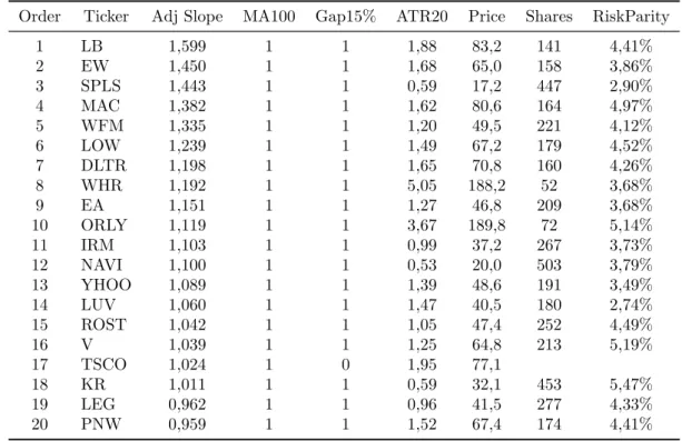
Table I: Ranked constituents S&P500 at 07/01/2015
Filter: S&500 index>MA(200)→OK
Order Ticker Adj Slope MA100 Gap15% ATR20 Price Shares RiskParity 1 LB 1,599 1 1 1,88 83,2 141 4,41% 2 EW 1,450 1 1 1,68 65,0 158 3,86% 3 SPLS 1,443 1 1 0,59 17,2 447 2,90% 4 MAC 1,382 1 1 1,62 80,6 164 4,97% 5 WFM 1,335 1 1 1,20 49,5 221 4,12% 6 LOW 1,239 1 1 1,49 67,2 179 4,52% 7 DLTR 1,198 1 1 1,65 70,8 160 4,26% 8 WHR 1,192 1 1 5,05 188,2 52 3,68% 9 EA 1,151 1 1 1,27 46,8 209 3,68% 10 ORLY 1,119 1 1 3,67 189,8 72 5,14% 11 IRM 1,103 1 1 0,99 37,2 267 3,73% 12 NAVI 1,100 1 1 0,53 20,0 503 3,79% 13 YHOO 1,089 1 1 1,39 48,6 191 3,49% 14 LUV 1,060 1 1 1,47 40,5 180 2,74% 15 ROST 1,042 1 1 1,05 47,4 252 4,49% 16 V 1,039 1 1 1,25 64,8 213 5,19% 17 TSCO 1,024 1 0 1,95 77,1
18 KR 1,011 1 1 0,59 32,1 453 5,47% 19 LEG 0,962 1 1 0,96 41,5 277 4,33% 20 PNW 0,959 1 1 1,52 67,4 174 4,41%
VAMS captures momentum through an exponential regression method provided
by Clenow (2015). This momentum measurement gives each stock a certain slope
dimension. The higher the slope, the higher momentum the stocks exhibits. In
order to minimize the inherent stock risk, we perform a volatility adjustment in the
slope using the exponential regression coefficient of determination R2. A detailed
explanation of this momentum methodology is provided later in this chapter.
As an example, we present in Table I the top ranked 20 stocks of the S&P500
constituents, for the date 07/01/2015. These are sorted by momentum adjusted
slope. In this table we provide for each constituent their others main characteristics
discussed so far: risk parity position sizes, checking if stock is trading below its
SMA(100)5, disclosing if there is a gap in excess of 15%, and checking if S&P500
5
3.1. The strategy rules
index is trading below its SMA(200).
• Construct portfolio using ranking list.
Relying in the information compiled in tables such as the one presented in table I,
we can begin constructing the portfolio. We start from the top of our ranking list
until running out of cash. This aggregates, for the analyzed date t, the portfolio with the highest adjusted momentum effect.
• Rebalance portfolio every week. In 20% strongest stocks, above
SMA(100) and no gap in excess of 15%.
The rank presented in table I will fluctuate every day, reflecting the price oscillations
of the S&P500 constituents acquire over time. Therefore, we need to check if our
portfolio stocks are still fulfilling the criteria needed for them to stay. This criteria
is keep being a stock with high adjusted volatility momentum.
After we enter a position, we need to give it a little space to move, avoiding too
much trading activity and preventing selling good performance stocks too early.
Thus, to perform a portfolio rebalance, each stock in the portfolio must be in the
20% top adjusted volatility momentum S&P500 constituents, otherwise we sell it.
This means that we keep a stock while it remains one of strongest.
We recall that is only allowed to buy new positions if the index trades above is
SMA(200), but we will let stay in the portfolio the already opened positions, as
long as they keep showing high momentum performance. This helps avoiding selling
perfectly good performance stocks just because the index is trading lower. However,
to prevent continuing in the portfolio stocks moving down, we need to set a filter.
We use the moving average filter SMA(100). If a stock starts trading below its 100
day moving average, SMA(100) we deploy a selling order. The same applies if a gap
move, up or down, larger than 15% occurs.
• Rebalance positions, considering changes in volatility every month.
Rebalancing our position size through time is very important. This need results
3.1. The strategy rules
to rebalance our portfolio, otherwise we will be unbalanced in terms of risk. We
proceed this task on a monthly basis to avoid incurring high trading costs.
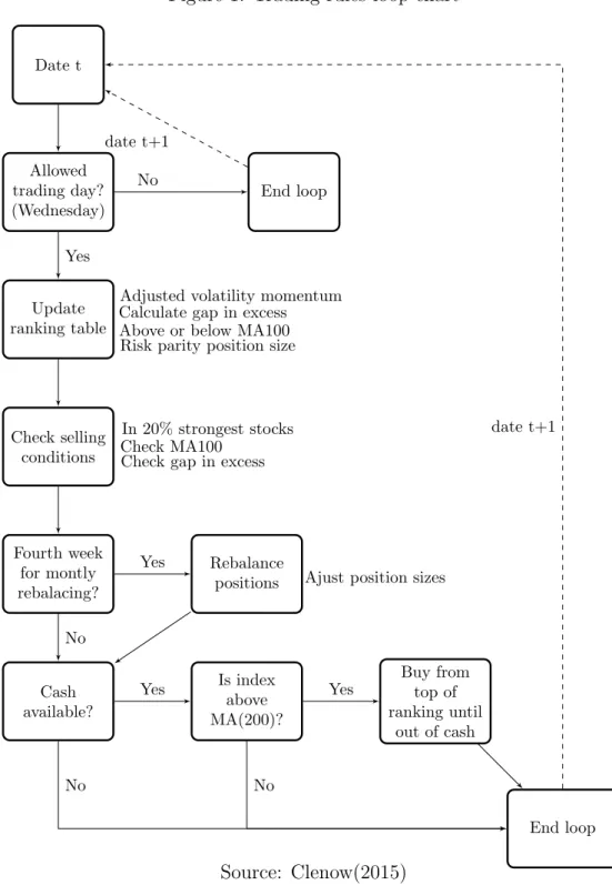
The flowchart presented in Figure 1 aggregates all trading rule information, and how
to logically group them. Please see Clenow (2015)(pp.103). The structure displayed
is used as rational to create an automatized process.
Figure 1: Trading rules loop chart
Date t
Allowed trading day? (Wednesday)
End loop
Update ranking table
Check selling conditions
Fourth week for montly rebalacing?
Rebalance positions
Cash available?
Is index above MA(200)?
Buy from top of ranking until
out of cash
End loop No
date t+1
Yes
Yes No
Yes Yes
No No
date t+1 Adjusted volatility momentum
Calculate gap in excess Above or below MA100 Risk parity position size
In 20% strongest stocks Check MA100
Check gap in excess
Ajust position sizes
3.2. Volatility adjusted momentum process
3.2
Volatility adjusted momentum process
The core scope of VAMS investment is to capture the momentum effect prevailing
in S&P500 stocks. However, momentum by itself only measures the stock recent
performance. It does not take into account the stock volatility, which measures the
returns degree of dispersion as stated by Brownlees and Engle (2010). Therefore,
for any given point in time, we will take into consideration both the momentum and
the volatility when creating our portfolio constituents.
First, we have to find a way of measuring momentum in a stock historical price
series. Fabozzi et al. (2010) declare that a possible method to measure momentum
is using the mathematical concept of linear regression, as denoted in the following
expression;
yi =α+βxi+εi , (3.1)
where yi represents the stock price, xi denotes time expressed in days, α is the
intercept value, β is the slope and ε is the error. Linear regression is a method of
fitting a line over a series of prices, where the resulting line will be the best linear
fit to the price data, minimizing the least squared errors. The slope of that line give
us the direction of the stock price. The linear regression slope on a daily price series
is the same as calculating the average incline or decline per day over the same time
period.
However, this linear slope will be expressed in currency units, and consequently
can’t be used to compare the momentum between stocks. A slope of a stock quoting
at $100 has a complete different magnitude of slope from a stock quoting at $10.
This is why Clenow (2015) suggests using exponential regression as measurement of
momentum, instead of linear regression. The exponential slope give us the average
percentage move a stock is expected to acquire per trading day. This allow us
to compare the slopes, i.e, momentum, among different stocks. The greater the
exponential slope presented by a stock, the stronger the momentum is.
equa-3.2. Volatility adjusted momentum process
tion 3.1. Considering the following exponential model;
yi =αeβxi , (3.2)
taking the natural log in both sides of the equation, we have the following equivalent
equation in the form of a linear regression model, commonly named the log-linear model, which is formally represent as follows;
lnyi =δ+βxi+εi , (3.3)
where α = eδ. The literal interpretation of the estimated coefficient β is that a
one-unit increase in xi will produce an expected increase in lnyi of β. In terms of
yi itself, this means that the expected value of yi is multiplied byeβ.6
Slope can then be easily calculate by a linear regression line (considering the log-linear model) through a set of given points using the following expression:
β =
Pn
i=1(xi−x)(ln¯ yi−ln ¯y)
Pn
i=1(xi−x)¯ 2
, (3.4)
Where the values of ¯x and ln ¯y are the sample means (the averages) of the known
x′s and the known lny′s.
In this work, we consider the past 90 trading days in Equation 3.4, for slope
cal-culations. This 90 days term represents a medium term period of 4.5 months for
past stocks return. Clenow (2015) shows the robustness of the exponential
regres-sion model in capturing momentum for this period, achieving good results. This
is within the range 3- to 12 month holding period referred by Jegadeesh and
Tit-man (1993) as showing momentum prevalence. Since regression slopes are often
very small numbers, for numerical practical reasons, we annualize the stock slope as
follows:
βannualized =e250.βdaily −1 , (3.5)
Now that we have presented how to measure the momentum effect in our investment
6
For small values ofβ, we can approximately assumeeβ≈1 +β. This means that 100.βis the
expected percentage change inyi for a unit increase in xi. For instance, if β =.06, e.
06
≈1.06, then a 1-unit change inxi corresponds to (approximately) an expected increase inyi of 6%. This
3.2. Volatility adjusted momentum process
strategy, we need to adjust it for volatility. This adjustment is done multiplying the
annualized exponential regression slope,β, by the coefficient of determination, R2.7
The higher the volatility, the worse the punishment through slope adjustment. The
result of this product, known as volatility adjusted momentum,βadj, is used to rank
the S&P500 constituents.
As previously showed in Table I, those higher ranked, i.e, displaying higherβadj are
the first in line to be invested.
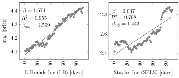
The graphs presented in Figure 2 show two examples of the volatility adjusted
momentum process, for a certain date t.
SPLS presents the strongest momentum, since its β achieves the higher number
(βSP LS = 2.037 vs βLB = 1.674). However, it also exhibits the highest volatility as
consequence of the coefficient of determination, R2, being the lowest among both
stocks (R2
SP LS = 0.708 vs R2LB = 0.955). This means that the ranking, represented
by the volatility adjusted momentum beta, βadj, is more punished in SPLS than in
LB (βSP LS
adj = 1.443 vsβadjLB = 1.559). Prices are less erratic in LB being the uptrend
smoother than the one presented by SPLS.
Figure 2: Volatility adjusted momentum examples
0 20 40 60 80
4.1 4.2 4.3
4.4 β = 1.674 R2 = 0.955
βadj = 1.599
L Brands Inc (LB) [days]
ln
yi
[p
ri
ce
]
0 20 40 60 80
2.4 2.6
2.8 Rβ2= 2= 0.708.037
βadj = 1.443
Staples Inc (SPLS) [days]
7
This coefficient will take values between 0 and 1. An R2
of 1 indicates that the regression line perfectly fits the data, and the lowerR2
is, the worse the fit is. Thus, a stock exhibiting lower volatility will present a higherR2
, while a more volatile stock will get a lowerR2
3.3. Risk parity positions and rebalancing process
3.3
Risk parity positions and rebalancing process
3.3.1
Position size
The portfolio asset allocation method is very important, because when determining
position size, we are actually allocating risk. If all stocks have identical volatility, an
equally weighted positioning size method would be satisfactory. However, volatility
among stocks differs and we use a risk parity asset allocation process. This means
we distribute the same risk per portfolio position. Thus, for a certain date t, the amount of shares to be invested and guarantee risk parity for each stock, is given
by the following equation;
Sharesit= AccountV aluet∗RiskF actor AT Ri
t
, (3.6)
where AccountValue is the amount of money we have in our disposal at time t,
Riskfactor represents the daily impact for the stock in the overall portfolio andAT R states for average true range (ATR), which is an indicator that measures volatility.
For example, if we setriskfactor equal to 0.001, then we are targeting a daily impact in the portfolio of 0.1%, or 10 basis points. The lower this number is, the higher
the number of stocks we will have in our portfolio. Therefore, diversification will
increase as we lower theriskfactor.
ATR gives us ann-day smoothed moving average (SMMA) of the true range values, being the true range the maximum of day’s high to low or move from previous day.
True range can be obtained by using the following expression;
T R=max[(high−low), abs(high−closeprev), abs(low−closeprev)] , (3.7)
The ATR at the moment of timet can be generically calculated as follows;
AT Rt=
AT Rt−1∗(n−1) +T Rt
n , (3.8)
3.3. Risk parity positions and rebalancing process
first ATR value to be considered is calculated using the arithmetic mean formula;
AT R= 1 n
n
X
i=1
(T Ri) , (3.9)
Considering this risk based asset allocation heuristic approach we can aim for a risk
parity portfolio, where every stock as an equal theoretical chance to impact our
strategy overall portfolio.
3.3.2
Position rebalancing
Since the ATR indicator can easily capture the volatility dynamics, we will use the
ATR based formula presented in equation 3.6 to rebalance our position every month
(δ = 20).
Sharesit+δ = AccountV aluet+δ∗RiskF actor AT Ri
t+δ
, (3.10)
This means that in a monthly basis, we change the number of shares of each stock,
in order to obtain a steady risk allocation over time. Please pay attention to the
fact that theAccountValue changes through time, impacted by the performance of all portfolio position over time.
In order to prevent doing many small trades when rebalancing, we set a minimum
value of 10%8 in shares variation between months.
8
Chapter 4
Data and methodology
In this chapter we describe the data and the methodology we used for constructing
the volatility adjusted momentum strategy (VAMS) previously defined.
4.1
Data
We draw your attention to the fact that our strategy comprises only stocks. Other
financial assets such as bonds, commodities or derivatives are not taken into
con-sideration. In order to significantly reduce the amount of data to be analyzed, we
consider the assumption of not existing trading costs1. Our main source for stock
data is Yahoo Finance2. We employ their free database website to download and
compile historical prices for all the index components. This website has the massive
advantage of providing historical price time-series accounting to cash dividends and
splits. This is highly important because to get a correct picture of the actual
finan-cial development of a share price, the series need to be adjusted back in time, and
Yahoo Finance allows it.
The index we consider as benchmark and as source of picking our momentum
strat-egy stocks is the S&P5003. We collect the S&P500 historical index components
membership and index delisted stocks by using a Bloomberg4 terminal.
The data-set spans a eleven years period, between January 2005 to December 2015,
1
In real world trading costs can’t be ignored. Later in our project we conduct a stress test to VAMS with the propose of measuring the impact of these in our portfolio.
2
http://finance.yahoo.com/
3
The S&P500 index is itself a momentum index, therefore by definition this index is essentially a very long term investment momentum strategy. A stock to be considered for inclusion in the SP&500, market capitalization must be over 5.3 billion dollars. This means that a certain stock is part of the index because it had had a strong price development in the past. When a stock leaves the index, it’s usually because it had poor price performance and dropped below the market cap requirement.
4
4.2. Methodology
comprising a total of 574 weeks. This translates into constructing a portfolio in
January 2005 and manage it according to VAMS until December 2015. We also
study performance for other holding periods. These consist in similarly constructing
a portfolio in the beginning of all the subsequent years until Dec 2015. For example,
Jan 2006 to Dec 2015, Jan 2007 to Dec 2015, etc. Thus, a total of 11 backtests are
performed to VAMS.
In order to perform and backtest our strategy we collect historical daily stock prices
on a weekly basis. We analyzed over 280000 stock time-series and performed over
15000 trades distributed through the 11 main backtests we performed. An average
of 4.6 trades per week.
We provide further confirmation regarding VAMS effectiveness by carrying out a
out-of-sample test, from January 2016 to July 2016. This comprehends a total of
28 weeks.
4.2
Methodology
Our main objective is to capture the momentum effect of a large set of stocks, and
allocate our investment in the stocks showing the strongest momentum performance.
Therefore, we need to find a proper way to rank the S&P500 stock constituents,
considering all of our strategy features and particularities. The flowchart presented
in Figure 3 illustrates the overall implementation process step by step. As VAMS
is fully automatized this rational is not time-depended, i.e. it can be used for any
given time interval as long as Yahoo and Bloomberg databases are accessible.
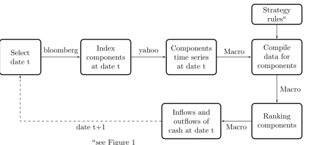
The steps to proceed are as follows, being also illustrated in Figure 3;
• The first step comprehends choosing a certain date t for which we want to set up our portfolio.
• Secondly, we consider the index components, for the previously selected date
t, as potential stocks to be included in our portfolio.
• Next, after knowing which index stocks should be considered, we access to
4.2. Methodology
• According to the VAMS rules described in section 3.1, compile all the
infor-mation for every index components.
• Considering all the compiled information we rank all the index components by
momentum.
• Create, delete or rebalance positions according to the new inflows and outflows
of cash necessities.
Figure 3: VAMS implementation flowchart
Select date t
Index components
at date t
Components time series
at date t
Compile data for components
Strategy rulesa
Ranking components Inflows and
outflows of cash at date t
bloomberg yahoo Macro
Macro
Macro date t+1
Chapter 5
Results
In this chapter we present the overall results achieved by applying VAMS to the
S&P500 index. We compare the strategy’ performance with the index itself, in terms
of absolute returns, annualized returns, risk-adjusted returns (Sharpe ratio) and
value-at-risk (VaR), as well as descriptive statistics. We also compare drawdowns
performance1.
We study performance for 11 different holding periods, as previously described, being
the longest from Jan 2005 to Dec 2015.
Later, we realize a stress test to VAMS. This test consists in accounting trading
costs in VAMS, and see how performance is affected. Multiple possibilities, per
stock trade, are considered.
Finally, in order to check VAMS robustness, we perform a out-of-sample process.
The period selected goes from Jan 2016 to Jul 2016. Even though a longer
out-of-sample period would have been preferable this will be helpful on guiding us on how
well the system might perform with new data.
5.1
VAMS vs benchmark performance
We start by presenting, in Table II, the overall results VAMS achieved for the 11
years investment period, and compare it to the outcomes obtained by the benchmark.
The VAMS approach outperforms the index, with absolute returns 52% higher
(179.5% vs 118.0%). In annualized terms the values are 9.8% and 7.4%, for the
VAMS and the index respectively. In terms of risk-adjusted returns, VAMS performs
also better with a Sharpe ratio of 0.64 vs 0.42 of the S&P500. The huge difference
1
5.1. VAMS vs benchmark performance
Table II: 11 years VAMS performance (Jan 2005 - Dec 2015)
2005-15 Period
VAMS S&P500
Absolute Returns 179,5% 118,0%
Annualized Returns 9,8% 7,4%
Sharpe Ratio 0,63 0,42
Max. 1Y Drawdown -18,6% -48,1%
Historical VaR 95% -0,033 -0,036
Gaussian VaR 95% -0,032 -0,037
between 1 year maximum drawdowns, and inferior VaR2 values, corroborate that
VAMS allow for a better risk control than passively investing in the S&P500.
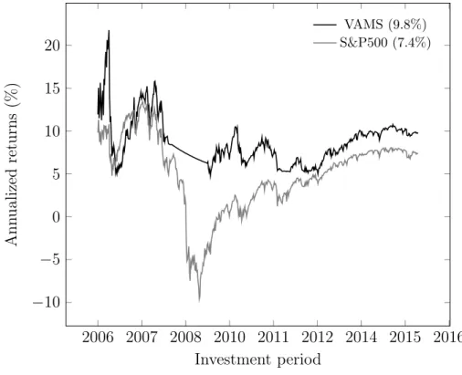
Figure 4 shows how absolute returns progressed during the eleven years investment
period, while Figure 5 illustrates the development of annualized returns.
Figure 4: Absolute returns dynamic performance - Jan 2005 to Dec 2015
2005 2006 2007 2009 2010 2011 2013 2014 2015
−50
0 50 100 150 200
Investment period
Ab
so
lu
te
re
tu
rn
s
(%
)
VAMS (179.5%) S&P500 (118%)
In terms of absolute returns, VAMS also outperforms the index. From Figure 4 it
is clear that our approach exceeds the index almost the entire investment period,
except for a small time period in the beginning years. It is also evident the capability
2
5.1. VAMS vs benchmark performance
of VAMS to avoid major market turns, such as the market meltdown occurred in
the 2008-09 financial crisis. For further information in terms of each year relative
gains, see Table VIII in Appendix A. To consult VAMS constituents over time at
the beginning of each year, see Table IX in Appendix A.
The annualized returns progression over time, exhibited in the Figure 5, helps
sup-porting VAMS better performance. Before stabilizing near the 10% value, our
ap-proach produces an annualized return always positive and above 5%. The index
exhibits most of the time lower and more volatile values.
Figure 5: Annualized returns dynamic performance - Jan 2005 to Dec 2015
2006 2007 2008 2010 2011 2012 2014 2015 2016
−10
−5
0 5 10 15 20
Investment period
An
n
u
al
iz
ed
re
tu
rn
s
(%
)
VAMS (9.8%) S&P500 (7.4%)
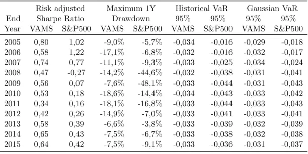
More insights can be withdraw from Table III, specifically the apparent lower risk
VAMS shows when compared to the index. The majority of the years show in terms
of Sharpe ratio, maximum 1Y drawdown and VaR, better performance as exhibit
higher values. VaR calculations consider two quantitative approaches, the historical
VaR and gaussian (parametric) VaR, for 95% confidence levels3. VAMS also presents
3
5.1. VAMS vs benchmark performance
more coherent values through the years, while the index is more inconsistent.
Table III: Risk indicators evolution by year - Jan 2005 to Dec 2015
Risk adjusted Maximum 1Y Historical VaR Gaussian VaR
End Sharpe Ratio Drawdown 95% 95% 95% 95%
Year VAMS S&P500 VAMS S&P500 VAMS S&P500 VAMS S&P500
2005 0,80 1,02 -9,0% -5,7% -0,034 -0,016 -0,029 -0,018
2006 0,58 1,22 -17,1% -6,8% -0,032 -0,016 -0,032 -0,017
2007 0,74 0,77 -11,1% -9,3% -0,033 -0,025 -0,034 -0,024
2008 0,47 -0,27 -14,2% -44,6% -0,032 -0,038 -0,031 -0,041
2009 0,56 0,07 -7,6% -48,1% -0,033 -0,044 -0,031 -0,043
2010 0,53 0,18 -18,6% -14,4% -0,034 -0,043 -0,033 -0,042
2011 0,34 0,16 -18,1% -16,8% -0,033 -0,044 -0,033 -0,043
2012 0,42 0,26 -14,9% -7,0% -0,033 -0,041 -0,033 -0,041
2013 0,58 0,39 -6,6% -3,8% -0,033 -0,039 -0,032 -0,039
2014 0,65 0,43 -7,5% -6,7% -0,033 -0,038 -0,032 -0,038
2015 0,64 0,42 -7,5% -9,1% -0,033 -0,036 -0,031 -0,037
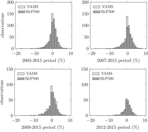
Next, in Table IV we compile the main descriptive statistics, for both VAMS and
the S&P500, while histograms in Figure 6 give some extra insights. The presented
statistics concern not only the 11 years investment period covered so far but also 3
other important investment horizons. The 2007-15 period which comprehends the
beginning of the financial crisis, the 2009-15 period that concerns the financial crisis
ending and lately, the considerable 2012-15 bull market.
VAMS exhibits better performance in terms of annualized mean returns in all cases,
excepting for the 2009-15 period. The standard deviation, as well as the absolute
values of maximum and minimum weekly returns, are in almost situations higher for
the S&P500. This might be an indication of higher volatility presence in the index.
Both VAMS and the index present negative skewness. VAMS always presents a value
of skewness higher than -1, which allows us to consider its returns as moderately
skewed. On the other hand, the index returns half of times present a skewness
lower then -1, making it highly skewed. This implies that negative returns are more
common when investing in the index.
VAMS kurtosis are lower than 3. This indicates that our approach distribution
produces fewer and less extreme outliers than the normal distribution. This situation
5.1. VAMS vs benchmark performance
Table IV: VAMS and S&P500 descriptive statistics
2005–2015 Ann. Mean Ann. St.Dev Skewness Kurtosis Minimum Maximum VAMS 9,33% 14,67% -0,80 2,06 -8,99% 5,56% S&P500 7,28% 16,73% -1,32 8,44 -17,42% 9,56%
VAMS and S&P500 correlation = 0,6068
2007–2015 Ann. Mean Ann. St.Dev Skewness Kurtosis Minimum Maximum VAMS 10,31% 15,01% -0,78 2,14 -9,68% 5,47% S&P500 6,24% 18,02% -1,28 7,43 -17,42% 9,56%
VAMS and S&P500 correlation = 0,6048
2009–2015 Ann. Mean Ann. St.Dev Skewness Kurtosis Minimum Maximum Strategy 11,35% 15,09% -0,75 1,87 -9,72% 5,43%
S&P500 13,75% 16,24% -0,59 3,40 -11,65% 9,56% Strategy and S&P500 correlation = 0,7147
2012–2015 Ann. Mean Ann. St.Dev Skewness Kurtosis Minimum Maximum Strategy 17,47% 14,20% -0,63 1,28 -6,80% 5,26%
S&P500 13,99% 11,68% -0,61 1,89 -6,88% 3,98% Strategy and S&P500 correlation = 0,8402
Figure 6: VAMS vs S&P500 weekly returns histograms - Multiperiods
−20 −10 0 10
0 50 100 150 200
2005-2015 period (%)
ob se rv at io n s VAMS S&P500
−20 −10 0 10
0 50 100 150 200
2007-2015 period (%)
VAMS S&P500
−20 −10 0 10
0 50 100 150
2009-2015 period (%)
ob se rv at io n s VAMS S&P500
−20 −10 0 10
0 50 100 150
2012-2015 period (%)
5.1. VAMS vs benchmark performance
distribution generates a very high kurtosis because it produces more outliers than
the normal distribution. The ”heavy tails” presence can easily be confirmed when
checking the index histograms in figure 6.
It is important to notice that VAMS returns are moderately positively correlated
(+0.6048 to +0.6068) to those presented by the index in the periods that cover
the 2008-09 financial crisis. The correlation substantially increases in the years
after the crisis (+0.7147 to +0.8402). A positive correlation is expected since our
portfolio constituents are all selected from the S&P500. However, the discrepancy
in correlation values, before and after the crisis, indicates the capability of VAMS
outperform the index in market turmoils. Correlation decreases in market turn
downs because VAMS stops investing while the index keeps moving.
Table V provides a complete overview of VAMS performance versus the one obtained
by the S&P500. The table background is presented in two different colors. In case
of being displayed in light gray, the S&P500 index performed better, otherwise it
is VAMS that has outperformed. More detailed information can be consulted in
Appendix A.
In 9 of the 11 backtests, VAMS seems to outperform the index, presenting only worst
outcomes in the 2009-15 and 2010-15 tests. These results make us strongly believe
that in the long run VAMS is expected to outperform the benchmark S&P500,
specially in terms of reducing portfolio risk and avoiding exposure to major market
5.1. VAMS vs benchmark performance
Table V: Strategy and benchmark main results
2005-15 Period 2006-15 Period 2007-15 Period
VAMS S&P500 VAMS S&P500 VAMS S&P500
Absolute Returns 179,5% 118,0% 169,5% 98,6% 153,4% 75,6%
Annualized Returns 9,8% 7,4% 10,4% 7,1% 10,9% 6,5%
Sharpe Ratio 0,63 0,42 0,65 0,39 0,69 0,35
Max. 1Y Drawdown -18,6% -48,1% -19,4% -48,1% -19,4% -48,1%
Historical VaR 95% -0,033 -0,036 -0,033 -0,038 -0,034 -0,040
Gaussian VaR 95% -0,032 -0,037 -0,033 -0,038 -0,032 -0,040
2008-15 Period 2009-15 Period 2010-15 Period
VAMS S&P500 VAMS S&P500 VAMS S&P500
Absolute Returns 121,8% 68,2% 121,8% 162,5% 90,1% 104,6%
Annualized Returns 10,4% 6,7% 12,1% 14,8% 11,3% 12,7%
Sharpe Ratio 0,70 0,35 0,75 0,85 0,70 0,81
Max. 1Y Drawdown -19,7% -48,1% -19,7% -20,9% -19,7% -16,8%
Historical VaR 95% -0,033 -0,040 -0,033 -0,036 -0,034 -0,034
Gaussian VaR 95% -0,030 -0,041 -0,032 -0,034 -0,033 -0,031
2011-15 Period 2012-15 Period 2013-15 Period
VAMS S&P500 VAMS S&P500 VAMS S&P500
Absolute Returns 79,7% 78,7% 101,8% 75,0% 74,7% 49,7%
Annualized Returns 12,5% 12,4% 19,2% 15,1% 20,5% 14,4%
Sharpe Ratio 0,80 0,82 1,23 1,192 1,35 1,162
Max. 1Y Drawdown -19,0% -16,8% -9,9% -9,1% -8,8% -9,1%
Historical VaR 95% -0,033 -0,027 -0,030 -0,025 -0,027 -0,024
Gaussian VaR 95% -0,031 -0,031 -0,029 -0,024 -0,027 -0,024
2014-15 Period 2015-15 Period All Periods Average
VAMS S&P500 VAMS S&P500 VAMS S&P500
Absolute Returns 29,4% 17,1% 4,7% 3,9% 101,8% 77,4%
Annualized Returns 13,6% 8,4% 4,8% 4,0% 12,3% 9,9%
Sharpe Ratio 0,95 0,64 0,38 0,303 0,80 0,662
Max. 1Y Drawdown -8,6% -9,1% -8,3% -9,1% -15,5% -25,7%
Historical VaR 95% -0,026 -0,026 -0,027 -0,022 -0,031 -0,032
5.2. VAMS trading costs stress test
5.2
VAMS trading costs stress test
So far in our study, we have not considered the existence of trading costs in VAMS
performance analysis. This was an assumption that reduced considerably the amount
of data to be analyzed. However in the real world trading costs exist and cannot be
ignored. We now present a stress test that measures the impact these costs would
have done to our portfolio absolute returns, considering an initial $100.000 account,
in the 11 years backtest. From Jan 2005 to Dec 2015, which is the longest time
period studied.
Trading costs are the brokerage commission payed to a brokerage firm for executing
our trades. Each stocks buy or sell incurs on fee that must be deducted from our
portfolio account. Since the fee value differs among brokers, we consider 4 distinct
values: 4$, 6$, 8$ and 10$ per trade.
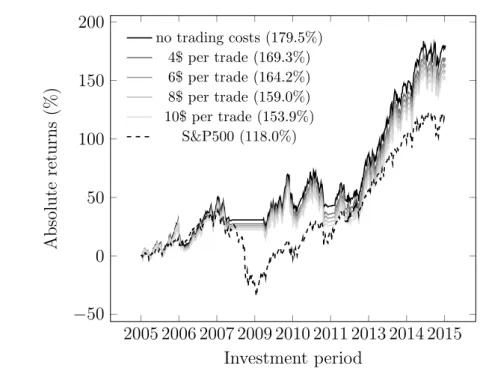
During the 11 years, around 2700 trades were triggered, and Figure 7 shows the
degree of susceptibility VAMS has to these. In the worst scenario, 10$ per trade,
absolute returns are only 85% of those achieved by base scenario. In the best scenario
returns present a higher value of 94%. Thus, returns can be considerably affected by
trading costs, even though VAMS keeps outperforming the index in every scenario.
Figure 7: Trading costs stress test - Jan 2005 to Dec 2015
2005 2006 2007 2009 2010 2011 2013 2014 2015
−50
0 50 100 150 200
Investment period
Ab
so
lu
te
re
tu
rn
s
(%
)
no trading costs (179.5%) 4$ per trade (169.3%) 6$ per trade (164.2%) 8$ per trade (159.0%) 10$ per trade (153.9%)