OPTIMIZED, AUTOMATED SHIMMING PROCEDURE FOR IMPROVED
EXPERIMENTAL CARDIAC MAGNETIC RESONANCE IMAGING AND
SPECTROSCOPY AT ULTRA-HIGH MAGNETIC FIELDS
by
Cristiano José da Silva Barros Amaral
OPTIMIZED, AUTOMATED SHIMMING PROCEDURE FOR IMPROVED
EXPERIMENTAL CARDIAC MAGNETIC RESONANCE IMAGING AND
SPECTROSCOPY AT ULTRA-HIGH MAGNETIC FIELDS
Thesis presented to
Escola Superior de Biotecnologia
of the
Universidade Católica
Portuguesa
to fulfil the requirements of Master of Science degree in Biomedical
Engineering
by
Cristiano José da Silva Barros Amaral
Place: British Heart Foundation Experimental MR Unit, Wellcome Trust Centre for
Human Genetics, University of Oxford, Oxford, United Kingdom
Supervision: Doctor Jürgen Schneider
III
Resumo
Background: As técnicas de ressonância magnética cardíaca por imagem (MRI) e espetroscopia (MRS) são ferramentas usadas para caraterizar, de forma não invasiva, modelos de rato com doenças cardíacas humanas. As experiências são tipicamente conduzidas em sistemas de Ressonância Magnética (MR) equipados com magnetos de elevada intensidade (≥ 7 Tesla). Um requisito fundamental da MR é a homogeneidade do campo magnético estático, B0 (Grutter, 1993), e
as flutuações (inomogeneidades) do campo magnético principal na região de imagem devem ser menores a três partes por milhão (3 ppm). Inserindo uma amostra aumenta-se a inomogeneidade do campo (devido a diferentes graus de magnetização ao longo da amostra como resposta a B0
("suscetibilidade magnética")), a qual necessita de ser compensada (Crijns et al, 2011; Koch et al, 2006). Homogeneizar (shimming) o campo magnético estático é uma tarefa crucial em qualquer experiência de MR para maximizar a resolução e a razão entre sinal e ruído. Isto é particularmente importante em campos magnéticos de elevada intensidade devido à dependência linear da suscetibilidade magnética com B0. O ajuste manual das bobinas de shim é laborioso e subjetivo. Para
além disso, este processo é particularmente desafiante onde vários tecidos (por exemplo, osso, fluxo de sangue, entre outros) estão numa vizinhança próxima dentro do tórax, tendo cada um diferentes suscetibilidades magnéticas e movimentos relativos. Métodos automáticos de shimming, como o FASTMAP ou FASTERMAP (Shen et al, 1997), estão experimental e clinicamente bem estabelecidos no tecido cerebral mas falham no coração devido à fase de sinal mal definida de MR, particularmente no interior dos ventrículos. Com base numa técnica previamente implementada para o cérebro humano, foi investigada a implementação de uma nova abordagem para corações de ratos, in vivo, capaz de homogeneizar B0 na região de interesse, com uma forma aleatória.
Objetivo: O objetivo deste projeto é investigar os parâmetros ótimos de digitalização e pós-processamento, por forma a otimizar e alcançar um procedimento automático de shimming, potenciando, assim, as técnicas de MRI e MRS cardíacas.
Métodos: Diversos ratos (n=5) foram submetidos à técnica de MR, realizada num magneto horizontal de 9.4 Tesla (T). A aquisição de imagem foi conduzida através de sequências rápidas echo variando os seguintes parâmetros: resolução, compensação de fluxo (on / off), orientação (short-axis / axial) e dimensão (multi-cortes 2D vs 3D). Três diferentes configurações de bobinas de shim foram investigadas e a sequência ótima de MR foi avaliada.
Resultados: O nível de 17% de threshold demonstrou ser aceitável para a remoção das discontinuidades de fase. A análise quantitativa do desempenho das diferentes abordagens de phase unwrapping mostrou que a abordagem 3D é a mais eficaz na resolução das discontinuidades de fase presentes nos mapas de campo. A aplicação de orientação axial, os dados de maior resolução, a ausência de compensação de fluxo e a introdução de bobinas de shim de maiores ordens demonstraram um peso significativo na redução das inomogeneidades de B0, quando aplicados.
Conclusões: Este projeto permitiu estabelecer parâmetros ótimos de aquisição e opções de pós-processamento que melhoram a homogeneidade de B0, importantes na validação de futuros estudos
V
Abstract
Background: Cardiac magnetic resonance imaging and spectroscopy are tools to non-invasively characterize rodent models of human heart disease. The experiments are typically carried out on dedicated MR systems equipped with ultra-high field magnets (≥ 7 Tesla). One fundamental requirement of MR is the homogeneity of the static magnetic field B0 (Grutter, 1993), and fluctuations
of the main magnetic field (B0 inhomogeneities) within the scan region should be less than three parts
per million (3 ppm). Inserting a sample inherently increases the field inhomogeneity (due to different degree of magnetization across the sample in response to the B0 field (“magnetic susceptibility”)),
which needs to be compensated for (Crijns et al, 2011; Koch et al, 2006). Homogenizing (i.e. shimming) the static magnetic field is crucial for any MR experiment in order to maximize resolution and signal-to-noise. This is particularly important at ultra-high magnetic fields due to linear dependence of magnetic susceptibility. Adjusting the three linear and typically up to 14 higher order shims manually is laborious and subjective. Moreover, this process is particularly challenging where various tissues (i.e. heart and skeletal muscle, bone, lungs and flowing blood) are in close vicinity within the chest, each having different magnetic susceptibilities and relative motions. Auto-shim methods such as FASTMAP or FASTERMAP (Shen et al, 1997), are clinically and experimentally well established in brain tissue, but inevitably fail in the heart due to the ill-defined phase of the MR-signal, particularly inside the ventricles. Based on a technique, previously applied to human brain – implemented a novel approach for the application to mouse hearts in vivo, that is able to homogenize the B0-field in an arbitrarily shaped, but connected region of interest.
Aim: The aim of this project is to investigate optimal scan parameters and post-processing approach to optimize and advance an automated shimming procedure for improved experimental cardiac magnetic resonance imaging and spectroscopy at ultra-high magnetic fields.
Methods: Mice (n = 5) underwent MR experiments carried out in a 9.4 Tesla (T) horizontal magnet. The image acquisition was performed using fast gradient echo sequences varying the following parameters: resolution, flow compensation on / off, orientation (short-axis / axial), and dimension (2D multislice vs 3D). Three different shim coils’ configurations (shim coils up to the third order) were investigated and optimal MR sequence was assessed.
Results: The threshold level of 17% proved to be acceptable for removal of phase discontinuities and hence it was used in subsequent studies. Quantitative analysis of the performance of different phase unwrapping approaches showed that the 3D approach is the most effective in resolving phase discontinuities present in field maps. The application of axial orientation, highest resolution data, absence of compensation flow and the introduction of higher order shim coils showed a significant reduction of B0 inhomogeneities when applied.
Conclusions: This project established optimal acquisition parameters and post-processing options to improve the homogeneity of B0, and will aid the validation process in further follow-up studies.
VII
Acknowledgements
My deepest gratitude goes first to Dr. Jurgen Schneider, who expertly guided me through this journey. I am very thankful for his sympathy, friendship, solidarity, supervision and indispensable help. But above all, I am extremely grateful for the unique opportunity of living the biggest personal and academic challenge so far.
I would like to express my appreciation to Dr. Stefan Neubauer for having forwarded my project request to the British Heart Foundation MR Unit (BMRU) – Wellcome Trust Center for Human Genetics – University of Oxford.
I am most grateful to Dr. Mark Jenkinson for his important contribution during the project and for his willingness to help to overcome some obstacles.
I extend my appreciation to Dr. Jean-Baptiste Cazier for his cooperation, support and valuable suggestions given for future work.
I owe my sincere gratitude to Professor João Paulo Ferreira for his essential help throughout this time.
I am very thankful to Ms. Ana Luísa Silva for her unconditional support and indispensable help.
It is with immense gratitude that I acknowledge the support and help of Dr. Mahon Maguire. I also would like to thank him for his immense sympathy and friendship.
It gives me great pleasure in acknowledging the support and help of my desk mate, Mr. Kyle Caldock.
I sincerely thanks to Dr. Kiterie Faller for her kindness, companionship and help to face the challenge.
I wish to thank Ms. Vicky Thornton for her help and friendship.
I would like to thank Mrs. Lee-Anne Stork for her kindness and for having welcomed me first so well at BMRU.
Thanks also go to Dr. Maélène Lohezic for all support.
In addition, I thank Mr. John Cleland, Mr. Phil Ostrowski and all Christ Church College Football Team for all the entertainment provided during all this time of hard work.
VIII
I would like to give my special and profound thanks to my parents and brothers, whose enthusiasm, encouragement and faith have been particularly helpful. I am extremely grateful for their incredible support.
I also would like to thank Professor Joaquim Agostinho Moreira for his valuable help and patience always addressed to all of my questions.
Lastly, I am indebted to my many friends for being part of my life and for their incredible support.
IX
Contents
Page
Resumo III Abstract V Acknowledgments VII List of figures XIList of tables XIII
List of abbreviations XV Chapter 1 – Background 1.1. Basics of MR 3 1.2. Cardiac MRI 4 1.3. Shimming 4 1.4. Shim-calibration 5 Chapter 2 –Methods 2.1. In vivo setup 9
2.2. MR sequences based on gradient echo sequences 9
2.3. Post-processing 9
2.4. Statistical analysis 10
Chapter 3 – Results
3.1. Optimal threshold 13
3.2. Optimal phase unwrapping approach 14
3.3. Optimal data processing 20
3.4. Optimal MR sequence 20
Chapter 4 – Discussion 31
Chapter 5 – Conclusions and Future Research 35
References 39
Appendix
Appendix A 45
Appendix B 51
XI
List of figures
Page
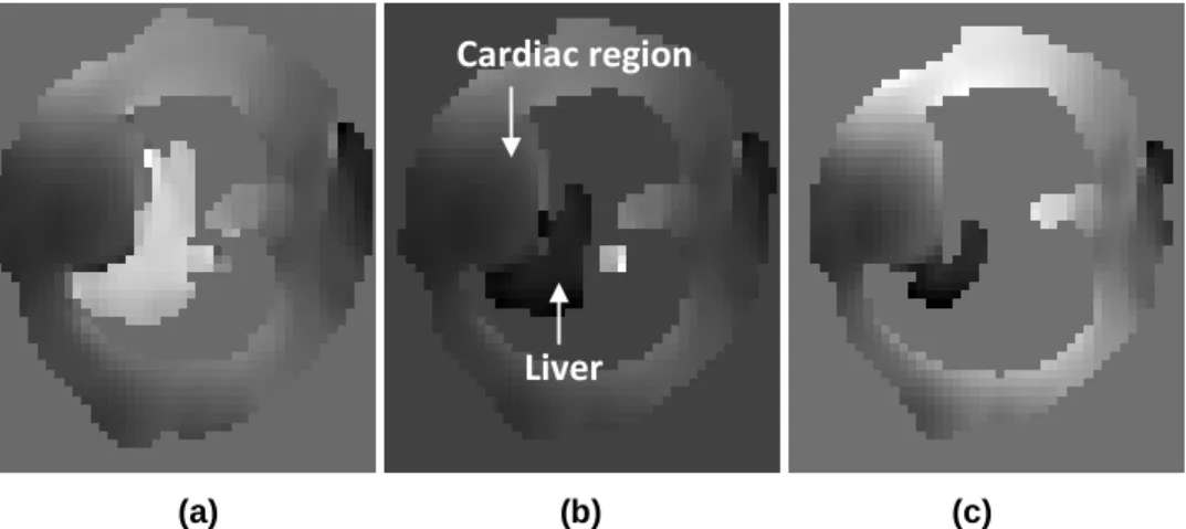
Figure 1. Single dataset representation using three different threshold levels: 10% (a), 17% (b), and 25% (c). The phase discontinuities are presented by the rapid changes in the image greyscale.
13
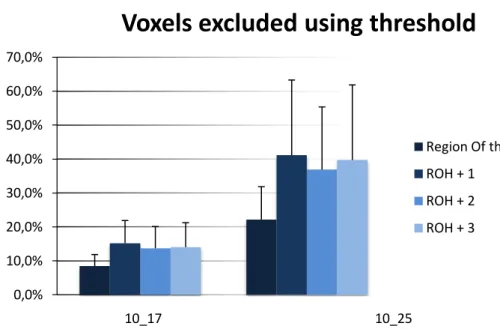
Figure 2. Results for removed voxels caused by the increase of threshold level. To this study all data sets were considered.
14
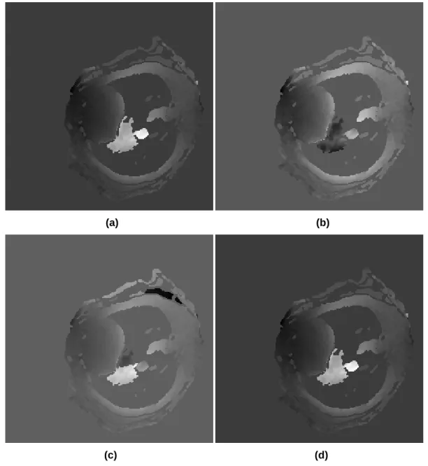
Figure 3. Single dataset representation using the same threshold level (17%) and all options of phase unwrapping algorithm: 2D (a), 2D + RR (b), 3D (c) and 3D + RR (d).
15
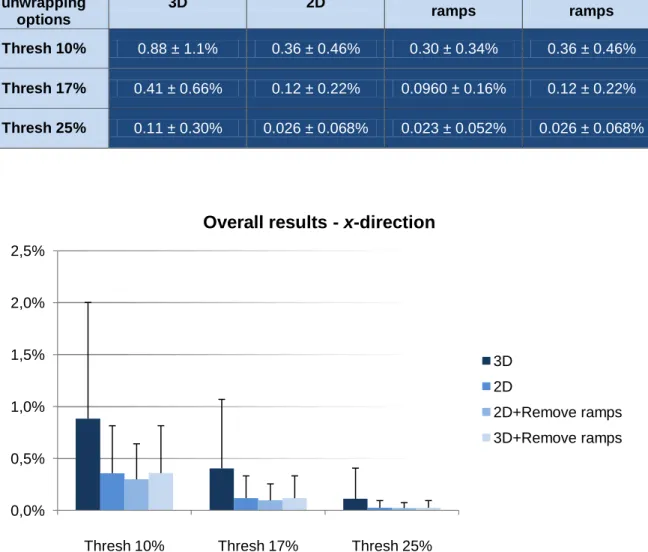
Figure 4. Results of the remaining phase discontinuities after the application of four different phase unwrapping algorithms, based on the x-direction, having into consideration all data sets available.
16
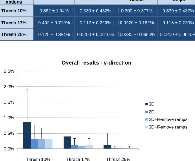
Figure 5. Results of the remaining phase discontinuities after the application of four different phase unwrapping algorithms, based on the y-direction, having into consideration all data sets available.
17
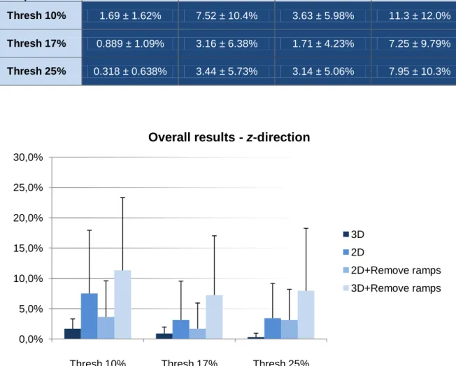
Figure 6. Results of the remaining phase discontinuities after the application of four different phase unwrapping algorithms, based on the z-direction, having into consideration all data sets available.
18
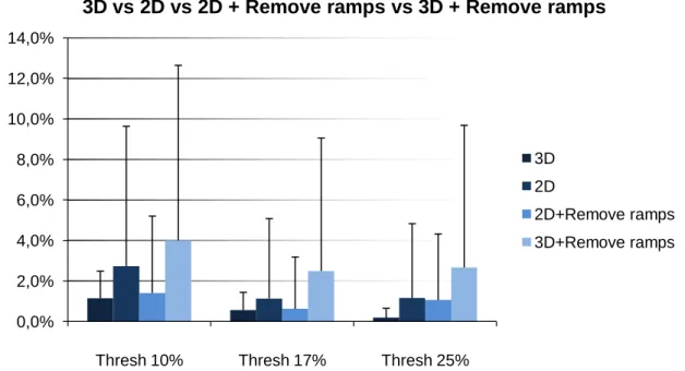
Figure 7. Results of the remaining phase discontinuities after the application of four different phase unwrapping algorithms, based on the x-, y- and z-direction, having into consideration all data sets available.
19
Figure 8. Representation of raw data distribution (above); normal distribution after logarithm transformation of raw data (bottom).
21
Figure 9. Influence of different orientation settings (axial vs short-axis) on residual field measures (log measures).
22
Figure 10. Influence of using or not using flow compensation on residual field measures (log measures).
XII
Figure 11. Influence of different dimension settings (2D vs 3D) on residual field measures (log measures).
24
Figure 12. Influence of different source configurations (e.g. orientation: axial; dimension: 3D; flow compensation: yes; resolution: high) on residual field measures (log measures).
25
Figure 13. Influence of different shim coils’ configurations (up to first order vs up to second order vs up to third order (only simulated)) on residual field measures (log measures).
26
Figure 14. Influence of different resolution settings on residual field measures (log measures).
27
Figure A.1. Results of the remaining phase discontinuities after the application of four different phase unwrapping algorithms, based on the x-direction, having into consideration all 2D data sets available.
45
Figure A.2. Results of the remaining phase discontinuities after the application of four different phase unwrapping algorithms, based on the y-direction, having into consideration all 2D data sets available.
46
Figure A.3. Results of the remaining phase discontinuities after the application of four different phase unwrapping algorithms, based on the z-direction, having into consideration all 2D data sets available.
47
Figure A.4. Results of the remaining phase discontinuities after the application of four different phase unwrapping algorithms, based on the x-direction, having into consideration all 3D data sets available.
48
Figure A.5. Results of the remaining phase discontinuities after the application of four different phase unwrapping algorithms, based on the y-direction, having into consideration all 3D data sets available.
49
Figure A.6. Results of the remaining phase discontinuities after the application of four different phase unwrapping algorithms, based on the z-direction, having into consideration all 3D data sets available.
50
Figure C.1. Influence of different shim coils’ configurations (up to first order vs up to second order) on residual field measures (log measures).
XIII
List of tables
Page
Table 1. Mean and standard deviation measures for removed voxels caused by the increase of threshold level. To this study all data sets available were considered.
13
Table 2. Mean and standard deviation measures for remaining phase discontinuities after the application of four different phase unwrapping algorithms, based on the x-direction, having into consideration all data sets available.
16
Table 3. Mean and standard deviation measures for remaining phase discontinuities after the application of four different phase unwrapping algorithms, based on the y-direction, having into consideration all data sets available.
17
Table 4. Mean and standard deviation measures for remaining phase discontinuities after the application of four different phase unwrapping algorithms, based on the z-direction, having into consideration all data sets available.
18
Table 5. Mean and standard deviation measures for remaining phase discontinuities after the application of four different phase unwrapping algorithms, based on the x-, y- and z-direction, having into consideration all data sets available.
19
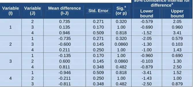
Table 6. Statistical analysis comparing the (non-)utilization of RPD and/or RSVP options; GLM method and Bonferroni post-Hoc test application to the first data set.
20
Table A.1. Mean and standard deviation measures for remaining phase discontinuities after the application of four different phase unwrapping algorithms, based on the x-direction, having into consideration all 2D data sets available.
45
Table A.2. Mean and standard deviation measures for remaining phase discontinuities after the application of four different phase unwrapping algorithms, based on the y-direction, having into consideration all 2D data sets available.
46
Table A.3. Mean and standard deviation measures for remaining phase discontinuities after the application of four different phase unwrapping algorithms, based on the z-direction, having into consideration all 2D data sets available.
47
Table A.4. Mean and standard deviation measures for remaining phase discontinuities after the application of four different phase unwrapping algorithms, based on the x-direction, having into consideration all 3D data sets available.
XIV
Table A.5. Mean and standard deviation measures for remaining phase discontinuities after the application of four different phase unwrapping algorithms, based on the y-direction, having into consideration all 3D data sets available.
49
Table A.6. Mean and standard deviation measures for remaining phase discontinuities after the application of four different phase unwrapping algorithms, based on the z-direction, having into consideration all 3D data sets available.
50
Table B.1. Statistical analysis comparing the (non-)utilization of RPD and/or RSVP options; GLM method and Bonferroni post-Hoc test application to the second data set.
51
Table B.2. Statistical analysis comparing the (non-)utilization of RPD and/or RSVP options; GLM method and Bonferroni post-Hoc test application to the third data set.
51
Table B.3. Statistical analysis comparing the (non-)utilization of RPD and/or RSVP options; GLM method and Bonferroni post-Hoc test application to the fourth data set.
52
Table B.4. Statistical analysis comparing the (non-)utilization of RPD and/or RSVP options; GLM method and Bonferroni post-Hoc test application to the fifth data set.
52
Table B.5. Statistical analysis comparing the (non-)utilization of RPD and/or RSVP options; GLM method and Bonferroni post-Hoc test application to the sixth data set.
XV
List of abbreviations
B0 Static Magnetic Field
B1 Radiofrequency Field
DAC Digital-to-Analog Converter
DSU Dynamic Shim Update
ECG Electrocardiogram
FSL FMRIB Software Library
GLM General Linear Model
IDL Interactive Data Language
LMM Linear Mixed Model
MR Magnetic Resonance
MRI Magnetic Resonance Imaging MRS Magnetic Resonance Spectroscopy Mxy Transverse Magnetization
NMR Nuclear Magnetic Resonance
RF Radiofrequency
ROH Region of the Heart
ROI Region of Interest
RPD Remove Phase Discontinuities
RR Remove Ramps
RSVP Remove Single Voxels from Projections SNR Signal to Noise Ratio
T Tesla
VOI Volume of Interest
ω0 Larmor Frequency
2D Two-Dimensional
Chapter 1
Optimized, Automated Shimming Procedure For Improved Experimental Cardiac Magnetic Resonance Imaging and Spectroscopy at Ultra-High Magnetic Fields
3
Magnetic Resonance Spectroscopy (MRS) and Magnetic Resonance Imaging (MRI) are non-invasive techniques used to obtain anatomical, functional, structural and metabolic information of organs and tissues (Juchem et al, 2011; Ni and Wang, 2011). First described in the first half of the twentieth century they have become established tools for diagnostic and research purposes.
The NMR signal is dependent on the density of nuclei under investigation and on the magnetic field strength, B0. The higher its strength, the higher is the signal to noise ratio (SNR). SNR can be
utilized to increase spatial and/or temporal resolution and thus an increase in B0 is always desirable
(Juchem et al, 2010; Machann et al, 2008).
The presence of a sample in a magnetic field represents the introduction of different magnetic susceptibilities that arise from different degrees of magnetization observed for different components. This inevitably leads to magnetic field inhomogeneities that are increased when a stronger B0 is
applied (Juchem et al, 2010; Sengupta et al, 2011; Wu et al, 2008). To compensate for those magnetic field deviations became therefore a crucial step to achieve the desirable SNR. This procedure is ensured by homogenizing techniques, dubbed “shimming” (Wilson et al, 2002).
1.1. Basics of MR
Certain atomic nuclei such as protons (1H) possess angular momentum or spin, I. This property is defined as their precessing movement around themselves. As their bear an electric charge, their spin gives rise to a magnetic momentum, which represents the ability to create a small magnetic field around the nucleus, as what can be observed in tiny magnetic bars (Gadian, 2004; Gil et al, 2002).
When placed into a static magnetic field, B0, nuclei with such properties are magnetized and tend
to align with the field in one of two different directions: along the magnetic field or against B0. However,
the alignment with the magnetic field is not complete. Instead, nuclei precess about B0 with a certain
frequency – Larmor frequency, ω0 – which is dependent on the field’s strength (Machann et al, 2008).
When subjected to a radiofrequency (RF) field, B1, with the Larmor frequency, spins’ magnetization is
tilted away from their initial state achieving an arbitrarily angle (flip angle) with respect to B0, given rise
to a transverse component (Mxy). This component induces a current in a receiver coil, which
represents the basis of NMR detection (Gadian, 2004; Gil et al, 2002).
To provide spatial information of the MR signal, the static magnetic field B0 is superimposed with
linear gradient fields in the three directions (x, y and z). Changing each spin’s Larmor frequency, not only the overall spin-density information can be measured, but its spatial distribution can be assessed (Gil et al, 2002).
MR systems are typically composed of the magnet, shim coils, gradient coils and RF coils. The magnet produces a well-defined magnetic field in terms of amplitude and homogeneity. However, due to the presence of magnetic field inhomogeneities arising from different magnetic susceptibilities, it is necessary to compensate for their effects. This task is accomplished by shim coils. As mentioned
Optimized, Automated Shimming Procedure For Improved Experimental Cardiac Magnetic Resonance Imaging and Spectroscopy at Ultra-High Magnetic Fields
4
above, gradient coils are responsible for creating magnetic field gradients and are used for example to spatially encode the MR signal. Lastly, RF coils aim the creation of radiofrequency pulses that are used to produce NMR signals (Juchem et al, 2010). These components can also be used to receive radiofrequency signals detected from nuclei (Gadian, 2004).
1.2. Cardiac MRI
MRI offers two major advantages when used as an imaging technique. Besides the fact it is a non-invasive technique, MRI provides intrinsic contrast mechanisms used to assess anatomical and vascular system characteristics. When applied to cardiac imaging, anatomy, perfusion, function, metabolism and vascular information can be evaluated in a single examination – “One-stop-shop”. Increasing B0 strength is an important step to increase SNR. This is crucial important for murine
MRI/MRS because spatial resolution and speed acquisition demands are increased due to the smaller heart size (approximately 1/2000th of the human heart size) and higher heart beat frequency (approximately 10 times faster than the human heart) (Schneider and Neubauer, 2006).
1.3. Shimming
Due to the inevitably magnetic field inhomogeneities introduced by magnetic susceptibilities, it is necessary to correct for those magnetic field distortions – shimming (Chmurny and Hoult, 1990; Holland et al, 2010; Juchem et al, 2011; Wen and Jaffer, 1995). This inhomogeneities can lead to strong geometrical distortions, changes on signal intensity or even loss of signal (Hsu and Glover, 2005; Jezzard and Balaban, 1995; Robinson and Jovicich, 2011; Sutton et al, 2010). B0 distortions
result mostly from the sample itself. It becomes even more evident as the volume under study increases. To face this challenge, it is desirable to consider the less volume for study as possible, being segmentation the process that restricts the imaging process to certain slices (Bishop et al, 2011; Juchem et al, 2011).
Shimming approaches usually fall in one of the following two strategies: passive or active (You et al, 2010).
Passive shimming is based on the placement of a certain magnetic material, which aims to correct the magnetic field distortions. Even though this strategy is accurate to solve very specific inhomogeneities, its inherent lack of reproducibility for different samples limits the applicability of this technique. On the other hand, active shimming is based on shim coils which can be continuously adjusted to compensate for local inhomogeneities (Hsu and Glover, 2005). Despite its flexibility, this shimming strategy is not so accurate when strong and highly localized distortions are present in B0.
Optimized, Automated Shimming Procedure For Improved Experimental Cardiac Magnetic Resonance Imaging and Spectroscopy at Ultra-High Magnetic Fields
5
There have been many different and innovative strategies presented, e.g. Dynamic Shim Update (DSU), but these ultimately may fail when field distortions demand for higher order corrections, i.e. the underlying functions realized by the shim coils are not capable to match the field inhomogeneities in all cases. The same challenges were found when non spherical harmonic functions were applied to describe magnetic fields to compensate for field inhomogeneities (Juchem et al, 2010; Koch et al, 2006).
Active shimming strategies usually rely on approaches, where shim coils current values are determined on an iterative basis (Shen et al, 1997). The most common rely on iterative (e.g. simplex) or field mapping approaches (Wilson et al, 2002). Even though these methods are highly used and satisfactory results can be achieved, not all field distortions can be accurately corrected (Juchem et al, 2011; Juchem et al, 2010). Field mapping approaches aim to localize and to measure the field inhomogeneities and thus magnetic residual field can be calculated. For that, two phase images with different echo times, i.e. time interval between application of B1 and collection of the MRI signal, are
acquired and then subtracted and divided by the difference in echo times. The phase differences between both images are due to magnetic field distortions. Using appropriate algorithms, shim coils current values are then calculated based on the differences found between phase images (Holland et al, 2010; Wu et al, 2008). This study was conducted using the field map approach for mapping and correct for field inhomogeneities.
Phase images contain information about MRI signal phase and it only can be comprised within a within a 2π width interval, typically ranging between –π/2 and +3π/2. When phase signal is outside this interval, multiples of 2π are added or subtracted to fit it into the considered range. In order to find the correction for B0 inhomogeneities, the true signal phase must be restored. When the phase
difference between two adjacent signals is found to be higher than a given value, multiples of 2π are added to restore the continuity of the signal. This process is called phase unwrapping and it is crucial for the success of shimming, as inaccurate phase restoration can lead to enormous deviations to the correct compensation of magnetic field inhomogeneities (Chavez et al, 2002; Cusack and Papadakis, 2002; Jenkinson, 2003; Langley and Zhao, 2009; Rahman et al, 2009).
For this study, phase discontinuities were considered when the phase difference found between two adjacent signals was above the value of π. “Prelude” – available from FSL (FMRIB Software Library) – was the software used for phase unwrapping purposes.
1.4. Shim-calibration
In order to relate DAC (‘Digital-to-Analog Converter’) units on MR system console to actual currents in the shim coil, a calibration of the shim system had to be performed. This was done by Dr Schneider prior to this project, and shall be described here only in brief. The calibration procedure used a 3D gradient echo sequence with a different echo time difference of 2 ms, applied axially on a
Optimized, Automated Shimming Procedure For Improved Experimental Cardiac Magnetic Resonance Imaging and Spectroscopy at Ultra-High Magnetic Fields
6
spherical phantom filled with a CuSO4- solution. Each available shim coil was individually offset
relative to the baseline value by a defined number of DAC (‘Digital-to-Analog Converter’) units, and the resulting effect measured using the same approach outline above. The resulting phase maps were fitted in IDL (Interactive Data Language) using a polynomial fit up to the 3rd order.
Chapter 2
Optimized, Automated Shimming Procedure For Improved Experimental Cardiac Magnetic Resonance Imaging and Spectroscopy at Ultra-High Magnetic Fields
9
2.1. In vivo setup
Mice underwent anesthesia in an anesthetic chamber using 4% isoflurane in 100% oxygen. Mice were subsequently positioned in a purpose-built mouse holder and secured with surgical tape.1.5%-2% isoflurane at 2l/min oxygen flow via nose cone was used across MRI experiments. The temperature of 37° C was kept by an air heated blanket.
Two needle electrodes were inserted subcutaneously in the front paws in order to obtain the ECG. A pressure-transducer for respiratory gating was attached to the mice’s abdomen. Biosignals were processed and displayed using an in-house-built gating device. Heat therapy and subcutaneous saline were provided to help recovery.
MR experiments were conducted on a horizontal bore 9.4 Tesla (T) MR System (Varian) including a gradient system (1000 mT/m, inner diameter of 60 mm) and a 33 mm quadrature driven birdcage resonator, used to transmit and receive the magnetic resonance signals.
2.2. MR Sequences
based on gradient echo sequences
Datasets from a group of mice (n=5) were acquired with multiple parameters, including: - 2D-multislice vs 3D;
- With/without flow-compensation; - Three different resolution;
- Short-axis (coordinate system of the heart) vs axial (coordinate system of shims) orientation (Petitjean and Dacher, 2011);
2.3. Post-processing
Post-processing analysis was conducted via a purpose written software “autoshim” developed using Interactive Data Language (IDL). Autoshim is a tool that optimizes the field homogeneity based on the available shim coils. It predicts the residual field across the region of interest. The standard deviation of the measured field map (predicted field map after shim correction) is the Autoshim’s output. The lower this output is, the better is the field homogeneity. The mean field will just result in a frequency change and does therefore not resemble a problem.
Optimized, Automated Shimming Procedure For Improved Experimental Cardiac Magnetic Resonance Imaging and Spectroscopy at Ultra-High Magnetic Fields
10
Segmentation of all data sets was performed semi-automatically, and slices containing the heart, i.e. slices between the base (top) and apex (bottom) of the heart, were included.
Phase unwrapping was performed using three threshold levels of 10%, 17% and 25% of max signal, respectively, resulting in the exclusion of voxels with lower SNR levels. Four different phase unwrapping strategies were tested: 2D, 3D, 2D + Remove Ramps (RR), 3D + RR. The 2D phase unwrapping approach solves phase discontinuities in the plane (x and y directions). On the other hand, the 3D strategy considers phase evolution across the plane and also the longitudinal direction (x, y and z directions). The influence of Remove Ramps option was also tested. It eliminates high linear phase changes before the phase unwrapping process takes place and in the end the software replaces those linear phase changes.
Threshold levels influence on information excluded from analysis was studied. A purpose-written script – ‘fallen_voxels.pro’ – running in IDL was used to assess the information regarding the correspondence between eliminated voxels and their localization within the slice.
Shimming process was also tested using Remove Phase Discontinuities (RPD) and Remove Single Voxels from Projections (RSVP). RPD option configures data processing to be free of remaining phase discontinuities. RSVP removes all slices that just represent one single projection. The aim was to investigate if further improvements of data could be achieved using one or both options.
The effect of this post-processing step was evaluated across all data sets over a volume of interest (VOI), using the segmentation criteria defined above. Using data sets with highest and lower resolution, cardiac tissues were included to the VOI and neighboring tissues were excluded. This aimed to constrain the effect of the shim coils. Shimming was conducted according to this data configuration and shim values applied were based on previous shim experiences using all data sets.
This post-processing procedure aimed the comparison of the different MR sequence parameters available and the effect produced using three different shim coils’ configurations (Linear shim coils vs linear + second order shim coils vs shim coils up to 3rd order – setup simulated).
2.4. Statistical analysis
Statistical analysis was conducted by General Linear Model (GLM) and Linear Mixed Model (LMM) methods using SPSS 20.0. Normal distribution was forced when the use of LMM was applied for shimming results comparison. Post-Hoc Bonferroni (α = 5%) test was used along with GLM to test the influence of RPD and RSVP options.
Chapter 3
Optimized, Automated Shimming Procedure For Improved Experimental Cardiac Magnetic Resonance Imaging and Spectroscopy at Ultra-High Magnetic Fields
13
3.1 Optimal threshold
Due to the inevitable existence of phase jumps, the influence of the threshold (exclusion of voxels with lower SNR), using three different levels, was tested in terms of phase jumps removal.
Figure 1 shows the results of the increasing application of three different threshold levels: 10% (a), 17% (b), 25% (c). Based on these results, it can be seen that as the threshold level increases, the number of voxels is slightly decreasing as well as phase discontinuities.
(a) (b) (c)
Figure 1. Single dataset representation using three different threshold levels: 10% (a), 17% (b), and 25% (c). The phase discontinuities are presented by the rapid changes in the image greyscale.
More detailed studies to investigate the influence of threshold on the region where voxels were eliminated showed that the cardiac region lost the lowest number of voxels compared to other three defined regions of the slice, in percentage (Table 1 and Figure 2). To this study, each slice was divided into four equally sized regions: Region of the heart (ROH), ROH+1, ROH+2, ROH+3. This procedure was conducted across all data sets available.
Table 1. Mean and standard deviation measures for removed voxels caused by the increase of threshold level. To this study all data sets available were considered.
Regions Region Of the
Heart (ROH) ROH + 1 ROH + 2 ROH + 3 10_17 8.4 ± 3.4% 15 ± 6.7% 14 ± 6.4% 14 ± 7.2%
17_25 22 ± 9.7% 41 ± 22% 37 ± 19% 40 ± 22%
Liver
Cardiac region
Optimized, Automated Shimming Procedure For Improved Experimental Cardiac Magnetic Resonance Imaging and Spectroscopy at Ultra-High Magnetic Fields
14
Figure 2. Results for removed voxels caused by the increase of threshold level. To this study all data sets available were considered.
According to Figure 2, it was also demonstrated that a major percentage of voxels were eliminated when threshold was increased from 17% to 25%.
3.2. Optimal phase unwrapping approach
The optimal phase unwrapping approach was performed considering four options that configure differently the phase unwrapping algorithm: 3D, 2D, 3D + RR, 2D + RR.
Figure 3 shows the qualitative results obtained using the threshold level of 17% and all options of phase unwrapping algorithm: 2D (a), 2D + RR (b), 3D (c) and 3D + RR (d). Analyzing these results it is possible to see that the 2D approach in addition with Remove Ramps resulted in fewer phase discontinuities. However, this is an in plane finding, i.e. results for the longitudinal direction are not considered in Figure 3. 0,0% 10,0% 20,0% 30,0% 40,0% 50,0% 60,0% 70,0% 10_17 10_25
Voxels excluded using threshold
Region Of the Heart (ROH) ROH + 1
ROH + 2 ROH + 3
Optimized, Automated Shimming Procedure For Improved Experimental Cardiac Magnetic Resonance Imaging and Spectroscopy at Ultra-High Magnetic Fields
15
(a) (b)
(c) (d)
Figure 3. Single dataset representation using the same threshold level (17%) and all options of phase unwrapping algorithm: 2D (a), 2D + RR (b), 3D (c) and 3D + RR (d).
Quantitative assessment of the number of remaining phase discontinuities (Tables 2 and 3, Figures 4 and 5) showed that the 2D + RR is effectively more accurate in plane (x- and y-direction).
Optimized, Automated Shimming Procedure For Improved Experimental Cardiac Magnetic Resonance Imaging and Spectroscopy at Ultra-High Magnetic Fields
16
Table 2. Mean and standard deviation measures for remaining phase discontinuities after the application of four different phase unwrapping algorithms, based on the x-direction, having into consideration all data sets available.
Phase unwrapping options 3D 2D 2D + Remove ramps 3D + Remove ramps Thresh 10% 0.88 ± 1.1% 0.36 ± 0.46% 0.30 ± 0.34% 0.36 ± 0.46% Thresh 17% 0.41 ± 0.66% 0.12 ± 0.22% 0.0960 ± 0.16% 0.12 ± 0.22% Thresh 25% 0.11 ± 0.30% 0.026 ± 0.068% 0.023 ± 0.052% 0.026 ± 0.068%
Figure 4. Results of the remaining phase discontinuities after the application of four different phase unwrapping algorithms, based on the x-direction, having into consideration all data sets available. 0,0% 0,5% 1,0% 1,5% 2,0% 2,5%
Thresh 10% Thresh 17% Thresh 25%
Overall results - x-direction
3D 2D
2D+Remove ramps 3D+Remove ramps
Optimized, Automated Shimming Procedure For Improved Experimental Cardiac Magnetic Resonance Imaging and Spectroscopy at Ultra-High Magnetic Fields
17
Table 3. Mean and standard deviation measures for remaining phase discontinuities after the application of four different phase unwrapping algorithms, based on the y-direction, having into consideration all data sets available.
Phase unwrapping options 3D 2D 2D + Remove ramps 3D + Remove ramps Thresh 10% 0.862 ± 1.04% 0.330 ± 0.432% 0.300 ± 0.377% 0.330 ± 0.432% Thresh 17% 0.402 ± 0.719% 0.112 ± 0.220% 0.0920 ± 0.162% 0.113 ± 0.220% Thresh 25% 0.125 ± 0.384% 0.0200 ± 0.0610% 0.0230 ± 0.0650% 0.0200 ± 0.0610%
Figure 5. Results of the remaining phase discontinuities after the application of four different phase unwrapping algorithms, based on the y-direction, having into consideration all data sets available.
Despite the results in plane, Table 4 and Figure 6 showed that the 3D approach reproduces less phase discontinuities across the trough-plane direction (z-direction).
0,0% 0,5% 1,0% 1,5% 2,0% 2,5%
Thresh 10% Thresh 17% Thresh 25%
Overall results - y-direction
3D 2D
2D+Remove ramps 3D+Remove ramps
Optimized, Automated Shimming Procedure For Improved Experimental Cardiac Magnetic Resonance Imaging and Spectroscopy at Ultra-High Magnetic Fields
18
Table 4. Mean and standard deviation measures for remaining phase discontinuities after the application of four different phase unwrapping algorithms, based on the z-direction, having into consideration all data sets available.
Phase unwrapping options 3D 2D 2D + Remove ramps 3D + Remove ramps Thresh 10% 1.69 ± 1.62% 7.52 ± 10.4% 3.63 ± 5.98% 11.3 ± 12.0% Thresh 17% 0.889 ± 1.09% 3.16 ± 6.38% 1.71 ± 4.23% 7.25 ± 9.79% Thresh 25% 0.318 ± 0.638% 3.44 ± 5.73% 3.14 ± 5.06% 7.95 ± 10.3%
Figure 6. Results of the remaining phase discontinuities after the application of four different phase unwrapping algorithms, based on the z-direction, having into consideration all data sets available.
As a result from findings across x-, y- and z-direction, the 3D approach was found to be the better phase unwrapping approach. Global findings (Table 5 and Figure 7) showed that this approach is more accurate to solve phase discontinuities, even when different threshold levels are observed.
0,0% 5,0% 10,0% 15,0% 20,0% 25,0% 30,0%
Thresh 10% Thresh 17% Thresh 25%
Overall results - z-direction
3D 2D
2D+Remove ramps 3D+Remove ramps
Optimized, Automated Shimming Procedure For Improved Experimental Cardiac Magnetic Resonance Imaging and Spectroscopy at Ultra-High Magnetic Fields
19
Table 5. Mean and standard deviation measures for remaining phase discontinuities after the application of four different phase unwrapping algorithms, based on the x-, y- and z-direction, having into consideration all data sets available.
Phase unwrapping options 3D 2D 2D + Remove ramps 3D + Remove ramps Thresh 10% 1.15 ± 1.34% 2.77 ± 6.90% 1.41 ± 3.80% 4.00 ± 8.64% Thresh 17% 0.565 ± 0.876% 1.13 ± 3.95% 0.632 ± 2.56% 2.49 ± 6.57% Thresh 25% 0.185 ± 0.471% 1.16 ± 3.67% 1.06 ± 3.26% 2.67 ± 7.02%
Figure 7. Results of the remaining phase discontinuities after the application of four different phase unwrapping algorithms, based on the x-, y- and z-direction, having into consideration all data sets available.
More detailed studies were conducted separating 2D from 3D data. From Appendix A, it can be observed that all results are in agreement with previous findings, i.e. 3D approach is clearly the better one solving phase discontinuities across the z-direction. On the other hand, 2D + RR is observed to be better through x- and y-direction. This findings are also observed when different threshold levels are tested.
This study was applied to all data sets available. From this stage, for further studies, 17% was established as the threshold level to be used.
0,0% 2,0% 4,0% 6,0% 8,0% 10,0% 12,0% 14,0%
Thresh 10% Thresh 17% Thresh 25%
3D vs 2D vs 2D + Remove ramps vs 3D + Remove ramps
3D 2D
2D+Remove ramps 3D+Remove ramps
Optimized, Automated Shimming Procedure For Improved Experimental Cardiac Magnetic Resonance Imaging and Spectroscopy at Ultra-High Magnetic Fields
20
3.3. Optimal data processing
Analyzing the results (Table 6) it can be seen that the four independent variables designated to assess existing differences using or not RPD and/or RSVP options do not differ significantly from each other (p ≥ 0.05). Table 6 is representative of one data set (the complete information can be seen on Appendix B). To investigate existing differences using RPD and/or RSVP, six data sets were chosen randomly and results were processed using the General Linear Model and the Bonferroni post-Hoc test. These results were based on magnetic field measures.
Both RPD and RSVP options were kept for further studies.
Table 6. Statistical analysis comparing the (non-)utilization of RPD and/or RSVP options; GLM method and Bonferroni post-Hoc test application to the first data set.
95% confidence interval for differencea Variable (I) Variable (J) Mean difference (I-J) Std. Error Sig.a (or p) Lower bound Upper bound 1 2 0.735 0.271 0.320 -0.579 2.05 3 0.135 0.170 1.00 -0.690 0.960 4 0.946 0.509 0.818 -1.52 3.41 2 1 -0.735 0.271 0.320 -2.05 0.579 3 -0.600 0.145 0.0860 -1.30 0.103 4 0.211 0.250 1.00 -1.00 1.43 3 1 -0.135 0.170 1.00 -0.960 0.690 2 0.600 0.145 0.0860 -0.103 1.30 4 0.811 0.348 0.482 -0.879 2.50 4 1 -0.946 0.509 0.818 -3.41 1.52 2 -0.211 0.250 1.00 -1.43 1.00 3 -0.811 0.348 0.482 -2.50 0.879
a. Adjustment for multiple comparisons: Bonferroni
3.4. Optimal MR sequence
Shimming was conducted based on the highest and lowest resolution sets of data from five mice. Logarithmic transformation was applied to the obtained residual field measurements in order to accomplish normal distribution (Figure 8).
Optimized, Automated Shimming Procedure For Improved Experimental Cardiac Magnetic Resonance Imaging and Spectroscopy at Ultra-High Magnetic Fields
21
Figure 8. Representation of raw data distribution (above); normal distribution after logarithm transformation of raw data (bottom).
The following results are presented separately according to different MR sequence parameters: orientation, flow compensation, dimension, source, order and resolution.
Optimized, Automated Shimming Procedure For Improved Experimental Cardiac Magnetic Resonance Imaging and Spectroscopy at Ultra-High Magnetic Fields
22
Orientation
Figure 9 shows that axial orientation is better than short-axis as results obtained from axial orientation evidence an improved B0 homogeneity (lower residual field values).
Figure 9. Influence of different orientation settings (axial vs short-axis) on residual field measures (log measures).
Optimized, Automated Shimming Procedure For Improved Experimental Cardiac Magnetic Resonance Imaging and Spectroscopy at Ultra-High Magnetic Fields
23
Flow compensation yes/no
According to Figure 10, it can be observed that slightly better results (less residual field measures) are obtained when flow compensation is not applied. This finding is valid throughout all experiments.
Figure 10. Influence of using or not using flow compensation on residual field measures (log measures).
Optimized, Automated Shimming Procedure For Improved Experimental Cardiac Magnetic Resonance Imaging and Spectroscopy at Ultra-High Magnetic Fields
24
Dimension
Results shown in Figure 11, even if there are not consistent across all mice, suggest that 3D data is the best acquisition option as it results in the smallest residual field inhomogeneities.
Figure 11. Influence of different dimension settings (2D vs 3D) on residual field measures (log measures).
Optimized, Automated Shimming Procedure For Improved Experimental Cardiac Magnetic Resonance Imaging and Spectroscopy at Ultra-High Magnetic Fields
25
Source
Figure 12 shows that no specific acquisition protocol shows any benefit for improving the magnetic field homogeneity. This observation is repeated when results from all mice are observed.
Figure 12. Influence of different source configurations (e.g. orientation: axial; dimension: 3D; flow compensation: yes; resolution: high) on residual field measures (log measures).
Optimized, Automated Shimming Procedure For Improved Experimental Cardiac Magnetic Resonance Imaging and Spectroscopy at Ultra-High Magnetic Fields
26
Order
Shim coils up to second order achieved improved field homogeneity (Appendix C). Specifically, when this type of shim configuration is used (Figure 13), an improvement of approximately 30% was obtained from first order shim coils to shim coils up to second order. However, more detailed investigations based on shim coils up to third order – simulation-based only – showed that B0
magnetic field is further improved by approximately 10%.
Figure 13. Influence of different shim coils’ configurations (up to first order vs up to second order vs up to third order (only simulated)) on residual field measures (log measures).
Optimized, Automated Shimming Procedure For Improved Experimental Cardiac Magnetic Resonance Imaging and Spectroscopy at Ultra-High Magnetic Fields
27
Resolution
Figure 14 shows that it is not possible to point any particular resolution as the better in terms of giving rise to an improved B0 homogeneity (less residual magnetic field measures) when results are
observed across all mice.
Chapter 4
Optimized, Automated Shimming Procedure For Improved Experimental Cardiac Magnetic Resonance Imaging and Spectroscopy at Ultra-High Magnetic Fields
31
The investigations conducted throughout this study are the first stage of an ongoing project. It aimed the investigation of optimal scan parameters and post-processing to achieve an improved and automated shimming procedure for experimental cardiac MRI and MRS.
Segmentation was this project’s first step. It is a crucial part of it as the focus of shim coils’ capabilities are exclusively used to homogenize the cardiac region (Chavez et al, 2002; Juchem et al, 2011). For this reason, further restriction to cardiac tissue (definition of ROI’s) for shimming purposes was conducted as potentially better results could be achieved. On the other hand, this theoretical improvement comes with the cost of user input and thus time requirements.
Different threshold levels were tested to eliminate voxels with lower SNR. Apart from the deletion of some information, which could also focus the shim coils’ task to a smaller volume, the use of threshold was controlled in terms of cardiac tissue lost. Effectively, it was demonstrated that the removed voxels predominantly fall outside of the cardiac region (Table 1 and Figure 2).
After testing four different phase unwrapping approaches available from FSL, results indicated the 3D phase unwrapping approach as the better one in solving phase discontinuities overall from the obtained field maps (Table 5 and Figure 7). This finding is according to the initial expectations as this approach attempts to solve phase discontinuities taking into consideration all three direction (x-, y- and z-direction), being more effective than the 2D approach, which restricts its efforts to the in plane directions (x and y) (Langley and Zhao, 2009). It was also observed that Remove Ramps option does not improve phase unwrapping.
The threshold level of 17% was used for subsequent studies as the phase discontinuities were reduced to an acceptable level. It is believed that a suitable balance between solved phased discontinuities and loss of voxels (information) was found using this threshold level.
As RPD and RSVP did not produce significantly better (or different) results in terms of residual magnetic field standard deviation measures, it was decided to keep both options ON as result suggested that outcome is improved in individual cases and did not adversely affect the outcome.
Overall shimming results revealed that orientation and shim coils order are respectively the first and second most important (stronger) parameters for MR sequence.
Axial orientation appeared as the most important parameter to drive results towards reduced field inhomogeneities. Although it was not expected, as short-axis is the coordinate system of the heart, this finding can be explained due to imperfect gradient calibration. As it was performed in axial direction, double oblique data sets need to be transformed into the axial coordinate system. Imperfect gradient calibration will result in a distorted geometry post-transformation and therefore hamper the achievable homogeneity.
Even if it is not significant, it was observed that the highest the resolution, the lower the measure, as it was expected, i.e. structures are better expressed and thus inhomogeneities are better identified and solved. The same applies to dimension. On the other hand, source effect seems to be inconclusive as none sequence was found to be unequivocally better than all others. According to what can be observed, no flow compensation gives rise to better results. This finding is contrary to
Optimized, Automated Shimming Procedure For Improved Experimental Cardiac Magnetic Resonance Imaging and Spectroscopy at Ultra-High Magnetic Fields
32
what could be expected. However, the increase in acquisition time and possibly loss of signal can be the cause for worst results when flow compensation is applied.
As expected, the biggest improvement of magnetic field homogeneity was achieved by linear (i.e. first order) shim coils compared to the unshimmed reference scan for all sequence parameters. Second order shims resulted in a further improvement by approximately 30%. Third order shims were not available in the experimental setting but only simulated. Their affect improved further B0
Chapter 5
Optimized, Automated Shimming Procedure For Improved Experimental Cardiac Magnetic Resonance Imaging and Spectroscopy at Ultra-High Magnetic Fields
35
This study showed that data are improved when 3D phase unwrapping approach along with 17% threshold is used. The number of remaining phase wraps achieved was found to be very satisfactory.
Some MR parameters were proved to be crucial, such as orientation and shim coils order. The acquisition with certain parameters have facilitated an improved homogeneity within the magnetic field. The effect of the third order shim coils demonstrated further improvements even though these findings were only evaluated by means of theoretically simulations.
It is also intended the extension of this study to more experiments with to accomplish further understanding of some single effects such as source.
The full knowledge of each single effect in the overall process of shimming will ultimately define the best parameters to be applied towards an automated B0 homogenization.
Future research towards an automatic segmentation restricted to cardiac region along with weighting different parts of VOI in the process of shimming might show some conclusions in order to obtain better field homogeneity. Some attempts have been performed on different organs (e.g. brain). Still, there is no algorithm, so far, capable of meeting all the particularities imposed in the case of the heart.
Optimized, Automated Shimming Procedure For Improved Experimental Cardiac Magnetic Resonance Imaging and Spectroscopy at Ultra-High Magnetic Fields
39
Bishop, C., Jenkinson, M., Andersson, J., Declerck, J., Merhof, D. 2011. Novel Fast Marching for Automated Segmentation of the Hippocampus (FMASH): Method and validation on clinical data. NeuroImage 55: 1009-1019.
Chavez, S., Xiang, Q., An, L. 2002. Understanding Phase Maps in MRI: A New Cutline Phase Unwrapping Method. IEEE Transaction on Medical Imaging 21(8): 966-977.
Chmurny, G., Hoult, D. 1990. The Ancient and Honourable Art of Shimming. Concepts of Magnetic Ressonance 2: 131-149.
Crijns, S., Raaymakers, B., Lagendijk, J. 2011. Real-time correction of magnetic field inhomogeneity-induced image distortions for MRI-guided conventional and proton radiotheraoy. Physics in Medicine and Biology 56: 289-297.
Cusack, R., Papadakis, N. 2002. New Robust 3-D Phase Unwrapping Algorithms: Application to Magnetic Field Mapping and Undistorting Echoplanar Images. NeuroImage 16: 754-764.
Gadian, D. 2004. NMR and its applications to living systems, 2nd Edition. Oxford University Press Inc., New York. pp. 7-246.
Gil, M., Geraldes, C. 2002. Ressonância Magnética Nuclear – Fundamentos, métodos e aplicações, 2nd edition. Fundação Calouste Gulbenkian, Lisbon. pp. 39-56.
Grutter, R. 1993. Automatic, Localized in Vivo Adjustment of All First- and Second-Order Shim Coils. Magnetic Resonance in Medicine 29: 804-811.
Holland, D., Kuperman, J., Dale, A. 2010. Efficient Correction of Inhomogeneities Static Magnetic Field-Induced Distortion in Echo Planar Imaging. NeuroImage 50(1): 175-193.
Hsu, J., Glover, G. 2005. Mitigation of Susceptibility-Induced Signal Loss in Neuroimaging Using Localized Shim Coils. Magnetic Resonance in Medicine 53: 243-248.
Jenkinson, M. 2003. Fast, Automated, N-Dimensional Phase-Unwrapping Algorithm. Magnetic Resonance in Medicine 49: 193-197.
Jezzard, P., Balaban, R. 1995. Correction for Geometric Distortion in Echo Planar Images from B0
Optimized, Automated Shimming Procedure For Improved Experimental Cardiac Magnetic Resonance Imaging and Spectroscopy at Ultra-High Magnetic Fields
40
Juchem, C., Brown, P., Nixon, T., McIntyre, S., Rothman, D., de Graaf, R. 2011. Multicoil Shimming of the Mouse Brain. Magnetic Resonance in Medicine 66: 893-900.
Juchem, C., Nixon, T., Diduch, P., Rothman, D., Starewicz, P., de Graaf, R. 2010. Dynamic Shimming of the Human Brain at 7 Tesla. Concepts in Magnetic Resonance Part B: Magnetic Resonance Engineering 37B(3): 116-128.
Juchem, C., Nixon, T., McIntyre, S., Rothman, D., de Graaf, R. 2010. Magnetic Field Homogenization of the Human Prefrontal Cortex with a Set of Localized Electrical Coils. Magnetic Resonance in Medicine 63(1): 171-180.
Juchem, C., Nixon, T., McIntyre, S., Rothman, D., de Graaf, R. 2010. Magnetic field modeling with a set of individual localized coils. Journal of Magnetic Resonance 204: 281-289.
Koch, K., Brown, P., Rothman, D., de Graaf, R. 2006. Sample-specific diamagnetic and paramagnetic passive shimming. Journal of Magnetic Resonance 182: 66-74.
Langley,J., Zhao, Q. 2009. A model-based 3D phase unwrapping algorithm using Gegenbauer polynomials. Physics in Medicine and Biology 54: 5237-5252.
Machann, J., Schlemmer, H., Schick, F. 2008. Technical challenges and opportunities of whole-body magnetic resonance imaging at 3T. Physica Medica 24: 63-70.
Ni, Z., Wang, Q. 2011. Design of Axial Shim Coils for Magnetic Resonance Imaging. IEEE Transactions on Applied Superconductivity 21(3): 2084-2087.
Petitjean, C., Dacher, J. 2011. A review of segmentation methods in short axis cardiac MR images. Medical Image Analysis 15: 169-184.
Rahman, H., Herráez, M., Gdeisat, M., Burton, D., Lalor, M., Lilley, F., Moore, C., Sheltraw, D., Qudeisat, M. 2009. Robust three-dimensional best-path phase-unwrapping algorithm that avoids singularity loops. Applied Optics 48(23): 4582-4596.
Robinson, S., Jovicich, J. 2011. B0 Mapping With Multi-Channel RF Coils at High Field. Magnetic
Resonance in Medicine 66: 976-988.
Schneider, J., Neubauer, S. 2006. Experimental Cardiovascular MR in Small Animals. In: Modern Magnetic Resonance (Eds. G. A. Webb), Springer, Chicago. pp. 829-847.
Optimized, Automated Shimming Procedure For Improved Experimental Cardiac Magnetic Resonance Imaging and Spectroscopy at Ultra-High Magnetic Fields
41
Sengupta, S., Welch, E., Zhao, Y., Foxall, D., Starewicz, P., Anderson, A., Gore, J., Avison, M. 2011. Dynamic B0 shimming at 7 Tesla. Journal of Magnetic Resonance Imaging 29(4): 483-496.
Shen, J., Rycyna, R., Rothman, D. 1997. Improvements on an in Vivo Automatic Shimming Method (FASTERMAP). Magnetic Resonance in Medicine 38: 834-839.
Sutton, B., Conway, C., Bae, Y., Seethamraju, R., Kuehn, D. 2010. Faster Dynamic Imaging of Speech With Field Inhomogeneity Corrected Spiral Fast Low Angle Shot (FLASH) at 3 T. Journal of Magnetic Resonance Imaging 32: 1228-1237.
Wen, H., Jaffer, F. 1995. An in Vivo Automated Shimming Method Taking into Account Shim Current Constrains. Magnetic Resonance in Medicine 34(6): 898-904.
Wilson, J., Jenkinson, M., Araujo, I., Kringelbach, M., Rolls, E., Jezzard, P. 2002. Fast, Fully Automated Global and Local Magnetic Field Optimization for fMRI of the Human Brain. NeuroImage
17: 967-976.
Wu, M., Chang, L., Walker, L., Lemaitre, H., Barnett, A., Marenco, S., Pierpaoli, C. 2008. Comparison of EPI Distortion Correction Methods in Diffusion Tensor MRI Using a Novel Framework. Medical Image Computing and Computer-Assisted Intervention – Lecture Notes in Computer Science 5242: 321-329.
You, X., Hu, L., Yang, W., Wang, Z., Wang, H. 2010. Biplanar Shim Coil Design for 1.5 T Permanent Magnet of In Vivo Animal MRI. IEEE Transactions on Applied Superconductivity 20(3): 1045-1049.
45
Appendix A
The following results show the performance of the four different phase unwrapping algorithms used to assess the best option for field maps’ phase unwrapping. This evaluation was conducted based on two different data sources, 2D and 3D.
Table A.1. Mean and standard deviation measures for remaining phase discontinuities after the application of four different phase unwrapping algorithms, based on the x-direction, having into consideration all 2D data sets available.
Phase unwrapping options 3D 2D 2D + Remove ramps 3D + Remove ramps Thresh 10% 0.874 ± 0.876% 0.351 ± 0.359% 0.320 ± 0.297% 0.352 ± 0.358% Thresh 17% 0.422 ± 0.583% 0.0970 ± 0.121% 0.0920 ± 0.120% 0.0970 ± 0.121% Thresh 25% 0.136 ± 0.299% 0.0180 ± 0.0320% 0.0200 ± 0.0370% 0.0180 ± 0.0320%
Figure A.1. Results of the remaining phase discontinuities after the application of four different phase unwrapping algorithms, based on the x-direction, having into consideration all 2D data sets available. 0,0% 0,5% 1,0% 1,5% 2,0% 2,5%
Thresh 10% Thresh 17% Thresh 25%
2D datasets - x-direction
3D 2D
2D+Remove ramps 3D+Remove ramps
46
Table A.2. Mean and standard deviation measures for remaining phase discontinuities after the application of four different phase unwrapping algorithms, based on the y-direction, having into consideration all 2D data sets available.
Phase unwrapping options 3D 2D 2D + Remove ramps 3D + Remove ramps Thresh 10% 0.897 ± 0.872% 0.333 ± 0.372% 0.319 ± 0.332% 0.333 ± 0.372% Thresh 17% 0.440 ± 0.663% 0.0970 ± 0.133% 0.0930 ± 0.136% 0.0970 ± 0.133% Thresh 25% 0.145 ± 0.336% 0.0170 ± 0.0430% 0.0220 ± 0.0490% 0.0170 ± 0.0430%
Figure A.2. Results of the remaining phase discontinuities after the application of four different phase unwrapping algorithms, based on the y-direction, having into consideration all 2D data sets available. 0,0% 0,5% 1,0% 1,5% 2,0% 2,5%
Thresh 10% Thresh 17% Thresh 25%
2D datasets - y-direction
3D 2D
2D+Remove ramps 3D+Remove ramps
47
Table A.3. Mean and standard deviation measures for remaining phase discontinuities after the application of four different phase unwrapping algorithms, based on the z-direction, having into consideration all 2D data sets available.
Phase unwrapping options 3D 2D 2D + Remove ramps 3D + Remove ramps Thresh 10% 2.71 ± 1.55% 8.42 ± 10.9% 4.13 ± 5.35% 12.9 ± 12.2% Thresh 17% 1.52 ± 1.18% 1.82 ± 3.96% 1.32 ± 2.76% 7.00 ± 10.1% Thresh 25% 0.573 ± 0.805% 3.20 ± 6.34% 3.42 ± 5.90% 9.82 ± 12.2%
Figure A.3. Results of the remaining phase discontinuities after the application of four different phase unwrapping algorithms, based on the z-direction, having into consideration all 2D data sets available. 0,0% 5,0% 10,0% 15,0% 20,0% 25,0% 30,0%
Thresh 10% Thresh 17% Thresh 25%
2D datasets - z-direction
3D 2D
2D+Remove ramps 3D+Remove ramps