TITLE
Mariem Arfaoui
Pilot project to transform a BI solution from
MicroStrategy to Power BI
Internship report presented as partial requirement for
obtaining the Master’s degree in Information Management
NOVA Information Management School
Instituto Superior de Estatística e Gestão de Informação
Universidade Nova de Lisboa
PILOT PROJECT TO TRANSFORM A BI SOLUTION FROM
MICROSTRATEGY TO POWER BI
by
Mariem Arfaoui
Internship report presented as partial requirement for obtaining the Master’s degree in Information
Management, with a specialization in Knowledge Management and Business Intelligence
Co Advisor: Miguel de Castro Neto, Miguel Nuno da Silva Gomes Rodrigues Gago
Acknowledgments
This internship wouldn’t be possible without Mr. Sylvain Le Moel, who trusted me to join his team and who provided me advice during this project, my deepest gratitude to you for giving me the opportunity to join a very diverse and wonderful team. And to Thomas Brechemier, who was always present to answer my questions and guide me through the development of this work. Thank you for your patience and guidance.
To my supervisors, Professor Miguel Neto and Professor Miguel Gago who provided answers to my questions, thank you very much. Thank you for teach-ing us, all the classes and remarks that you made came in handy durteach-ing this internship.
To my mother Radhia, my father Boubaker and my brothers Souhaib and Aziz, thank you for telling me not to be afraid and supporting me when I wanted to quit everything and start a different career path. You will always be my rock. To Jihene, thank you for always trying to help and listening to my problems, without you I wouldn’t have known about this master degree. To Khadija, thank you for always listening to my concerns, thank you for your positive vibes and your endless encouragements to follow the path I want. I’m blessed to consider you as my sister. And finally, to Stefanie, the friend that without this master, I wouldn’t have met and what an unthinkable and dreadful thought that is. No words can give justice to what we went through to get here, thank you for being there along this adventure. It wouldn’t have been the same without you.
Finally, I apologize all the other unnamed who helped me and were there during this journey. My apologies and my deepest gratitude to you all.
Abstract
In a highly competitive world, organizations should be aware about the constant change that is happening in the IT world and should be up to date when it comes to using the right tools and technologies. Business intelligence helps organizations to get ahead of the competition by providing solutions that look into the untapped data, offering interactive and accurate reports that help several stakeholders in their decision making and turning their insights into actions.
Depending on an organization’s goal and strategy, it is possible that organi-zations switch between various BI tools. This internship comes in a time when a client operating in the pharmaceutical sector decided to migrate from Micros-trategy, the business intelligence tool that has been used for more than a couple of years to a new business intelligence tool that is Power BI.
During this internship, a strategic application will be redeveloped with Power BI to understand what are the challenges that can be faced when migrating be-tween these two BI tools and what are the main recommendations and guidelines that need to be followed through this change.
Keywords
Business intelligence; Power BI; Data modeling; Data Analysis Expressions (DAX)
Index
1 Introduction 1
2 Literature review 2
2.1 History of business intelligence . . . 2
2.2 Business intelligence goals . . . 3
2.3 Data warehouse . . . 5
2.3.1 Online transaction processing . . . 5
2.3.2 Data warehouse definition . . . 6
2.3.3 Data warehouse schema architecture . . . 7
2.4 Data mart . . . 10
2.4.1 Data mart types . . . 10
2.4.2 Data mart structure . . . 10
3 Elaborated work 12 3.1 Halys Digital & Ipsen . . . 12
3.2 Internship goals . . . 12 3.3 MoBI-DIC . . . 13 3.4 Data source . . . 14 3.5 Data schema . . . 15 3.6 Developed solutions . . . 17 3.6.1 DirectQuery mode . . . 17 3.6.2 Report composition . . . 17 3.6.3 Import Mode . . . 29
3.6.4 Live Connection Mode . . . 31
4 Conclusion 37
5 Limitations and recommendations for future works 38
References 39
List of Figures
1 Star schema . . . 8
2 Snowflake schema . . . 9
3 Galaxy schema . . . 9
4 Comparison table of different data warehouse schemas . . . 10
5 Data mart types . . . 11
6 Measures used in MoBI-DIC . . . 14
7 MoBI-DIC galaxy schema . . . 16
8 DAX formula for intermediate stage of EVOL UN . . . 18
9 DAX formula for EVOL UN . . . 18
10 DAX formula for Delta PM (pts) . . . 18
11 Background formatting rule for RI . . . 19
12 Changing regional setting of the machine . . . 19
13 Dax formula for Quota Produit . . . 20
14 Returned values when selecting only one region . . . 20
15 Returned wrong values when selecting multiple regions . . . 20
16 Updated DAX formula for Quota Produit . . . 21
17 Wrong behaviour for evolution chart of UN eq . . . 21
18 DAX formula for the evolution of UN eq . . . 22
19 Correct behaviour for evolution chart of UN eq . . . 22
20 DAX formula to change RE . . . 23
21 Tooltip when hovering over Region A . . . 24
22 Choosing page size type . . . 24
23 Tooltip settings . . . 25
25 Drillthrough from the region entity . . . 26
26 Sync slicers . . . 27
27 First security schema proposed . . . 28
28 Kept security schema . . . 28
29 Row Level Security implementation . . . 29
30 Steps to switch to import mode . . . 30
31 Server configuration; tabular mode . . . 31
32 Tabular model explorer . . . 32
33 Tabular model measures definition . . . 32
34 Tabular model deployment configuration . . . 33
35 Tabular database . . . 33
List of abbreviations and acronyms
BI Business Intelligence
BPM Business Process Management
DAX Data Analysis Expressions
DW Data Warehouse
ETL Extract, Transform and Load
ERP Enterprise Resource Planning
IT Information Technology
OLAP Online Analytical Processing
OLTP Online Transaction Processing
RLS Row Level Security
SSAS SQL Server Analysis Services
1
Introduction
The 20th century has been characterized by a rapid shift from the traditional industry brought mainly by the industrial revolution to an information technol-ogy based economy. In this age, where business environment is under constant changes, competition is becoming more fierce. Organizations need to be alert to these changes and be innovative in the way they operate. They are required to be agile and make the appropriate changes on the strategic, tactical or opera-tional level in a timely manner. To making such changes, organizations need to turn to their data, mine it and extract valuable information from it. (Turban, Sharda, Aronson, & King, 2008)
Business intelligence (BI) seems to be the answer to that problem. Orga-nizations are turning to BI solutions to counter these pressures. BI solutions are empowering the user community and allowing them to have the ability to view the data in endless combinations, to drill-down or roll-up and navigate it in various contexts in order to find hidden patterns and to foreseen internal or external changes.
In this context, I had the opportunity to join Halys Digital as an intern. Halys Digital is a consultancy company focusing on digital transformation. It helps organizations in implementing business intelligent solutions. One of Halys Digital’s clients is a leading bio-pharmaceutical group dedicated to improving lives through innovative medicines in oncology, neuroscience and rare diseases that has decided to switch from using MicroStrategy to Power BI. My internship will have as a goal to provide a working, documented solution to migrate one of the current applications developed using MicroStrategy to Power BI, and, fur-thermore, to understand the implications of this transfer on the data structure and the existing models.
2
Literature review
2.1
History of business intelligence
The first written record of the term ”business intelligence” dates back to 1865, when Richard Miller Devens mentioned it in his work Cyclopaedia of Commercial and Business Anecdotes. The author used it to describe how a banker managed to gain competitive advantage by gathering and analysing data at his disposal to support his business decisions making instead of only relying on his gut instinct. (Devens, 1868)
Moving forward to the seventies and with the publication of IBM a paper on relational data modeling allowing for bigger capacity to store and manipu-late data. It laid the ground for the next-generation of relation modeling and databases and paved the way so that the first BI providers appeared (SAP, Siebel, and JD Edwards). Although, access to data had improved significantly, the main problem during that time was that databases was subject to ”silo” issues. For instance, simple tasks like getting data from on database that used ”OH, NY” for coding cities and another one used ”Ohio, New York” caused problems when cross-referencing. Data exchange wasn’t a straight forward task and inharmonious systems were a serious challenge. Different BI applications were only able to extract data individually thus limiting their use and exploita-tion. (LIMP, 2019)
In the eighties, data warehouses (DWs) were introduced. Now, data can be integrated from one or multiple sources into one single repository allowing much more deeper analysis. Two names emerged, Ralph Kimball and Bill Inmon proposed two different approaches into solving the same problem that consisted at having all the data of the business in the same place so that it can be analysed and mined efficiently. (LIMP, 2019)
Inmon proposed a top-down approach, a data warehouse begins with the corporate data model. The data warehouse will serve as the only source of truth for the enterprise and will supply data marts with coherent and quality assured data. On the other hand, Kimball proposed a bottom-up approach. In this case, the data warehouse is the conglomerate of all data marts within an enterprise. At the end, both approaches resulted into an integrated data and the birth of the first generation of BI. Different definitions emerged, in 1989, Howard Dresner of the Gartner Group popularised the term BI as the umbrella term to describe “concepts and methods to improve business decision making by using fact-based support systems.” (LIMP, 2019)
In the nineties, data warehouses cost have declined, more competitors have appeared and IT professionals have became more acquainted with the technol-ogy. It was the age of Business Intelligence 1.0. Data became accessible to the
enterprise staff and not just top management. Even though data was presented in reports, organized and visualized in a presentable way, the developing phase was still complex, time-consuming and costly. In this context, new tools that are still now crucial parts of any good BI solution were developed;
• Extract, Transform and Load (ETL) process standardized the design of data extraction from various sources to the loading into the data ware-house.
• OLAP (Online analytical processing) allowed the analysis of multidimen-sional data interactively from multiple perspectives, the creation of differ-ent visualization options for queried data.
It was also the period where Enterprise Resource Planning (ERP) became popular. These are management software which integrate applications to man-age and automate aspects of a business. In spite of all these improvements, the solutions were developed by technical experts, extensive analytics training was required to gain insights and the tools were not user friendly. (Heinze, 2014)
At the beginning of the 21st century, issues of complexity and speed were
tackled. It was the era of Business Intelligence 2.0. Real time processing,
predictive analytics, machine learning all provided new methods of utilizing data. By 2005, BI wasn’t an optional choice for an organization. Instead, in a constantly changing, data-driven world, BI was a must and a requirement to maintain competitive advantage. (Heinze, 2014)
Today, the increase of industry-specific tools, whether it is in healthcare, banking or finance contributed to the increased adoption of BI tools. In the stage of business intelligence 3.0, efforts are focused on empowering users and making BI tools as intuitive as possible so that they can explore their data on their own without requiring extensive training. (Lago, 2018)
2.2
Business intelligence goals
Before delving into the development of a business intelligence solution, it is important to understand what are the goals of this solution and why a company would turn to implementing one. In The data warehouse toolkit (Kimball & Ross, 2013), the following list of goals believed to be universal and driving the need and implementation of data warehouses and business intelligence solutions is provided
BI system must make information easily accessible ; business users
of a business intelligence solution must be understandable by business users and not only developers. The choice of labels and data structure should impersonate the business users’ thoughts, processes and vocabulary. (Kimball & Ross, 2013)
BI system must present information consistently ; data coming out
of business intelligence solution should be credible and consistent. It should be released to consumption by end users only after being tested and checked. Common labeling and consistent data structure must be used across various data sources. (Kimball & Ross, 2013)
BI system must adapt to change ; in a business environment that is
under constant change, users’ needs and technology are also subject to change. The BI system must handle this continuous change smoothly and should not cause disruption. It should be built in a way that can answer new questions from the business community without breaking the existing system. In case that modifications need to be made, users should be notified accordingly. (Kimball & Ross, 2013)
BI system must present information in a timely way ; as users turn
more to BI systems and tools to support their decision making, raw data might need to be transformed into information within shorter periods of time. The BI team and users should have realistic expectations for delivering data when there is some urgent needs and little time to clean it and validate it. (Kimball & Ross, 2013)
BI system must be a secure bastion that protects the information
assets ; information contained in the data warehouse of an organization such
as selling prices can be very sensitive. This information can cause a business’s collapse if it lands at the hands of the wrong people. Hence, BI system must effectively secure and control access to the company’s sensitive and confidential data. (Kimball & Ross, 2013)
BI system must serve as the authoritative and trustworthy
foun-dation for improved decision making ; BI main purpose is to support
users whether they are executive managers or operation users in their decision making. The data warehouse should be buil in a way for it to necessarily contain the right data in order to achieve this goal. (Kimball & Ross, 2013)
The business community must accept the BI system to deem it
actively use it then it doesn’t matter if it is a top-notch solution because at the end, it has failed the most important test which is the acceptance test. Users will only embrace BI solutions only when they are fast and simple at providing the required data. (Kimball & Ross, 2013)
The final two requirements are the most important and critical ones and should not be overlooked. In BI initiative, the BI team must be able to navigate between the technical world and the business users world, in order to implement a solution . (Kimball & Ross, 2013)
2.3
Data warehouse
One of the goals of business intelligence initiatives is to convert company’s infor-mation or raw data into structured insights allowing for better decision making. In this regard, one can ask various questions such as from where does the data comes, where is it stored and collected, is it transformed beforehand and can raw data be directly used for analytics. Understanding transnational data and the difficulties of using them for business intelligence can provide answers for the questions mentioned above.
2.3.1 Online transaction processing
Real time transaction systems which keep track of day to day operations such as orders placed, products produced or payments collected are usually man-aged and stored in databases. This is what is referred to as online transaction processing (OLTP) systems.
A few difficulties could be faced when trying to use OLTP for business in-telligence, such as:
• Nature/purpose of OLTP: OLTP systems are used to store and process large amounts of data that could reach several gigabytes per day and hundreds of terabytes after a period of time. Therefore, these systems need to be build using the normalization rules allowing transactions to be processed at the same time without causing conflicts or errors. On the other hand, data used in business intelligence is not transactional and doesn’t look at singular events but generally it is a collection or an aggregation of transactions over a period of time or over various locations. As a result, the design and optimization of business intelligence systems that needs to be efficient at providing aggregations is far from close to the design of an OLTP system which needs to be optimized for storing large volumes of singular events. (Larson, 2008)
• Interfering with business operations: OLTP systems are used to run day to day operations of a company. If at a certain time point, an organization tries to use an OLTP system to produce business intelligence measures, the latter will be called to make aggregations that on the first hand will take a lot of time to produce and on the second hand will use a large amount of processing power, resulting in hindering the company’s performance. Besides, it can cause the blockage of access to some transactions since they are being used for aggregations. At the end, the OLTP which is meant to be accessed and used on a day to day basis will be unavailable for approximately a long period of time, interfering then with the business operations. (Larson, 2008)
• Archiving: as stated before, OLTP systems are primarily built to store day-to-day transactions and not data from distant past. This is due to the fact that storing data over a very long period of time can reduce the system’s performance and cause it to operate slowly. According to a com-pany’s needs, it can use different strategies such as backing up databases or saving data into text files to archiving data that might be over a year old and allow their systems to continue operating efficiently and stay lean, contrary to business intelligence systems which are conceived to find trends in data and compare values year over-year-over a long period of time. In this case, archiving will inhibit the performance and limits the added value of business intelligence systems. (Larson, 2008)
• Various OLTP systems: it is common that organizations don’t use the same OLTP systems to manage different aspects of their operations. One system can be used for accounting and a different one can used for manu-facturing. It is also common that each of these systems maintains its own rules of numbering schemes, etc. On the other hand, measures in business intelligence systems considers the organization as a hole and need consoli-dated data in order to produce accurate results. To sum up, the disparity of these systems needs to be addressed in advance so raw data can be used by business intelligence systems. (Larson, 2008)
In fact, what makes OLTP systems very efficient at storing large amount of data and for transaction processing, makes them inefficient for running queries and analysis on top of it. To overcome these issues, the notion of data warehouse and online analytical processing were created. (Larson, 2008)
2.3.2 Data warehouse definition
Using directly an OLTP sytem as the source of a business intelligence solution can result in various problems. Therefore, it is crucial to have an intermediate step where data is stored between the OLTP systems and BI solution. This data repository can be also referred to as a data warehouse.
The definitions for a data warehouse are multiple. (Turban et al., 2008) defines a data warehouse (DW) as a repository of current and historical data that is used to support decision making and structured in a way that it can be used for analytical processing activities. Another way of describing a data warehouse is through referring to its fundamental characteristics:
Subject oriented ; data are organized by subjects or themes such as
sales, manufacturing, marketing, etc. By providing subject oriented data, the DW allows its users to have a more comprehensive view about the organization and not just an operational view. (Inmon, 2005)
Integrated ; data in a DW is usually collected from different sources to be
placed together into a consistent format. To do so, naming conflicts, encoding structure, etc, needs to be dealt with before hand so similar data is scaled in a the same way. Resulting at the end in a totally integrated DW. (Inmon, 2005)
Time variant ; data that reside in a DW deliver information from the
historical perspective and aren’t mainly needed to provide current states. His-torical data present in the DW allow trend or deviation detection along with forecasting, all depending on the business context. All data warehouses need to have a time dimension. (Inmon, 2005)
Non-volatile ; once the data are entered into the DW, they can’t be
altered. Changes are recorded as new data. Meaning that data is read only and updated at set intervals depending on the organization’s needs. (Inmon, 2005)
2.3.3 Data warehouse schema architecture
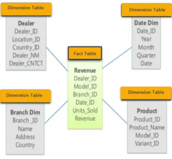
Star Schema A model is called a star schema when the center of the star
is formed by a fact table connected to various dimension tables as shown in figure 1.
Along with the measures, fact tables also contain foreign keys that relate to the dimension tables’ primary keys, thus, allowing to access the fact table through the dimensions joined to it. By concatenating all the foreign keys, the primary key for the fact table is created, known also as composite key. Dimensions are in a similar way composed of primary keys and attributes which play a vital role in business intelligence solutions since they are the source of a report’s labels and constraints. They are what makes a business intelligence system understandable and usable. (Larson, 2008)
Figure 1: Star schema Source: Retrieved from guru99.com
One of the advantages that offers a star schema is it’s simplicity. Business users, even the ones without any technical background find no difficulties at un-derstanding and recognizing the business process that is being modeled through the star schema. Thanks to the reduced number of tables and meaningful busi-ness description, users are less prone to make mistakes while navigating the model. In addition to the usability easiness and thanks to its simplicity, the star schema also offers performance benefits. Due to the low number of joins that characterizes the model, it offers high performing queries.(Kimball & Ross, 2013)
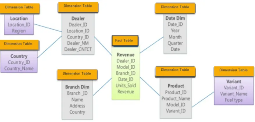
Snowflake schema Another layout that stores dimensional and fact tables
is called a snowflake schema. In a snowflake schema each level of hierarchy is represented by a separate dimension and thus resulting in a normalized data structure. The liaison between dimension tables which resembles the convoluted patters of a snowflake are the inspiration of the model’s name. The figure below is of a snowflake schema.
Figure 2: Snowflake schema Source: Retrieved from guru99.com
Galaxy schema A galaxy schema is one that contains two fact tables
sharing dimension tables. A galaxy schema also know as a fact constellation schema can be constructed through splitting a star schema into multiple star schemes where the fact tables are aggregated on different levels of the dimension hierarchies.
Figure 3: Galaxy schema Source: Retrieved from guru99.com
In a galaxy schema, each level of the hierarchy is built into a separate dimen-sion. The dimension tables are connected to the fact tables which are aggregated on the same level, thereby allowing better understanding. On the other hand, designing a galaxy schema can be very complicated due to the different levels of aggregations.
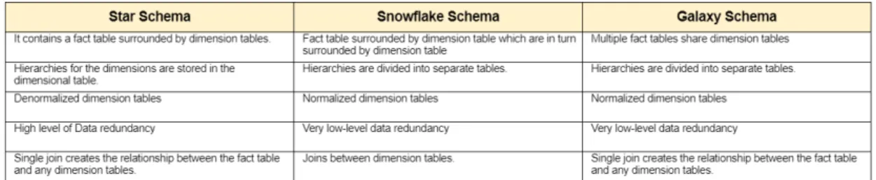
The following table summarizes the differences between star, snowflake and galaxy schema.
Figure 4: Comparison table of different data warehouse schemas
2.4
Data mart
There are three types of data warehouses, in this report, the focus will be on one type (data mart) and its features.
2.4.1 Data mart types
While data warehouses tend to be large repositories containing all the historical data of an organization, a data mart on the other hand, is usually smaller than a DW, focusing mainly on a single subject area such as marketing, sales, etc. According to the data source, three types of data marts can be distinguished.
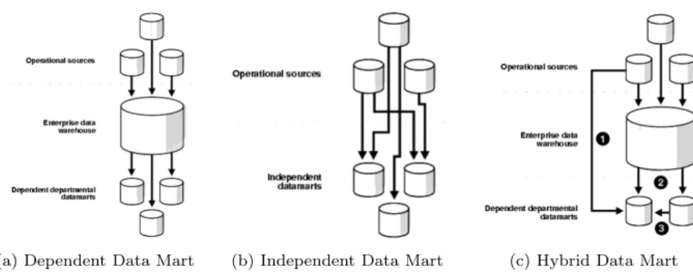
• Dependent data marts are a subset of the DW that has already been created beforehand, they are easier to build since they draw data which has been already cleaned and formatted, providing quality data at the end.
• Independent data marts are standalone systems, built from drawing data directly from various sources. The number of sources is expected to be less than a DW since data marts focus on a single area. However, all the process of extracting, loading and transforming data needs to be dealt with when building an independent data mart.
• Hybrid data marts mix data coming from DW and other sources.
2.4.2 Data mart structure
The different elements that constitute a data mart can be divided into four categories; measures, dimensions, attributes and hierarchies.
(a) Dependent Data Mart (b) Independent Data Mart (c) Hybrid Data Mart
Figure 5: Data mart types Source: Retrieved from docs.oracle.com
• Measures: they are the building blocks for business intelligence solutions. They are usually numeric and additive quantities providing information about some aspects of a company’s performance and are used to support decision making. Number of sales units are an example of a measurement. They are also know as facts and are stored in fact tables. (Larson, 2008) • Dimensions: they are the textual context associated to a measurement. Measures are important for decision making however one single aggregate that represents the total sales for all products for different stores for the entire lifetime of a company’s isn’t usually the used measure to support decision makers. Rather than a single aggregate measure, decisions makers would like to slice and dice the data, dimensions allow the slicing and dicing of data. (Larson, 2008)
• Attributes: they are used to store additional information about dimension members. Records in a data mart can be viewed or filtered through differ-ent attributes of a dimension depending on the user’s requiremdiffer-ent.(Larson, 2008)
• Hierarchies: they are the structure that holds dimensions with two or more levels. For instance a product hierarchy contains a product cate-gory, subcategory and the lowest level of the hierarchy, the product itself. Hierarchies allow users to navigate different levels of granularity of the same measure in a data mart.(Larson, 2008)
When dimension and fact tables are brought together, they form a model referred to as a dimensional model. According to the disposition of fact and dimension tables, different types of dimensional models can be distinguished.
3
Elaborated work
3.1
Halys Digital & Ipsen
This internship was carried out within Halys Digital. Halys Digital is consul-tancy company that has been founded by the president Sylvain Le Moel in 2015 who has brought to the company an expertise build for more than 20 years in the field of business intelligence and precisely in developing solutions with MicroStrategy.
Halys Digital is a human enterprise organization counting around 25 em-ployees that support various clients in their digital transformation by providing services in these different fields going from Mobile Application or Business Intel-ligence to Business Process Management (BPM) and ETL. To assist the clients, a range of tools are used, for instance BPM solutions are developed through Appian whereas MicroStrategy is utilized to develop business intelligence solu-tions.
One of Halys Digital’s clients is Ipsen. A french pharmaceutical company founded in 1929 and reaching to 5700 employees world wide. Since its creation, Halys Digital has been supporting the development of ETL and BI solutions for Ipsen using SAP BODS and MicroStrategy respectively.
Today, Ipsen has decided for purely financial reasons to stop working with MicroStrategy and switch to using Power BI in the creation of their reports and BI solutions. Therefore, Halys Digital has now to create an expertise in developing solution with Power BI, a tool that hasn’t been used at all in Halys Digital. In this context, comes this internship as a first step to start using Power BI within the company and establishing a know-how around this tool.
3.2
Internship goals
The principal goal of this internship can be considered a general one that consists at building a know-how and expertise when working with Power BI, the new BI tool that will be utilized within Halys Digital when supporting their client Ipsen at developing BI solutions.
On a practical side and in order to build this knowledge, an application needs to be developed with Power BI. One of the application used by Ipsen and named MoBI-DIC was chosen for this purpose. The choice of the application to redevelop was mainly based on the frequency of use, its cruciality to improve decision making in the company and that it contained a security level applied to the data. Due to all these factors, the application MoBI-DIC was chosen to be reconstructed with Power BI.
Keeping in mind that this internship purpose is mainly to experiment with Power BI and to test all the possible ways and methods that can be used to re-build MoBI-DIC. In this sens, three possible solutions were identified according to the data connectivity mode and data source type.
1. DirectQuery connected to SQL server database 2. Import mode connected to SQL server database
3. Live connection to SQL Server Analysis Services (SSAS) tabular model
By the end of this internship, a better idea of the challenges that were faced whether when it comes to creating visuals or modeling the data should be provided along with the solutions that were used to overcome them.
3.3
MoBI-DIC
The application MoBI-DIC was chosen as the first application to migrate from Microstrategy to Power BI. It is a sales application developed for French market only due to the different legislation that governs the french pharmaceutical industry when it comes to data security. It is used by over 250 users which are mainly sales representatives, regional managers and operational users.
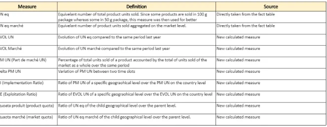
MoBI-DIC provides sales data and measures aggregated first on the market and product level and also on various geographic levels; country, region, sector and UGA. The table below lists the different measures that are used within MoBI-DIC.
Figure 6: Measures used in MoBI-DIC
One specific characteristic of MoBI-DIC is the security that is applied to the data. A user is only allowed to see the sectors that are assigned to him/her but he/she also needs to be able to view the data of the parent region to the sectors along with the country level. A person who has access to a region will automatically be able to view all the data of the sectors belonging to that region.
3.4
Data source
For development purposes, only a snapshot of the data warehouse was provided. The MS SQL server database (DB) contains seven dimension tables and a fact table:
• TD MONTH: Date dimension containing a primary key MONTH ID in the format YYYYMM.
• TD ORIGIN: Origin dimension table; the origian of the purchase, whether the product is prescribed or is bought freely from a drugstore.
• TD PERIOD: Period dimension table; contains various predefined periods such as month, rolling 4 which is 4 months from the current month, etc. • TD UGA: UGA dimension table; contains all information about the lowest
level of granularity of the geographical level.
• TD SECTOR: Sector dimension table; same as TD UGA but on the sector level which is the parent level of UGA.
• TD REGION: Region dimension table; same as TD UGA and TD Sector but on the region level which is the parent level of sectors.
• TD PRODUCT: Product dimension table; contains all the information about various products.
• Fact SOG : fact table on the lowest granularity level which is the UGA and the product level.
3.5
Data schema
When looking at the nature of the measures that need to be provided through MoBI-DIC, one can notice that the information needed to be always provided is on different geographic levels for market level and for product level. The idea is then to build fact tables that are explicitly assigned to dimension tables at different granularity levels. Thus, resulting in a fact constellation schema also known as a galaxy schema.
Views were created in order to act as aggregated fact tables. At the end, five new fact tables were created:
• FACT SOG CTY : Fact table on country level
• FACT SOG MKT CTY: Fact table on country and market level • FACT SOG REG : Fact table on region level
• FACT SOG MKT REG: Fact table on region and market level • FACT SOG SCT : Fact table on sector level
• FACT SOG MKT SCT: Fact table on sector and market level • FACT SOG MKT UGA: Fact table on UGA and market level
In order to make the galaxy schema ready to be used by Power BI, few things needed to be addressed first:
• Setting relationships between fact tables and dimension tables: constraints need to be added to the fact tables, foreign keys were set in order to allow data integrity and for the data or measures to be sliced and diced through dimension tables.
• Datetime fields needed to be added to fact tables: the original fact tables provided did contain a date key of type integer that connected the fact
table to the dimension table. However, in order to use time intelligence functions in later stages to answer the users’ needs of business intelligence analysis and enabling data manipulation using time periods, a new column of datetime type needed to be added to the fact tables.
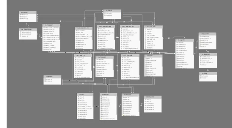
MoBI-DIC schema is presented below
3.6
Developed solutions
3.6.1 DirectQuery mode
DirectQuery is a data connection mode in Power BI which does not load data into Power BI model. With this mode, data will reside in the data source. When connecting to the data source, the schema and the model’s shape will be copied, the actual semantic model definition will be inside power BI desktop but the data itself will stay in the data source. Each time the user interacts with a visualization, a query will be issued directly to data source.
In the following section, an explanation the different pages/tabs constituting the report and how were they build, the difficulties and challenges faced and how they were overcome will be given:
3.6.2 Report composition
Global Analysis - Analyse Globale in this page, four tables are presented,
each on a different geographical level. Each table provides information about the number of products sold along with other calculations and created measures. Each table contains the following data on different aggregation levels (Country, Region, Sector and UGA):
• UN eq: number of equivalent products sold. The use of equivalent is due to the fact that some medications were prescribed in 50g and some in 100g, therefore and in order for data to be compared easily, the equivalent number was adopted. The UN eq is taken directly from the fact tables and used within the table visual.
• UN eq march´e: number of equivalent products sold on the market level.
Similar to product level, the use of equivalent number of products sold is
for comparison reasons. Like UN eq; Un eq march´e is taken directly from
the fact tables and used within the table visual.
• EVOL UN: is a measure that presents the evolution of UN eq compared to same period last year. Using DAX, a first measure that returned the UN eq of same period last year was created. It was then used again inside the measure EVOL UN. Conditional formatting was applied to EVOL UN, the font color of negative numbers was red in contrast to green for positive values. The conditional formatting option of front color was used in order to reach these results.
Figure 8: DAX formula for intermediate stage of EVOL UN
Figure 9: DAX formula for EVOL UN
• EVOL March´e: is a measure that displays the evolution on UN eq march´e.
Similar to EVOL UN, two measures using Data Analysis Expressions (DAX) were created to achieve the desired output.
• PM UN: is a measure that returns the percentage of product from the whole market level. A simple division formula was employed to calculate PM UN
• Delta PM UN: is a measure that subtracts the current PM UN from the same period last year PM UN. Through DAX and the time intelligence functions, the measure Delta PM UN was created.
• Delta PM UN (pts): The user required that for the measurement Delta PM, the unit should be a text string pts. Therefore, using the below formula, unwanted behaviour was checked and returned a blank in case the measure itself is blank. In order to achieve the desired formatting outcome that consisted of having negative values in red and positive values in green, the conditional color formatting rule was used based on Delta PM UN and not this measure itself because it contained a text string.
Figure 10: DAX formula for Delta PM (pts)
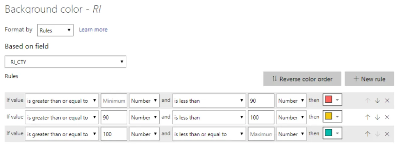
• RI: is a measure that calculates the implementation ratio of a market of each geographical level compared to the country level. For RI, the conditional formatting consisted at coloring the background of cell with red, orange or green according to a specific rule as shown below.
Figure 11: Background formatting rule for RI
• RE: is a measure that divides the EVOL UN of each geographical level by the EVOL UN of the country level. The same conditional formatting of background cell color of RI was applied to RE.
• Quota produit: is a measure of the product quota of the current geograph-ical level compared to the parent level.
• Quota march´e: is a measure of the market quota of the current geograph-ical level compared to the parent level.
A few challenges were faced when building this page of the pbix file. The first one is that this report is used only in France, therefore, users required that the thousand separators should be a space and not a comma which was the thousand separator offered in Power BI. To do so, the regional setting on the machine needed to change first. French(France) as the format of numbers was selected. Afterwards, change the regional settings of Power BI to use French(France) instead of the default value. Changing the regional settings on Power BI alone will not result in any changes in the interpretation of numbers or dates, etc. It is important to change the regional settings of the machine.
The second challenge is related to the measures Quota produit and Quota
march´e. The DAX expression of Quota produit is presented in figure 13. One of
the requirements set by the user is the activation of multi-selection for a number of slicers. One of these slicers is the region slicer. When the user selects only one region and using the following DAX formula, the calculated values for Quota
produit and Quota march´e on the sectors level are then correct as shown in the
figure 14.
Figure 13: Dax formula for Quota Produit
Figure 14: Returned values when selecting only one region
However, when the user selects multiple regions, then the returned values
for Quota produit and Quota march´e are incorrect. As observed in the below
figure, instead of having 6.3% and 10.6% for Quota produit and Quota march´e
respectively, the calculated values are 1.9% and 4.8%. These values are wrong because when using the above mentioned DAX formula and since there is no possibility to set parent-child relationships in tabular models. The calculation of the measures will consider as parents all the selected regions and will not be able to determine to which region each sector belongs to. For instance, when using multi-selection scenario and taking sector A001 as an example, the wanted measurement will be divided by the total values of both regions A and B which are selected in the multi-selector slicer and not just region A.
Figure 15: Returned wrong values when selecting multiple regions At the beginning of the project, the provided solution to overcome this issue was to add to each table the parent geographical attribute. At the end, all tables will have the correct measures but will also contain the parent and child level of various geographical levels, not a very visual friendly solution since there is a lot of redundancy. Moving forward in the project and developing further DAX skills, another solution was adopted that consisted at re-writing the DAX formula as shown in figure 16 to then being able to remove the added parent column of the geographical levels to all tables.
Figure 16: Updated DAX formula for Quota Produit
Mapping Region , Mapping Sector and Mapping UGA these are three
different pages of the report. Each page contains a list of slicers that filter a scatter plot. RI and RE are the two measures that are presented on the axes whereas the size of the bubbles represents the number of sold products.
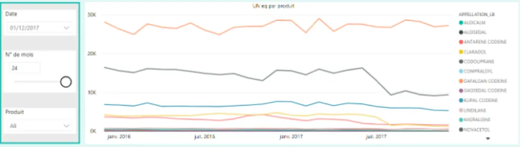
Evolution of PM and UN eq the purpose of this page is to provide two
graphs that display the evolution of UN eq and PM for the last 24 months. The outcome is to display the 24 months of data for PM and UN eq based on one date selection. Usually, when selecting a date in Power BI, it will filter down the other visuals on the page and for one date, only one data point for each product will be displayed on the graph and not a continuous line.
Figure 17: Wrong behaviour for evolution chart of UN eq
The idea is then to disconnect the date table used in the slicer from the graph to be able to show previous months of data. In other words, the date table that will be used in the slicer should not be the same date table that is connected to the fact table. Therefore, a new date table was created using DAX, the distinct function was called to return a one-column table of distinct values of a specified column, in this case the specified column was the date attribute of the date table. The next step consisted at making sure that the new table isn’t connected to any of the fact tables. Afterwards, measures were needed to be created in order to be able to return the values for the 24 rolling months.
The idea behind these measures is to filter down the graphs or visualizations for the last 24 months. To create these measurements, various DAX functions were used. For instance, to harness the date that is selected on the slicer, the MAX function was used. This value was then stored into a variable using the VAR function. After harnessing the selected date from the slicer, then previous 24 months was then calculated. Using time intelligence function DATEADD, a table that contains date columns shifted backward in time by a specified
number of intervals, in this case by 24 months. Actually, one enhancement that was suggested between the Microstrategy solution and the Power BI solution is that instead of using a fixed date range to look backward into the data, the user can actually specify the time range the he/she would like to analyse. A parameter was created for this purpose and was then passed as an argument to the DATEADD function. At the end two variables are created, one containing the current date which is marked on the slicer and the other containing the previous date that is the backward of the current date by the number of intervals set by the user as showen in the below picture.
Figure 18: DAX formula for the evolution of UN eq
The last step in the DAX formula consisted at calculating the number of sold products but only for the desired period, in other terms filtering the fact table using the current date and the previous date stored in the new variables. The returned variable will contain the results of the CALCULATE function. The output is shown in the figure below.
Figure 19: Correct behaviour for evolution chart of UN eq
Comparaison RI/RE is the last page of the report. In this page, a matrix
graph was used to display RI and RE for different products over all periods. In case of RI and RE were over or below a certain limit set by the client, the user wanted to replace these values by a text string. This goal was again achieved using DAX. Taking as an example the RE measure, the SWITCH function took as an argument TRUE function to evaluate the rest of the arguments. If the scalar value returned from the comparison of RE with the limits set is different from the evaluation expression which is TRUE function in this case, then display
the chosen text string instead of the original value else return the measurement value.
Figure 20: DAX formula to change RE
Tooltips one of the common features that was utilized by users when working
with reports developed via MicrtoStrategy was information windows. When a user clicks on an object such as a cell in a table, an information window pops up over the element to display further information. After viewing the information, the user then can close the information window by pressing the ”X” on the top right corner.
The exact behaviour couldn’t be replicated with Power BI, nonetheless, a similar one was used. Instead of having pop-up windows when clicking over an object, the user will have a pop-up window when hovering over an object. In this case, tooltips were used when hovering over the country, region or sector name in the first page of the report. The additional information that was presented through the tooltips was the mapping of RI/RE. When a user will hover over a location, he/she will be able to analyse the RE/RI for the geographical level just below.
The picture below shows the tooltip that is produced when hovering over Region A, the tooltip will display the scatter plot of RI/RE of all sectors be-longing to that region while applying the context from the slicers in that report page.
Figure 21: Tooltip when hovering over Region A
To create a tolltip, first a new report page needed to be created where in the page size setting of the format pane, the developer can choose a page size from the drop down list. Instead of using the predefined type of tooltip, the choice was to use a custom page and then adopt its size to the specific needs since the predefined tooltip was too small to visualize the data neatly.
Figure 22: Choosing page size type
After creating the tooltip as a custom page, the second step is to place the visuals. It is recommended to set the Page View on the View tab of Power
BI to Actual Size instead of Fit To Page before building the graphs, so that when building the graph, it will not be smaller or bigger than the actual space. Furthermore, it is important to turn on Keep all filters so that the context of the original page will be applied to the tooltip. Through the below graph, it is possible to observe that the context from the first page will be applied to this tooltip.
Figure 23: Tooltip settings
The last step consists at configuring the tooltip and apply it to the visual that it is supposed to use it. This is achieved by selecting the target chart and under the Format pane, turn on the tooltip and selecting the name of the desired tooltip.
Figure 24: Applying the tooltip page
Drillthrough is used to further enhance the reporting experience. It is used
to navigate between different report pages while focusing on a data point. The Evolution PM & UN EQ was set as target page to drillthrough from the first
page Analyse Globale. The entities that the drillthrough was provided for are region and sector. In this case, it was important not to pass the filters to the drillthourgh window since the purpose is to use the drillthrough page to compare the same measure over several products, however, if all filters from the source page will be kept then the graph will be filtered to single product which goes counter to the wanted behaviour.
Figure 25: Drillthrough from the region entity
Nonetheless, except the product slicer, all the other filters should be passed on to the drillthough page. To do so, instead of using keep all filters, Power BI offers the possibility to sync slicers individually across various report pages by choosing a slicer and choosing to either sync it with other pages, makes it visible in the other page or both options at the same time.
Figure 26: Sync slicers
Row Level Security (RLS); in MoBI-DIC, the RLS should be defined in a
way that when a user has access to a region, he/she will be able to see the data of the above level which is the country level, France and all the sectors belonging to that region. On the other hand, when a user has access to a specific sector, he/she is supposed to able to view all the data of the above levels, which are the region that the sector belongs to and the country level.
Power BI offers the possibility to define roles to restrict data access for users. It was clear that static RLS can’t be adopted within MoBI-DIC because it can’t be maintained due to the huge number of users which implicate that for each user a different role should be created. It is hard to imagine that no mistakes will be made when maintaining couple of hundred roles and needing to change the DAX expressions on different tables. Thus, RLS needed to be dynamic and based on the users’ login, the data will be filtered automatically.
Dynamic RLS is complex and highly dependant on the data model. Dynamic RLS means that according to the user who will log on, tables will be filtered accordingly. Hence, a new table that contained the user and the region id and sector id assigned to them were added to the schema. The below picture shows that there are two active, bidirectional relationships between the TD SECU table and TD REGION and TD SECU and TD SECTOR. In order to apply security, these two relationships needed to be set to active so the fact tables can be filtered at the end. However, in doing so, the relationship between the TD SECTOR and TD REGION needed to be changed to inactive, meaning that the TD REGION will not be filtering TD SECTOR and that DAX formulas
need to be re-written to provide the correct results. At the end, it resulted in more complicated DAX formulas.
Figure 27: First security schema proposed
With the objective to not change further the DAX formulas, another solution was provided. Instead of adding just one table that will filter both the region and the sector table at the same time, two tables were added to the current model. One table that contained the users along with the regions id attributed to them and another one with users and the sectors id attributed to them. The resulted schema can be viewed in the figure below.
Figure 28: Kept security schema
After updating the schema, it is now time to move on the DAX formula but before to do so, one thing needed to be fixed first. In fact, DirectQuery mode presents some limitations, one of them that not all functions are supported when implementing RLS. Hence, the security tables were switched to import mode in lieu of DirectQuery mode. Afterwards, the following two DAX expressions were added to the correspondent tables
(a) DAX expession of RLS on region level .
(b) DAX expession of RLS on sector level
Figure 29: Row Level Security implementation
The DAX formulas for implementing RLS on regional level can be explained in the following way:
1. Filter the TD SECU REGION table where the user id is equal to the fetched user name using the DAX formula USERPRINCIPALNAME() 2. Select the column named ”Region ID” which is newly created in an
in-memory table and that contains the REGION ID from the filtered table in the previous step
3. Get the distinct output
Same logic is applied to TD SECU SECTOR.
3.6.3 Import Mode
Import mode is a different type of connection to the data source. In this type of connection, all the data will be imported into memory and brought locally to the machine that hosts the Power BI report. When using Power BI report locally, the data will then reside in Power BI desktop and once it is published into Power BI web then the data will reside in the Microsoft data center.
In order to get data up to date, it is either possible to make on-demand refresh or scheduled refresh. Usually when developing professional projects that are used across an organization, it is more common to set a scheduled refresh of the data.
The development of the same application that is MoBI-DIC using import mode didn’t need to start from scratch. In fact, Power BI offers the possibility to switch from direct mode to import mode easily, nonetheless this switching from direct mode to import is irreversible and should be well studied before it is acted on.
The following figure presents the steps taken to switch to import mode. First step is to access the Edit Queries editor and then to select a random table. In the Applied Steps window, the first step named Source needs to be selected. A message with the possibility to switch all tables to import mode will appear. When approving the switch, Power BI will copy all the data from the source to within Power BI desktop. The import mode version of the application was then created and no further steps needed to be taken.
Figure 30: Steps to switch to import mode
The scheduling of data refresh is done after publishing the report into Power BI services. The data in MoBI-DIC should be refreshed monthly, however, the maximum refresh frequency provided in Power BI is a weekly one, hence it was used within this application even though it is not the required one. In fact the most challenging step in configuring the data refresh is actually setting up the connection between Power BI and data source.
3.6.4 Live Connection Mode
Live connection is a connection mode specific to analysis services only. When connecting live to a data source, the actual semantic model and structure will still reside inside SQL Server Analysis Services (SSAS). When using the live connection, it is either possible to connect to a multidimensional model or tab-ular model. However, since the start of the project, it was made clear by the client that due to strategic reasons, he had no interest in working with multi-dimensional models. Therefore, the only solution that will be developed with SSAS is the tabular solution.
The first step is to install a tabular instance on SSAS so that the solu-tion can be deployed on. When installing the SQL server analysis services and during configuration phase, the tabular mode should be selected to insure the installation of a tabular instance of SSAS.
Figure 31: Server configuration; tabular mode
Building a tabular model in SSAS Now that the server is installed, it
is time to start building the model. The next step is to create an analysis services tabular project within Visual Studio which is an environment used to create business intelligence solutions. This project will be deployed on the SSAS tabular instance installed on the server and will result in the creation of an in-memory database that will be later connected to Power BI using the live connection mode.
The logic in creating a tabular solution is similar to using other business intelligence tools, meaning that the first step will consist at selecting the data source and then choosing all the tables that should be loaded into the model. The underlying relationships that are defined in the data source will also be im-ported to the current model. The tabular model explorer allows the navigation of the model using different objects such as data source, tables, relationships and measures as shown in the figure below.
Figure 32: Tabular model explorer
The developer experience between Power BI and Visual Studio is quite dif-ferent when developing a business intelligence solution. For instance, in Visual Studio, DAX measures can be created using the measure grid shown for each table in the Data View.
Figure 33: Tabular model measures definition
Once all the measures and security roles are created, the solution can be deployed. However, the deployment configuration should be set in place before hand. Two things are important to specify, the first one is the name of the tabular instance of the SQL Analysis Services that the solution will be deployed on and the second one is the database name of the Analysis Services database in which the model objects will be instantiated upon deployment. This is the database that will be later on connected to Power BI in order to create the desired reports and visuals. It is important to note that if the name of the model is changed after deployment then the instance of Analysis Services where the solutions were deployed will present separate databases.
Figure 34: Tabular model deployment configuration
When connecting to SQL Server Management Studio (SSMS) and to the Analysis Services tabular instance, the deployed database on this instance can be seen and browsed via DAX when desired.
The final step is to connect Power BI to the tabular instance of Analysis Services and to create the desired visualizations. No intelligence is built within Power BI, everything needs to be defined within the model in Visual Studio. It is important to emphasize that what is selected in Power BI is the the entire model and not specific tables that constitute it. The model will includes dif-ferent tables, their relationships and the calculations that will be connected to Power BI. If some tables shouldn’t be presented to the final user then there is a possibility to hide them.
The entire solution for live connection mode was developed from the begin-ning. A future improvement can be to find a solution that can switch between DirectQuery or import mode to live connection without having to restart ev-erything from scratch.
3.7
Comparison of different solutions
A comparison of the different solutions is vital in order to be able to provide guidance and proper recommendations to the client. Each of these solutions that mainly differ in the connection type to the data source offer certain advantages and disadvantages. A deeper look into this subject will be made in this section. Starting with DirectQuery connection mode. As stated before, in this type of connection, the data will reside in the data source and for each visualization, a query will be sent to the data source to get the required data. When the me-chanics behind DirectQuery mode are understood, the first question that will be asked will relate to the performance of this connection. This is a very important question because one of the major drawbacks of DirectQuery connection is the performance. It was easily noticeable that even with the current relatively small data set provided for the development of the application, the visualization in DirectQuery mode took longer to show up or to refresh.
Moreover, depending on the data source DirectQuery mode only supports a limited number of transformations. For instance, when connecting to SAP Business Warehouse, no transformations are allowed. It is then better advised to use a different ETL tool than Power BI itself when using DirectQuery mode. This mode also sets some limits on modeling and DAX. In fact, calculated tables can’t be created since they are in-memory tables and in-memory tables can’t exist in DirectQuery mode. This was one of the limits faced when implementing security for this application, since the logic used required the creation of an in-memory table, an error message appeared stating that this can’t be done which resulted in finding a workaround around this issue. Furthermore, not all time intelligence capabilities are available in DirectQuery whereas time intelligence functions are a powerful feature of Power BI.
report is used with DirectQuery, a query is sent to the data source resulting in the use of current data in all cases. Another advantage that DirectQuery mode offers is the ability to use massive amounts of data. Since there is no in-memory data stored in Power BI, the only size limit applied to the data is in the data source itself, however, it is important not to forget the effect that this will have on the performance of the report.
To summarize, the following points present the advantages and disadvan-tages of DirectQuery connection mode,
• Advantages
– No data set size limitation; size limitation only for the data source itself
– No data refresh required • Disadvantages
– Limited Power Query transformations – Limited use of DAX and Modeling – Lower performance
Moving to Import Mode connection type. In this connection mode, the data is loaded in memory of the machine that hosts Power BI either on desktop or in the cloud. In this case, it is clear that the performance question will not be raised that much since the data is local and the response time will be super-fast. However, the question that will be raised will be regarding the size of the data and if there’s a limitation on it. Indeed, Power BI limits the entire storage to 10GB with the possibility to upload 1GB of data at a time. This should be an important point to take under consideration when deciding to work or not with import mode. Furthermore, data refresh should be the next question raised with this method. If the requirement of the different stakeholders to have data without delay then import mode can’t be a valid option. In the context of this application, data is monthly refreshed so there is no real constraint regarding this criteria except the fact that establishing the connectivity and configuring the gateway between the data source and Power BI is by far the most challenging task in configuring data refresh.
On the other side, when developing an application while utilising import mode, a full advantage of DAX and Power Query will be taken. These compo-nents of Power BI are the tools that make Power BI an analytical tool and not just a visualization tool. The benefits and limits of a solution developed using import mode are the following,
– High performance
– Full use use DAX and Power Query • Disadvantages
– Requirement to schedule refresh – Data size limit; 1GB per model
Finally, the Live Connection mode. Same as DirectQuery connection mode, for each visualization a query is sent back to the data source but in this case the data source will be an analysis services source running on a analytical engine and consequently the response will be faster. Still not as fast as the import mode but faster than the DirectQuery mode. In this mode, Power BI could be considered merely as a visualization tool, no access to Query Editor, data tab or relationship tab is given. Except for one case, when connecting to SSAS tabular model, there is the possibility to create report level measures that are specific to the report they are created in, thereby leveraging on DAX capabilities. Nonetheless, live connection offers one important advantage that the other two solutions don’t offer, that is a centralized model. At the same time, this mode provides the benefits from two worlds: no data size limits because data is not stored in-memory and the analytical strength when developing tabular models using DAX. To conclude, the list of advantages and disadvantages of live connection mode are presented below,
• Advantages
– Fast performance – Centralized model
– Unlimited DAX within SSAS tabular • Disadvantages
– No Power Query transformations – No access to the schema
After establishing a comparison between the different solutions and under-standing the advantages and disadvantages presented by each one of them. A set of criteria that are considered critical in order to evaluate the developed so-lutions and help in choosing which solution to work with was established. The solutions were then assessed over these criteria. The summary of the evaluation is presented in the table below
Figure 36: Solutions evaluation
4
Conclusion
In a time when the final client is migrating from one business intelligence tool that is Microstrategy to another business intelligence tool that is Power BI. This internship comes in this context to try to explore what can be entirely reproduced with Power BI, what should be changed and what are the key points to consider when making this transfer.
To reach this objective, the following steps needed to be take:
• Identify the different solutions that can be developed with Power BI • Determine and apply the needed changes on the provided data so that it
can be utilized in Power BI
• Build the identified solutions starting from modeling, to calculations’ def-inition and to finally visualizations’ construction.
Through the identification of different connection modes that Power BI of-fers, three different solutions were identified. Afterwards, changes needed to be made to the provided data. The changes mainly consisted of adding constraints between dimension and fact tables and altering fact tables to contain column of datetime type so that time intelligence functions can be used in later stage.
A galaxy schema also known as fact constellation schema was chosen to model the data. In fact, the data needed to be on the lowest granularity level and on the market level for each different geographical level. To be able to visualize this data, it was required that the model had fact tables aggregated on these different levels and connected to dimension tables that are on the same granularity levels. At the end, a schema with multiple fact tables where some of them shared the same dimension tables was created.
Once the model is set, the next step consisted of adding the needed calcu-lations. For import mode and DirectQuery mode, DAX was used within Power BI desktop to create the required measures. When it came to live connection mode, all the intelligence was built inside of Analysis Services.
When comparing the different solutions, import mode and live connection showed the best results when considering the performance factor but when con-sidering the data size, import mode wasn’t a good choice. Therefore, in this specific application, it is better to use live connection mode for the development of this solution.
It is important to consider some key points as general guidelines when devel-oping BI solutions, however, in most of the cases, everything is context related to the application that is developed at the moment. This time, using a live connection to SSAS tabular is the right solution but this shouldn’t be the case for every project in the future. It is crucial to consider the context of each project, the different stakeholders, the story that will be told through the data. All these different factors should be taken under consideration so that the de-veloped solution will be adapted by the user, resulting in the creation of added value to the company.
5
Limitations and recommendations for future
works
Acknowledging the limitations of the developed solution is crucial for the im-provement of future works. In fact, during the development of this solution, the main limitations that were faced were mainly solved using DAX. In fact, is it important to learn how to write smart pieces of DAX code because it can actually improve the performance of the reports. DAX can be seen as a way to unleash more capabilities of Power BI and skills related to DAX should be further developed so that the most performing Power BI reports can be offered to the final users.
Another recommendation is to use Power BI performance analyzer feature. By examining report elements with the performance analyzer, the developer will have the possibility to get information about the time taken by each visual to query the data and to render the results. Consequently allowing the developer to dig deeper into these details and look for ways to improve the report’s per-formance whether by writing more optimized DAX expressions or choosing the appropriate visual to visualize the data.
References
Devens, R. M. (1868). Cyclopaedia of commercial and business anecdotes. D. Appleton.
Heinze, J. (2014). History of business intelligence. Retrieved 20-10-2019, from https://www.betterbuys.com/bi/history-of-business-intelligence Inmon, W. H. (2005). Building the data warehouse. John Wiley & Sons. Kimball, R., & Ross, M. (2013). The data warehouse toolkit: The definitive
guide to dimensional modeling. John Wiley & Sons.
Lago, C. (2018). 150 years of business
intelli-gence: A brief history. Retrieved 18-10-2019, from
https://www.cio.com/article/3290407/history-of-business-intelligence.html
Larson, B. (2008). Delivering business intelligence with microsoft sql server 2008. McGraw-Hill, Inc.
LIMP, P. (2019). Exploring the history of
busi-ness intelligence. Retrieved 20-10-2019, from
https://www.toptal.com/project-managers/it/history-of-business-intelligence
Turban, E., Sharda, R., Aronson, J. E., & King, D. (2008). Business intelligence: A managerial approach. Pearson Prentice Hall Upper Saddle River, NJ.