Modeling the gait using an IMU and FSR

(1)

UNIVERSIDADE DE LISBOA

FACULDADE DE CIÊNCIAS

DEPARTAMENTO DE FISICA

Modeling the gait using an IMU and FSR

Ana Teresa Marinho Viegas

Mestrado Integrado em Engenharia Biomédica e Biofísica

Perfil em Engenharia Clínica e Instrumentação Médica

Dissertação orientada por:

Professor Nuno Matela

Professor Jorge Martins

(2)

(3)

i

Abstract

Drop-foot syndrome is a condition that consists of an inability or difficulty of pulling the foot upwards at the ankle joint. It usually has a neurological cause, where the deep peroneal nerve is not properly activated, meaning that the tibialis anterior, responsible for the dorsiflexion of the foot, is not activated, which functionally results in “drop” of the foot while walking.

To properly diagnose this condition, and other conditions related to the gait, it’s important that a base gait model is established, for comparison.

Throughout the years, different techniques have been used for this purpose, from imaging to using sensors to track the foot while in movement. As technology advances, new, cheaper and more accurate ways to track and model the gait have emerged.

In this project, the tracking of the foot was made by an IMU (Inertial measurement unit), while also using FSR sensors (Force sensitive resistors) to distinguish one step and the next. All the sensors were connected to a microcontroller that rested on the right leg (the leg under analysis) and were itself connected to a computer that recorded the data, via a prebuilt interface. Then, said data, recorded in a .csv file, were analyzed by a MATLAB script, that calculated the position and foot angle.

This method proved effective, but incomplete to create said model. Although still on an initial stage, this method can be improved to be a reliable and useful method to build gait models in the future.

(4)

(5)

iii

Resumo

Síndrome de drop-foot é uma condição que dificulta ou impossibilita a dorsiflexão do pé. Consiste numa deficiência de comunicação com o musculo tibialis anterior, que é feita através do nervo profundo peronial (DPN), que resulta na não ativação do músculo necessário para tal movimento. Esta condição é geralmente fruto de um acidente neurológico ao nível do cérebro (um acidente vascular cerebral, por exemplo) ou algum tipo de lesão no nervo que ativa o músculo, o que resulta numa ativação deficiente do mesmo. Estas lesões e as suas consequências podem ter diversos sintomas e efeitos, que, dependendo da severidade do caso, podem ou não ser parcialmente ou totalmente reversíveis.

Sendo assim, é de extrema importância um correto diagnóstico e escolha de terapia, de forma a proporcionar a pacientes com esta condição o melhor plano de tratamento.

De forma a diagnosticar esta e outras condições, são utilizados modelos da passada, de forma a comparar a passada de um paciente ao esperado e determinar a gravidade da lesão.

Este projeto tem como objetivo testar um novo método de modelar a passada, usando sensores inerciais (IMUs) ligados a um computador através de um microcontrolador.

O dispositivo utilizado consiste num microcontrolador, uma placa lógica e os sensores. O dispositivo é ligado ao computador através de um cabo USB. O microcontrolador já continha todo o código necessário para o seu funcionamento e emparelhava com o interface instalado no computador.

Existem 2 tipos de sensores ligados ao dispositivo: sensores de pressão (FSRs) e sensores inerciais (IMUs). Para este projeto, foram utilizados 5 FSRs e 1 IMU.

Os sensores FSR são posicionados na planta do pé direito, de forma a detetar quando o pé toca no chão. Os dados adquiridos destes sensores irão determinar o início e fim de um passo.

O sensor IMU deteta velocidade angular e aceleração linear. Estes dados irão ser exportados, através de um ficheiro .csv, para um script no MATLAB que aplica os integrais necessários de forma a obter posição e angulo do pé (em relação ao solo).

O sensor obtém estes dados calculando 3 frames principais: o frame intrínseco sensor, que se mantem estático em relação ao sensor e, consequentemente, ao pé, o frame da posição inicial, que é calculado a partir do vetor de gravidade detetado pelo sensor, e o frame do passo, que, como o nome indica, é formado quando é detetado o inicio de um passo. Este último é calculado em relação ao

frame definido pela gravidade. De notar que, enquanto os dois primeiros são calculados

intricadamente no microcontrolador de forma a obter os dados necessários à analise, este último tipo de frame é formado durante os cálculos feitos após o registo dos dados.

Este cálculo, feito num script de MATLAB, é feito usando um modelo já previsto.

O interface é responsável pela recolha e registo dos dados. Quando ativado, ele irá registar os dados num ficheiro .csv, que poderá posteriormente ser lido pelo script MATLAB que irá calcular todos os valores necessários para analise.

Para a analise, foram calculados e usados para comparação a posição do pé no eixo Z (eixo anti paralelo ao vetor gravidade) e o angulo do pé em relação ao solo. Como o sensor IMU apenas deteta aceleração linear e velocidade angular, são necessários integrais para calcular os dados

necessários à analise. Estes cálculos foram feitos num script MATLAB modificados para os fins deste projeto.

(6)

iv Para os cálculos, o script usa a informação do sensor FSR (informação essa é processada anteriormente. O resultado desse processamento é um vetor de zeros de tamanho igual ao dos dados adquiridos, que, quando é detetado um passo, altera o zero correspondente a esse instante para um) para dividir os dados em frames. Por cada novo frame (equivalente a um novo passo), é inicializado um novo integral com novas constantes iniciais. Estas constantes iniciais são assumidas pelo sistema.

Por fim, todos os dados resultantes do cálculo integral são guardados numa matriz, que é utilizada para todas as representações gráficas e alterações necessárias para analise, como por exemplo, o alinhamento dos paços de modo a poder calcular uma curva de valores médios para a posição e angulo do pé ao longo da passada.

Os sujeitos (todos indivíduos com passada saudável) foram instruídos a andar a passo regular, lento e rápido, com o dispositivo instalado na perna direita. De notar que o conceito de “passo

regular”, “lento” e “rápido” foi deixado ao critério de cada sujeito, não tendo existido um compasso para os mesmos seguirem. Consequentemente, pode haver comparação matemática (i.e., comparação e analise matemática, feita de modo quantitativo, dentro de uma função do MATLAB criada com esse propósito) entre ensaios do mesmo sujeito, para a mesma velocidade, mas o mesmo não pode acontecer para diferentes sujeitos, ou diferentes velocidades.

Ao longo do processo, tanto o script como a posição dos sensores foram otimizados de modo a conseguir os resultados mais confiáveis, realistas e reproduzíveis.

Os resultados dos ensaios, após o tratamento de dados, foram comparados com os modelos esperados na literatura.

De um modo geral, os resultados foram razoavelmente semelhantes aos esperados, não se conseguido distinguir nenhuma diferença sistemática entre os valores referentes às diferentes velocidades da passada.

No entanto, dois erros sistemáticos devem ser mencionados. O primeiro corresponde às constantes iniciais referidas acima.

Porque o integral aplicado à aceleração linear é um integral duplo (de forma a obter a

posição), o sistema assume duas constantes como sendo 0: a posição inicial (correspondente á origem do frame criado quando se inicia uma nova passada) e a velocidade linear inicial. No entanto, esta velocidade, na prática, nunca é 0 absoluto. Devido a este facto, existe um declive entre a posição inicial e a final onde os valores das mesmas deveriam ser ambos iguais a zero. Especificamente, no eixo Z (eixo perpendicular ao chão, com direção ascendente).

Após analíse, foi concluído que este erro não tem qualquer padrão, tanto entre sujeitos como quando comparando ensaios do mesmo sujeito.

O segundo erro corresponde a diferença entre as coordenadas do fim de um paço e as do início do próximo, no frame da posição inicial. Este erro deve-se não só, mas também ao método de deteção do passo.

Idealmente, estas coordenadas, no frame da posição inicial, seriam matematicamente iguais (i.e., o instante que finaliza um passo inicia o próximo). No entanto, devido ao método utilizado no projeto (ambos de iniciar um novo integral por passo e da deteção pelo sensor FSR), pelo menos um instante de tempo não irá ser calculado (porque a frequência de aquisição foi de 80Hz, este instante corresponde a 1/80 de segundo). Sendo assim, e porque novas constantes iniciais são calculadas a cada novo passo, existe uma discrepância entre estes dois instantes, em particular no eixo Z.

(7)

v Tal como no erro anterior, não foi encontrado qualquer tipo de padrão, tanto intra-sujeito como inter-sujeito.

Apesar das limitações do método, existe potencial em utilizar este método para modelar a passada com resultados repetíveis e confiáveis. Para melhorar o seu funcionamento, o script onde é calculado os integrais necessita de otimização, e seria necessário um método mais robusto e standard de aplicar o IMU ao pé de futuros sujeitos.

Ainda assim, este provou ser um bom método para criar futuros modelos da passada com o propósito de desenvolver melhores técnicas de diagnóstico.

(8)

(9)

vii

List of figures

Figure 1.1 Lower leg. Adapted from [12]. ...2

Figure 1.2 Gait description. Adapted from [13] ...3

Figure 1.3 Main characteristic of drop-foot syndrome. adapted from [19]. ...4

Figure 1.4 Example of rotation matrix. Adapted from [27] ...8

Figure 1.5 Diagram showing how a new frame and rotation matrix is formed. Adapted from [28]. .... 12

Figure 2.1 Simplified control board architecture, adapted from [10] ... 13

Figure 2.2 Logic board connecting all the components to the interface in the computer. ... 14

Figure 2.3 Diagram of simplified mathematical calculations necessary for position and orientation. .. 17

Figure 2.4 Variables and their respective meanings. Adapted from [27] ... 18

Figure 2.5 calibration graphic. The black line refers to the sections that the script uses to form a calibration matrix (sections where the velocity is close to 0) ... 19

Figure 2.6 Positions of the IMU, in meters, for each step, for the 3 axes. the blue points represent the end of the integral. the red represents the correction. ... 22

Figure 2.7 Positions, in meters, in the 3 axes after removing the correction. ... 22

Figure 2.8 the device strapped to the leg (on the left) and the ideal positioning of the IMU axis (on the right) ... 23

Figure 2.9 Interface used for this project. ... 23

Figure 3.1 linear acceleration and angular velocity of the foot ... 25

Figure 3.2 Raw data of the IMU, converted to standard units and divided per step ... 26

Figure 3.3 Axis and rotation direction. Adapted from [32] ... 26

Figure 3.4 Integrated data, adapted to standard units... 27

Figure 3.5 Z axis positions for each step in one trial, and average of said steps ... 28

Figure 3.6 zoomed aligned z axis positions... 28

Figure 3.7 ankle rotations in the Y axis for each step in one trial, and average of said steps ... 29

Figure 3.8 Average foot angle for different walking paces ... 29

Figure 3.9 average position in the Z axis for different walking paces ... 30

Figure 4.1 FSR detection using the first method ... 33

Figure 4.2 FSR detection using the final method ... 34

Figure 4.3 Ideal Z axis position during the gait. Adapted from [33]. ... 34

Figure 4.4 Position, in the Z axis, of subject 1's foot, while walking at a slow pace ... 35

Figure 4.5 Position, in the Z axis, of subject 1's foot, while walking at a normal pace ... 35

Figure 4.6 Position, in the Z axis, of subject 1's foot, while walking at a fast pace... 36

Figure 4.9 Position, in the Z axis, of subject 2's foot, while walking at a fast pace ... 37

Figure 4.12 Position, in the Z axis, of subject 3's foot, while walking at a fast pace... 39

Figure 4.13 Expected shape of the curve of the foot angle in relation to the floor. Adapted from [34]. ... 40

Figure 4.14 Foot angle of subject 1's foot, while walking at a slow pace ... 40

Figure 4.15 Foot angle of subject 1's foot, while walking at a normal pace ... 41

Figure 4.16 Foot angle of subject 1's foot, while walking at a fast pace ... 41

Figure 4.17 Foot angle of subject 2's foot, while walking at a slow pace ... 42

(12)

x

Figure 4.23 Error within a step for subject 1. ... 45

Figure 4.26 Error between steps, for subject 1. ... 47

Figure 4.27 Error between steps for subject 2. ... 48

(13)

1

1. Introduction

1.1. Motivation

Every year, around 5 million people become disabled due to strokes, as well as 250 thousand due to cerebral palsy and 250 to 500 thousand due to spinal cord injuries. Adding to those numbers, 2 to 3 million people suffer from head traumas [1]–[4].

These injuries can cause malfunctioning of the members, which can imply a struggle to do basic movements, such as grab an object, or walk [3], [5]. Regarding walk related impediments, 76% are what’s called dropfoot syndrome, in which the foot is overly extended [6]. This happens due to a lesion in the deep peroneal nerve (DPN), that innervates the tibialis anterior (TA), the muscle

responsible for the dorsiflexion movement of the foot [7]. These types of injuries can cause spinal and hip lesions in the long run [8].

The motivation for this project is to contribute to the research and development of a model of the lower leg. The project was developed in the Robotics lab of IST, under the guidance of professor Jorge Martins, where other former students and researchers have developed other projects with a similar theme and common ultimate goal, including the main device and software used in this project [9], [10].

1.2. Objective

The device used registers signals from 1 inertial measurement unit (IMUs) and 5 pressure sensors (SP), at a data collecting rate of 80 Hz. The data is obtained through the USB connection. [10] The device allows for a normal use of the leg, within distance of a computer, since it needs to be connected in order to record data. [10]

The goal of this project is to provide a new way of building a gait model that can be reliable and simple to set up.

In the research lab where this project was developed, there have been previous works building and developing the software and hardware, as well as data analysis with the end overall goal of building a reliable gait model for all types of walking (running, up and down stairs, with various slopes, among others).

This project will serve as a proof of concept for future projects that aim to build better and more accurate gait models that can be used to diagnose and manage or even heal any illness or injury talked above.

(14)

2

1.3. Anatomy

1.3.1. Lower limb

Our lower limb can be divided as the leg and the foot. The upper leg (femur) is connected to the hip through a ball-socket joint, while connected to the lower leg (fibula and tibia) through a hinge type joint, at the knee. The lower leg is connected to the foot through a hinge type joint as well, as ti can be seen in the figure below. [11]

Figure 1.1 Lower leg. Adapted from [12].

The muscles controlling the lower leg can be divided into 3 groups: anterior, responsible for the plantar flexion, posterior, responsible for the dorsiflexion, and lateral, which is responsible for eversion/inversion and pronation/supination [4].

In this project, we’re going to focus specifically on the muscle responsible for the dorsiflexion, the tibialis anterior (TA). The TA starts at the distal part of the top of the tibia and covers 2/3 of said bone, attaching itself to the proximal lateral surface of the tibia.

1.3.2. Gait

A full gait cycle is defined as the movement of a chosen lower limb between 2 consecutive heel-strikes. The gait cycle is divided into 2 phases: the swing phase, when the foot doesn’t have contact with the ground, and the stance phase, when the foot is supporting the body.

During the swing phase, the foot will move and adapt to withstand the weight of the body in the next stance phase. During the stance phase, the foot stands stationary, while the ankle rotates, making the body go forward.

(15)

3

Figure 1.2 Gait description. Adapted from [13]

As described in the image above, the majority of a normal gait is single leg support.

For this project, the beginning of a step is defined as the instant where the right foot leaves the ground and ends the instance just before the foot leaves the ground for the next step. It will also only be considered the right leg for measurements.

1.4. Gait problems and solutions

1.1.1. Dropfoot syndrome

Dropfoot syndrome is the common name for a condition that is characterized by faulty or absent dorsiflexion of the foot, meaning that the ankle movement where the foot moves up on that axis is faulty or not possible at all, causing the foot to “drop”, as showed in the image below. This

condition is usually caused by neurological conditions that affect the peroneal, like multiple scoliosis, or accidents, like head trauma, brain or spinal cord injury, or stroke [14]–[16]. To be noted that any other obstruction of the deep peroneal nerve (DPN) can cause dropfoot, such as pressing on the nerve when we cross our legs while sitting. However, that can be resolved by simply changing the habit over time [17]. The first symptom is characterized by slightly dragging the toe on the ground during the swing phase. This is particularly problematic when using stairs or uneven terrain, for example. This forces the individual to adapt their way of walking, which can cause problems to the spine and hips [18].

(16)

4

Figure 1.3 Main characteristic of drop-foot syndrome. adapted from [19].

1.4.1. Uses of gait analysis

Gait analysis is the process of comparing the gait of a subject to the gait modeled by previous studies or papers, and is used mainly on clinical research. This means that, unlike a clinical trial, the goal is not to decide the procedure for the patient, but to study a group of people with a specific characteristic. For example, if a measurement on one patient has many random errors, a conclusion cannot be taken regarding that patient. However, if the same test is performed in many patients, even with many random errors, that data can still be useful and lead to conclusions in research. Usually, it has 4 main objectives [20], [21]:

1. To distinguish Diagnosis between disease entities (diagnosis).

2. To determine severity of disease or injury (i.e. assessment or evaluation) 3. To select among treatment options

4. To predict prognosis and outcomes of intervention

Often, gait analysis is used as a test for patients with neurological conditions the affect motion, such as cerebral palsy or dropfoot syndrome [10], [22].

The third of these might actually be taken as a definition of the word clinical i.e. a clinical test is one conducted in order to select from among different management options for a patient (including the possibility of not intervening) [20].

Despite being around for quite a long time [23], and offering better results than any other method [24]–[26], there’s a very small amount of systems using foot mounted inertial navigation, due to hardware limitations and patent protections, and the complexity of the integration required, making it not very universal. Another problem with the system is that, in a sense, it is virtually blind and requires other tools, such as a GPS, for example, to be precise.

(17)

5

1.5. Physics of the gait and useful mathematical notions

1.5.1. Quaternions

In order to be able to use multiple versions of data at the same time, while keeping them apart (for example, acceleration values for 3 axis), it’s common to present that data in the form of

quaternions to make calculations.

First, it’s necessary to define quaternion.

Given 2 complex numbers A=a+bi and C=c+dj, if we construct a new complex number Q=A+Ci, which would be defined as:

Q=a+bi+cj+dk, (1)

k being ij [27].

We can represent quaternions in different manners, for example:

Q = qw + qxi + qyj + qzk ⇔ Q = qw + qv, (2)

qw is a real number that can represent a quantifiable unit or a scalar, and qv is a vector or a

rotation. None of the variables are in the same scale, though, so, they have to be represented as such [27]. So, we have: Q = [q_qw v] = [ qw qx qy qz ], (3)

This is used to, for example, store any kind of data in a given instant in time.

Operations

Sum operations are trivial.

p ± q = [ pw pv ] ± [qw qv] = [pw ± qw pv ± qv], (4)

The product is slightly more complicated, and not really practical to do by hand.

𝐩 ⊗ 𝐪 = [ p𝑤q𝑤− p𝑥q𝑥− p𝑦p𝑦− p𝑧p𝑧 p𝑤q𝑥+ p𝑥q𝑤+ p𝑦p𝑧+ p𝑧p𝑦 p𝑤q𝑦− p𝑥q𝑧 + p𝑦p𝑤+ p𝑧p𝑥 p𝑤q𝑧+ p𝑥q𝑦− p𝑦p𝑥− p𝑧p𝑤 ] (5)

(18)

6 Another way to describe it would be:

𝐩 ⊗ 𝐪 = [ pwqw− pvTqv

pwqv+ qwpv+ pv× qv] (6)

For pure quaternions, i.e, quaternions whose real part, pw, is zero, the above expression

translates to:

pv⊗ qv= −pvTqv+ pv× qv = [−pvTqv pv× qv] (7)

Note that p ⊗ q is not the same as q ⊗ p. however, (p ⊗ q) ⊗ r = p ⊗ (q ⊗ r). Skew operations:

The notation of this operator is [•]×, and it’s a matrix with the property that it’s transpose

matrix is also its negative, i.e., [a]T× = − [a]×. It can be represented by the below matrix, or a similar

variant. [a]_× ≜ [ 0 −az ay az 0 −ax −ay ax 0 ] (8) Conjugate: q∗_{= q} w− qv= [ qw qv] (9)

Quaternions are often used as orientation or rotation operators. As such, under this conjugate definition, to a rotation operator Q, its conjugate Q* would operate the inverse rotation. For

convenience, rotation quaternions can also be written as such:

q = [cos θ 𝐮 sin θ] (10)

(19)

7 Calculating the quaternion norm:

|q| = √q ⊗ q∗_{= √q}∗_{⊗ q = √q} w 2_{w + q} x 2_{+ q} y 2_{+ q} z 2 ₍₁₁₎

And has the particular property of:

|p ⊗ q| = |p||q| (12)

Exponentials and logarithms

Letting v = u θ, with θ = |v| and u unitary, we group the scalar and vector terms in the series, and recognize in them, respectively, the series of cos θ and sin θ. As we apply this in the following equation, we get this equivalency:

ev_{= e}𝐮θ_{= cos θ + 𝐮 sin θ = [cos θ 𝐮 sin θ]} ₍₁₃₎

To be noted that this is simply an equivalent way to write the same vector, not an equality of vectors.

It is immediate to see that, if |q| = 1,

log q = log(cos θ + 𝐮 sin θ) = log(e𝐮θ_{) = 𝐮 θ = [} 0

𝐮θ] (14)

If we have a rotation vector v = φu, we can define a rotation matrix R as:

(20)

8 Rotations

In the figure below, it’s represented the rotation in ϕ degrees of the vector x around an axis u. we can define x as it’s described by the equations below.

Figure 1.4 Example of rotation matrix. Adapted from [27]

x = x

_∥

+ x

_⊥ (16)

x∥= 𝐮𝐮𝐓x (17)

x⊥= x − 𝐮𝐮𝐓x (18)

Notice that, under the u axis, x’|| = x||, meaning that x|| does not rotate.

x′= x||+ x⊥cos ϕ + (𝐮 × x) sin ϕ (19)

Frames

To exemplify how rotations between frames work, lets create a frame A, defined by:

ex = [ 1 0 0 ] , ey= [ 0 1 0 ] , ez = [ 0 0 1 ] (20)

A vector v, expressed in A, would be:

vA= [vx, vy, vz] = yxex + yyey+ yzez (21)

Now, lets define another frame, frame B, this one defined by the orthogonal unit vectors [rx,ry,rz]. The same way, vB = vxrx + vyry + vzrz.

(21)

9 Writing this relation in matrix form, we have the linear transformation representing the

rotation,

vB = [rx, ry, rz]vA= RvA, (22)

R being [rx , ry , rz].

So, R is the rotation matrix from frame A to frame B.

It’s important to remember that, in order for a vector’s norm to stay the same from one frame to another, the following has to be true.

RRT= RTR = I (23)

It’s important to notice that the product of two rotations matrices is also a rotation matrix.

1.5.2. Trajectory

Rotations as we have seen them so far are instantaneous motions, which means they go from the initial frame to the final frame automatically. In reality, rotations are continuous motions. Meaning an analysis throughout a certain period of time is necessary.

First of all, we notice that it is impossible to continuously escape the unit determinant condition, because this would imply a jump from +1 to −1. Therefore, we only need to investigate the derivatives of the orthogonality condition,

(RṪ_R)_{= R}Ṫ R + RT_{Ṙ = 0,} ₍₂₄₎

which can be rewritten as

RṪ R = −(RṪ R)T_, ₍₂₅₎

which means RṪ R is skew-symmetric. As we have seen before, skew-symmetric matrices can be written as indicated above, in equation (8). We can write RṪ R as:

RṪ R = [ω]

×Ṙ = R[ω]× (26)

ω being a vector of angular velocity.

The solution for this differential equation is [27]:

R(t) = R(0)e[ω]×t_{= R(0)e}[ωt]× ₍₂₇₎

If we write wδt=v, and R(0)=I for that same δt, we have:

(22)

10 Perturbations:

A perturbation Δq can turn the quaternion q into q̃. If q = q(t), then, we can write q̃ as q(t + ∆t). We can relate one another as such:

q̃ = q ⊗ ΔqL, R̃ = RΔRL (29)

Having Δq, the derivative in time of q can be calculated as:

q̇ ≜ lim Δt→0 q(t + Δt) − q(t) Δt = limΔt→0 q ⊗ ΔqL− q Δt (30)

Solving the equation above [27], we get:

q̇ =1

2Ω(ωL)q = 1

2q ⊗ ωL, Ṙ = R[ωL]× (31)

ωL being the angular variation of qL per unit of time Δt.

Time derivatives have the following properties:

(q1⊗ q̇ 2)= q̇1⊗ q2+ q1⊗ q2̇ , (R1̇R2)= R1̇ R2+ R1R2̇ (32) In order to update each rotation in quaternion form, we use the following expression for local rotations:

q(t)̇ =1

2q(t) ⊗ ω(t) (33)

Developing the Taylor series for q(t+Δt) around the time t = tn. Being q(t) = q and q(tn) = qn

and ω(t) = ω and ω(tn) = ωn, the series is:

qn+1 = qn+ qnΔṫ + qnΔẗ 2

2! +

qn⃛Δt3

3! + ⋯, (34)

If we apply this series to the previous expression, we get:

qṅ = 1 2qnωn (35) qn̈ = ( 1 2) 2 qnωn2+ 1 2qnω̇ (36)

(23)

11 q⃛ = (n 1 2) 3 qnωn3+ ( 1 2) 3 qnω̇ωn+ 1 2qωnω̇ (37)

If we assume ω0= 0, meaning ωn is constant between tn and tn+1 , the series can be rewritten as:

qn+1 = qn⊗ (1 + 1 2ωnΔt + 1 2!( 1 2ωnΔt) 2 + 1 3!( 1 2ωnΔt) 3 + 1 4!( 1 2ωnΔt) 4 + ⋯ ) (38)

Which is the Taylor expansion for eωnΔt₂_{. We can use the exponential equation from before}

and write it as:

eωnΔt₂ _{= q{ωΔt} =} [ cos (‖ω‖Δt 2) ( ω ‖ω‖) sin (‖ω‖ Δt 2)] (39) And so, q n+1 ≈ qn ⊗ q{ωn∆t}.

1.5.3. Data acquisition mechanism

Based on all previous notions, we can now start to build the plan for the practical analysis [28].

Typically, in order to obtain navigation data from an inertial sensor such as an IMU, it’s required a zero-velocity inertial navigation system, which consists of the sensors combined with mechanization equations, such as:

[ pk vk qk ] = [ pk−1+ vk−1Δt vk−1+ (qk−1fkqk−1∗ − g)Δt Ω(ωkΔt)qk−1 ] (40) pk = position vector vk = velocity vector fk = specific force

g = [0, 0, g], i.e., gravity vector

ωk = angular velocity vector (given by the IMU)

qk is the rotation matrix, i.e., the quaternion the describes the orientation of the system. (note

that qk−1 fk q *k−1 (i.e., the acceleration estimation given by the IMU) is the rotation of fk by qk, and

(24)

12 During a step, the system is reset when the foot hits the floor, meaning that all calculations regarding velocity and position are taken based on that position. The distance walked

(dead-reckoning), i.e., the distance between the beginning of two steps, as shown in the image below, can be calculated by: [x_χl l] = [ xl−1 χl−1] + [ Rl−1Δpl Δψl ] + wl (41)

Where xl and χ l are the initial position for each step of the system in reference to the navigation frame,

and Rl is defined by the rotation matrix:

Rl= [

cos χl − sin χl 0 sin χl cos χl 0

0 0 1

] (42)

For every step, the initial position xl, which builds the navigation frame l, is updated to xl+1,

which forms a new navigation frame l+1, and all calculations between xl+1 and xl+2, are made based on

the formed l+1 frame. These mechanics are better shown in the image below.

(25)

13

2. Methods

With the goal of measuring and registering the linear acceleration, angular velocity, and heel-strike moment, an IMU and 5 FSRs were used, as described before. However, that information needs to be processed in order to be analyzed properly. This chapter is dedicated to how every process, from device building to the end graphics, was made.

2.1. Equipment description

The device used is divided in 3 sections: the microcontroller, the logic board, and the sensors (1 IMU and 5 FSRs). Despite the fact that it was only used 1 IMU, the system requires 4 to be connected, because of the clock code used to record the data from them. Regarding the FSRs, despite only being necessary one to detect a step, often, the one chosen didn’t detect it properly (because of the foot position, unbalance that resulted in not enough pressure in the sensor, or some sort of unevenness in the terrain), so, regarding that specific take, one of the other 4 FSRs was use instead.

Overall, the data wasn’t too affected by this case to case change. The overall system is organized as showed in the image below.

Figure 2.1 Simplified control board architecture, adapted from [10]

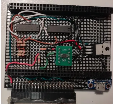
The microcontroller is connected to the sensors and computer by a logic board (seen in figure 2.2, below) that sits over it, connecting to its pins. It works as a communication bridge between all components, and it’s powered by a voltage regulator of 3.3V (the black and silver transistor in the board in figure 2.2), that draws power from the USB (which is 5V). The FSR sensors work as resistors and are connected to AMPOPs (the 2 black bars), which are also connected to a constant resistor (the resistors visible below the AMPOPs, all aligned). This configuration allows the system to calculate the value of the sensor by reading the value of Vk in the OUT pin of the AMPOP.

The IMU sensors are all connected to a Multiplexer (the green square in the board), whose clock is programmed into the microcontroller that registers the data in a cycle, one at a time.

(26)

14 All the sensors are connected to the board via the pins at the bottom of the figure, using the black connector that is visible.

Figure 2.2 Logic board connecting all the components to the interface in the computer.

The microcontroller was a cortex-M4 STM32F427ZI, it’s powered by the 5V of the USB and it’s programmed using the language C. It makes all the calculations previously mentioned, regarding the gyroscope and the accelerometer, to obtain its values of linear acceleration and angular velocity. All these values, as well as the values of the FSR, are raw values on a binary scale [10]. In the next sub chapters, it’s explained how each values are taken and processed by both the microcontroller and the interface in order to obtain the .csv file necessary to read the data in MATLAB.

2.1.1. FSR

FSR are scalable pressure sensors. In total, 5 were used for this project, with the objective of mapping the step. They were placed on the sole of the right shoe.

The FSR works by comparing the V+ (potential going into the sensor) and measuring Vx

(potential coming out of the sensor), using the equation (44), to retrieve a discrete value depending on the force applied to the sensor, which make it vary its resistance value.

These sensors do not influence data acquisition of the IMU, nor do they require any special calculations. They were used as makeshift switch, to detect heel-strike, so, despite being able to detect pressure on a discrete scale, that facet of the sensor wasn’t used.

V0=

R0V+ R0+ RFSR0

(27)

15

2.1.2. IMU

For this project, 1 IMU was used, placed on the foot, facing forward. The data was acquired at a rate of 80 Hz. The IMU has a gyroscope and an accelerometer. The gyroscope provides the angular velocity of the foot at a given instant, while the accelerometer provided the acceleration, having gravity as a reference. The IMUs are assumed to take measurements in 3 axes [10].

The values registered by the IMUs are registered in a scale from -215_{to 2}15 _{on both the}

gyroscope and the accelerometer. Under the factory calibration, these values are equivalent to a maximum of ±4G for the accelerometer and ± 1000 rad/s for the gyroscope [10]. These changes of scale are applied in the microcontroller to the interface program.

The accelerometer measures all data through frames defined by the IMU itself. A frame is an imaginary set of 3 axis that the device creates. These frames will be the base of all measurements.

The coordinates of the accelerometer are taken according to 4 frames [29]:

• Frame b (the coordinated frame of the device. All measurements are taken are resolved around this frame);

• Frame n (the geo-local frame. Position and orientation measurements of the b frame are taken with respect to this one);

• Frame i (stationary. Angular velocity and linear acceleration are measured on this frame); • Frame e (similar to frame I, but axes are fixated to the earth, so they rotate with the earth).

The gyroscope measures the angular velocity ωibb, the angular velocity of frame b with respect to frame i. ω_ibb has the following formula [30]:

ω_ibb = Rbn_(ω ie n _{+ ω} en n _{) + ω} nb b ₍₄₄₎

Rbn is the rotation matrix between the navigation frame (frame n) and body frame (frame b). The accelerometer measures the specific force (f) applied to the IMU (body b) in order to calculate the linear acceleration [30].

Fb = Rbn(anii− gn) (45)

gn is the gravity vector and a is the linear acceleration in the n frame. Rbn is the rotation matrix that rotates a vector from the n frame to the b frame. a_iin

is the linear acceleration expressed in the n frame [29].

An_ii= Rne_Rei_a ii I

(46)

The expressions below illustrate how we’re able to obtain pn

, the position of the device in the n frame.

(28)

16 d dtp n_| n= vnn, d dtv n_| n= annn (47)

Given a vector x in a u frame, we can relate the angular velocity with the position vector u with the following expression [31]:

d dtx u_| u= d dtR uv_xv_| n = d dtR uv_xv_| v+ ωuvu × xu (48) Given that: pi= Riepe (49)

We can combine the last equations to obtain:

v_ii= d dtp i_| i= d dtR ie_pe_| i= Rei d dtp e_| e+ ωiei × pi= vei + ωiei × pi (50) aiii = d dtvi i_| i= d dtve i_| i+ d dtωie i _{× p}i_| i= aeei + 2ωiei × vei + ωiei × ωiei × pi (51)

Using the rotation between the frames e and n:

pe= Renpn+ nnee (52)

Knowing that ne_{is small enough to be equal to 0 in small dimensions as those used in the}

project, we can combine this notation to the previous ones, obtaining:

(29)

17

Figure 2.3 Diagram of simplified mathematical calculations necessary for position and orientation.

To be noted that all these calculations are done internally in the microcontroller. The result is then communicated to the interface in real time, who forms the csv file necessary to read that data.

The following chapters explain the mathematical basic of data processing. This happens mainly on the MATLAB script, that processes the data into readable information to which we can analyze and take conclusions from.

2.1.3. Calibration

In order to align the IMU properly with the reference acceleration (gravity), there is some data processing involved.

The following are the kinetic equations in their basic forms. The table below explains the meaning of each variable under this context [27].

Pṫ = vt (56) vṫ = at (57) qṫ = 1 2qt⊗ ωt (58) abṫ = aw (59) ωbṫ = ωw (60) gṫ = 0 (61)

(30)

18

Magnitude True Normal Error Composition Measured Noise

Full state xt x Δx xt= x ⊕ Δx Position pt p Δp pt= p + Δp Velocity vt v Δv vt= v + Δv Quaternion qt q Δq qt= q ⊗ Δq Rotation Matrix Rt R ΔR Rt= RΔR Angles vector Δθ Δq = e Δq 2 ΔR = e[Δθ]×

Accelerometer bias abt ab Δab abt = ab+ Δab aw

Gyrometer bias ωbt ωb Δωb ωbt= ωb+ Δωb ωw

Gravity vector gt g Δg gt= g + Δg

Linear acceleration at am an

Angular velocity ωt ωm ωn

Figure 2.4 Variables and their respective meanings. Adapted from [27]

The table above indicates all the variables necessary, and their meanings. The acceleration at

and the linear velocity ωt are measured directly from the IMU. However, they’re measured as am and

ωm, respectfully. Those measurements are noisy, so, the following formulas are applied to obtain the

true values [27]:

am = RTt(at− gt) + abt+ an (62)

ωm= ωt+ ωbt+ ωn (63)

With these formulas, we can isolate the true variables and obtain:

at= Rt(am− abt− an) + gt (64)

ωt= ωm− ωbt− ωn (65)

Incorporating these with the kinetic formulas:

pṫ = vt (66) vṫ = Rt(am− abt− an) + gt (67) qṫ = 1 2qt⊗ (ωm− ωbt− ωn) (68) abṫ = aw (69)

(31)

19

ωbṫ = ωw (70)

gṫ = 0 (71)

The gravity vector is estimated by the filter, as the formulas are in constant evolution, in search for a value that’s known to be constant. The system defines a point qt(t=0) = q0, which is the

initial vector, in t=0, and it’s defines q0 as the frame’s origin point (1,0,0,0), and so, R0 = R{q0} = I, so, any rotation in this plain is redundant. From here, we can estimate gt based of the frame we just

created, so, the initial uncertainty is in the gravity direction alone, instead of the horizontal frame. So, the point q0 is exact (without any uncertainty), as therefore, so is the frame. Once we have the gravity vector estimated, we can have the horizontal frame again, based on that.

However, the IMU, as a result, doesn’t detect rotations in the horizontal XY plain, i.e., the angle in the z axis.

The calibration was made to each individual IMU, using the script calibIMU.m. The data input consisted of several static positions across all 3 axes, varying angle through one of the axes each position change. Each position was hold for at least 5 seconds. The script detects when the

acceleration of the IMU is constant (i.e., when the only acceleration in the IMU is gravity, since the sensor is stationary) and marks it as a control point. The following graphic shows when the constant acceleration detected (when the black line is equal to 1) in comparison to the acceleration detected in each axis.

Figure 2.5 calibration graphic. The black line refers to the sections that the script uses to form a calibration matrix (sections where the velocity is close to 0)

The final calibration matrix was saved as accCalibIMUX.mat, where X is the IMU

correspondent number. This matrix is called in in the main program (test3_IMU_X.m, X being the number of the respective IMU) each time the script is run.

(32)

20

2.1.4. Measurement and calculation error

Because the linear velocity, angle and position are taken through calculations and estimations, estimation and standard errors are unavoidable.

Each state has an error that is carried is each equation, carried from table 1, and using the following formulas [27]:

Δṗ = Δv (72)

Δȧ = Δab w (73)

Δω̇b = Δωw (74)

Δġ = 0 (75)

Finally, we also need to calculate the error of the linear velocity per time unit, Δv̇, and the error of the angle per time unit, Δψ̇ .

Δv̇ = −R[am− ab] × Δψ − RΔab+ Δg − Ran (76)

Δψ̇ = −[ωm− ωb] × Δψ − Δωb− ωn (77)

Regarding the second equation,

qṫ = 1 2qt⊗ ωt (78) q̇ =1 2q ⊗ ω (79) Being: 𝜔 ≜ ωm− ωb, Δω = −Δωb− ωn (80) And so: ωt= ω + Δω (81)

(33)

21

2.2. Interface

The acquired data from the interface is saved in a .csv file that can be read into a MATLAB script. The original script was altered to fit the current project.

The purpose of the script is to identify the beginning and end of a step, and integrate the angular velocity acquired by the gyroscope in order to obtain the ankle’s angle, as well as the linear acceleration obtained by the accelerometer to acquire the linear velocity and trajectory. This part of the script was already built.

In order to detect the beginning and end of a step, a new script was created to substitute the previous method, which depended on detecting periods of low velocity, which would correspond to the instances where the foot was on the ground. The configuration used for this project made this method unusable.

This new method reads the information on the FSR sensors and gives a 0 value in any instance where the FSR sensors were not detecting a signal (meaning, the foot was not on the ground). All remaining instances (i.e., all instances where the foot was on the ground) remained with a 1 value. Later, this as well was slightly improved, as will be seen in Chapter 4. Said script was incorporated according to the specifications already defined by the main script.

Using 1/80 seconds as time increments, in order to match the data acquiring velocity of 80Hz, an integral was created to calculate the angle of the foot (relative to the ground) in each time frame, as well as calculate the velocity and relative position of the foot and leg, during the swing phase. The script described before was used to distinguish the swing phase from the stance phase.

For every increment of time, there are 2 frames that need to be addressed: the body frame, i.e., the frame integral to the IMU, and the stationary frame, i.e., the base frame to all measurements taken. In each time frame, the script uses these two frames and the rotation matrix between the two (that changes for each time frame) to do all calculations. That matrix is, in the script, turned into a

quaternion. For every end of the step (when the foot hits the floor), the stationary frame is reset to that point in space.

Additionally, a small script was built in order to visualize each step separately and make adjustments. In this script, 2 types of graphics are formed: The X and Z axis for the trajectory, and the X and Y axis for the angle per Δt. The Z axis angle variance wouldn’t be visible, as discussed earlier.

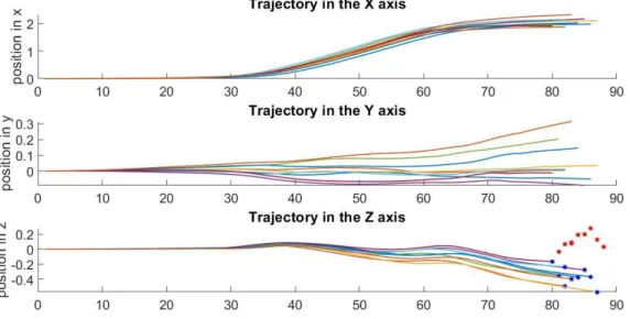
Since the subject moves in the direction of the X axis, with the Z axis being, ideally, the distance to the floor, the trajectory in the Z axis in the one that lets us visualize the position during the swing. This axis is also the one subjected to the biggest error, since once the integral previously discussed resets, all velocities are immediately set to zero, which forms a spike in the positions, as seen below.

(34)

22

Figure 2.6 Positions of the IMU, in meters, for each step, for the 3 axes. the blue points represent the end of the integral. the red represents the correction.

As we can see by the scale on the position axis, the trajectory in Y is much smaller, so, it can be ignored.

An adjustment to the program was made to remove the correction made to the velocity, and so, we obtain the following graphic:

Figure 2.7 Positions, in meters, in the 3 axes after removing the correction.

Finally, 2 other sets of scripts were created to evaluate the data: one to align all the steps of a single trial and average the position and angle of said trial, and another to calculate and evaluate the errors of the Z position. This last script also accumulated the error data of all the trials as they were being evaluated so a final graphic and comparison could be made in the end. All these can be seen the Chapter 4 of this document.

(35)

23

2.2.1. Data acquisition

Trials were made with 3 different subjects, 2 males and a female. Each trial consisted in several walks at 3 different speeds.

The device was placed in the right leg, and strapped with Velcro ties and tape, so it wouldn’t move or disconnect during trials, as shown in Figure 2.8. The IMU was positioned so that the direction of the walk would correspond to walking along the X axis, and that gravity would approximately be anti-parallel to the Z axis. The IMU was placed on top of the shoe, so the b frame would have the configuration showed. However, this method proved not entirely reliable, as the sensor may be disturbed by the movement of the toes inside the shoe, or get loose from its positioning. The

alternative method, used in latter trials, was to strap the IMU to a fix platform that would be fixated on the side of the shoe.

Figure 2.8 the device strapped to the leg (on the left) and the ideal positioning of the IMU axis (on the right)

The device was connected to the computer via USB cable, and the interface, seen below, read and wrote data in a .csv file, at a chosen frequency, that, for this project, was 80Hz.

Figure 2.9 Interface used for this project.

.

The results were stored at a designated folder. Each time the interface was opened, and new folder would be created, so, all trials for one person were stored into the same folder. The .csv files

(36)

24 were then uploaded to MATLAB, where the integrals within the main script would calculate all the necessary data for analysis, as well as creating all the graphs that will be shown in the next chapters.

(37)

25

3. Results

There are 3 types of data we can extract: the rotation matrix, the position, and the angle in relation to the floor. This information allows us to make a basic model of the gait. We’re going to start by analyzing the gait of a normal walk, and then proceed to the gait when walking up and down stairs.

3.1. Graphics

3.1.1. Raw data and integrals

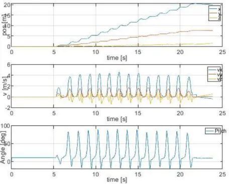
The following graphic (Figure 3.1 Figure 3.2) shows the data acquired by the device, linear acceleration and angular velocity, in the respective scaled units, m/s2 and rad/s. Analyzing the graphics, we can count the number of steps taken, but it’s very hard to take any conclusion of such data on its own. For that, it’s necessary to integrate the data, as has been discussed in previous chapters.

(38)

26

Figure 3.2 Raw data of the IMU, converted to standard units and divided per step

After the integrals were run, we have linear velocity and angle of the foot. Integrating the velocity once more, we get the relative position. To be noted that the initial position necessary to define any constants is the defined by the first few seconds, where the script calculates the gravity vector to form all frames. Whenever the foot hits the ground, a new frame is formed, as explained in previous chapters. For this experiment, it was only considered the rotations around the Y axis, since the angle values acquired from that correspond to the angle of the foot in relation to the axis (in this case, the 0 corresponded to the horizontal plane, and the rotation was clockwise, as shown below). The way the axis is positioned, a positive corresponds to the foot being rotated downwards (for example, when the foot leaves the ground), and a negative angle corresponds to the foot rotating upwards.

(39)

27

Figure 3.4 Integrated data, adapted to standard units

Finally, after dividing the data in steps, and aligning them, we can get a graphic of position and rotation, as well as being able to calculate their respective averages for each trial and subject.

3.1.2. Positions

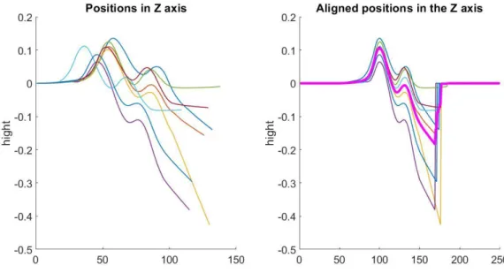
The graphic below shows an example of each step, in the z axis, the left image showing it as it’s calculated by the integral, and the right image, with each step being aligned by its first peak. The pink line shows the average z coordinate of all the steps. To be noted that, at the end of a step, the pink line is very irregular. That phenomenon is due to the fact that no step has the exact same length, so, when aligned, they end on different instants. Since the default of each aligned vector is 0, when averaging, those zeroes are counted into it, which results in that aspect, better visualized in Figure 3.6. The same phenomenon will happen when analyzing the foot angle.

(40)

28

Figure 3.5 Z axis positions for each step in one trial, and average of said steps

Figure 3.6 zoomed aligned z axis positions

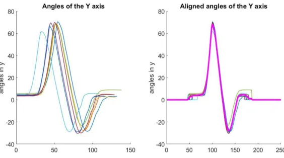
3.1.3. Foot angle in relation to the floor

The same can be done for the foot angle. Since the resting position is, ideally, relatively closer to zero than when calculating the Z axis positions, the error mentioned above isn’t as visible here.

(41)

29

Figure 3.7 ankle rotations in the Y axis for each step in one trial, and average of said steps

3.2. Analysis with different types of steps

3.2.1. Speed

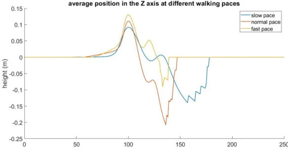
Each subject was asked to walk at 3 different paces: normal walk, slow pace, and fast march. Because the device has to be connected to the computer in real time, it was not safe or reliable to do run trials. These cannot be directly compared, i.e., within the code, because the steps have different velocities, as shown in Figure 3.8.

Figure 3.8 Average foot angle for different walking paces Foot angle at different walking speeds

(42)

30

Figure 3.9 average position in the Z axis for different walking paces

As it can be seen, each vector has substantially different lengths, as seen in how they peaks don’t align or in how the vectors end in very different instances. Because of that, when comparing the data at a same given instance, in practical terms, that instance is at a different stage of the gait, depending on the speed said gait was performed. Therefore, we can’t mathematically compare, or average steps taken at different walking speeds.

However, it is possible to average and compare different trials, as long as said trials are of the same walking speed, as will be showed in further chapters.

3.3. Limitations

3.3.1. Subjects and trials

The trials were taken with different subjects, walking the same corridor and same stairs. However, and despite a substantial effort to place the IMU on the same position, and have each subject walk at roughly the same velocity, there are clear differences between subjects, and even between trails taken on the same subject, but on different days. As such, the comparisons made between trials of different subjects can’t produce very accurate conclusions with the methods used.

3.3.2. Velocity correction and Z error

The 2nd degree integral, in order to have results, requires an initial velocity. Because the integral restarts each step, each new step requires a new initial condition. So, the scrip assumes the velocity on t = 0 in each step is 0. Since each step, by concept, starts with the foot on the ground, this assumption is not far off. However, the velocity is also never absolute 0, so, there’s always a small error to taken into account.

(43)

31 In the program, this error translates into a correction in the last state of each step, i.e., the last string of values. Those values are corrected so every step ends on |v| = 0, or the closest the algorithm can get it. When integrated into the position, this translates to sharp shifts in each step, particularly visible in the Z axis.

Another consequence of the 2nd degree integral is that there are 2 constants that are calculated, instead of 1. The first one is a normal constant that comes for integration. However, the constant becomes a first degree element, in mathematical terms, when it’s applied the 2nd_{integral. That}

translates to a steep slope (positive or negative) when plotting the Z axis position (it’s also visible in the other 2 axis, but the Z axis is both the most prominent and the most important for this project). That slope always forms in the last iteration of the position vector, so, in most calculations, it can be removed.

On the trials that were made in even terrain, it’s to be expected that the Z position in the beginning of a step would be the same as the end position, since the ground is at the same relative height. However, there’s a clear slope between those positions. The script attempts to correct this in the following step, when the integral resets.

3.3.3. Aligning steps

A script was made to align each step in one trial, excluding the first and last. The first and last step as excluded because it’s when the subject start and stops the gait, respectively, so, these steps have added forces that compromise the data.

The script consists in detecting the peaks of each step, and dislocate the location of the first one (along with all the vector) to a specific location (the 100th position was chosen for convenience), for both the Z axis position and the ankle angle, so that all peaks are located in the 100th position, meaning they’re aligned in relation to one another. This allows to calculate the average step for a subject.

Because each step isn’t exactly the same length or take the same time, each z vector ends at a slightly different instant. As such, the error in the average towards the end is very visible (as shown on the example in figure 9 below). Because of how the script was written, the vector of the aligned steps goes back to zero when the step ends (resulting in those sharp lines), which makes the average not entirely accurate. The same can be done for the ankle angle. Because the resting position is a lot closer to zero, in relative dimensions, than when calculating the Z axis positions, the error mentioned above isn’t as visible.

(44)

(45)

33

4. Discussion

4.1. FSR detection

A new script was written to detect the FSR signal within the data. The main script was built so there would be a vector (step_up) that would be made of zeros. This new FSR script would turn certain zeros into ones, according to the detection in the data. The main script would then use this set of ones to differentiate one step from another.

At first, the script was written so any instance where a certain FSR was pressed, it would turn a zero in that instance into a one, as shown in Figure 4.1. However, that approach was less than ideal, since there were several instances where the foot was on the ground (so the FSR was active) where the foot was still moving, particularly during the initial contact and take off, because, for practical effects, the integral does not count those iterations in when calculating position and angle, so, that data is lost. Ideally, in order to minimize data loss, the step_up vector would have no iterations, so that all data was counted, but that is not practical, because the program needs to know when a new step starts so it can form a new frame.

The next best option is one iteration, so, in practical terms, only 1/80 of a second (the time one iteration has, considering the data was taken at 80Hz) is lost.

This means it’s necessary a code that identifies only one point of the FSR peaks during a trial, and marks that point as a one.

For convenience, the point chosen was the maximum value of each peak, as shown Figure 4.2.

(46)

34

Figure 4.2 FSR detection using the final method

4.2. Subjects

4.2.1. Position in the Z axis

Subject 1

Figure 4.3 Ideal Z axis position during the gait. Adapted from [33].

The figure above represents what the ideal results should be, according to the literature, for the chosen defined gait of it being between heel-strikes. As such, we’ll be comparing all the results below to this one.

(47)

35

Figure 4.4 Position, in the Z axis, of subject 1's foot, while walking at a slow pace

(48)

36

Figure 4.6 Position, in the Z axis, of subject 1's foot, while walking at a fast pace

It can be observed that, as the subject’s pace increases, so does the average slope between the beginning and end of a step.

Despite that, the shape of the curve is what is to be expected in all speeds.

Subject 2

(49)

37

Figure 4.8 Position, in the Z axis, of subject 2's foot, while walking at a normal pace

For the second subject, there’s no clear difference (other than the length of the vectors) between the different gait speeds.

However, close examination can tell us that, while the rough shape of the curve is similar, the curve at the fastest speed loses the ideal shape, giving into the slope of the error.

(50)

38 Subject 3

Figure 4.10 Position, in the Z axis, of subject 3's foot, while walking at a slow pace

(51)

39

With the third subject, contrary to subject 1, as the gait speed increases, the slope between the beginning and end of a step becomes less noticeable. It can also be seen that it’s the normal pace curve the one whose less shaped like the ideal result.

As it can be observed, there’s no clear pattern regarding the accuracy of the gait in relation to the speed of the walk. The vectors of the trials with higher gait speed are shorter, as it’s expected, but the average displacement (for reference, both the beginning and end of a step should be 0, on average) doesn’t follow any fort of pattern.

However, the general shape of the curve matches what’s to be expected from the literature, as seen in Figure 4.3 Ideal Z axis position during the gait. Adapted from [33].Figure 4.3, despite an overall clear difference in height between the first and second peaks, that shouldn’t, ideally, exist.

(52)

40

4.2.2. Foot angle in relation to the floor

As for the foot angle, the image below, depicting the ideal foot angle during a gait, is what it will be used for the comparison to the literature.

Figure 4.13 Expected shape of the curve of the foot angle in relation to the floor. Adapted from [34].

To be noted that, for the case described in literature, the angle was measured under an inverted axis when compared to the data acquired in this project, so, all results below should, ideally, be a negative of the image seen above.

To also be noted that the resting angle varies from subject to subject, due to the positioning of the IMU sensor o top of the shoe. As we depict each subject, the resting angle for that subject will be disclosed.

Subject 1

Figure 4.14 Foot angle of subject 1's foot, while walking at a slow pace Average foot angle at a slow pace

(53)

41

Figure 4.15 Foot angle of subject 1's foot, while walking at a normal pace

Figure 4.16 Foot angle of subject 1's foot, while walking at a fast pace

As it can be seen in all graphs, the foot angle when the foot is at rest, on the ground, is 20.3604º. Overall, there isn’t much difference between all the different speeds. They all closely resemble both the ideal results and each other. The only real difference is the length of the vectors.

Average foot angle at a normal pace

(54)

42 Subject 2

Figure 4.17 Foot angle of subject 2's foot, while walking at a slow pace

Figure 4.18 Foot angle of subject 2's foot, while walking at a normal pace Average foot angle at a slow pace

(55)

43

Regarding this subject, the resting foot angle is 9.4593º.

Like the last subject, this too doesn’t show itself different from the model of reference. the shape of the curve is exactly what was to be expected.

One detail to notice is that, comparing to subject one, subject 2’s results regarding the foot angle are slightly more consistent overall (i.e., while in subject 1, the lines that made up each trial average were visible, meaning they were further from the average, in subject 2, they’re hardly noticeable, meaning they’re overlapping each other much more).

Subject 3

Figure 4.20 Foot angle of subject 3's foot, while walking at a slow pace Average foot angle at a fast pace

(56)

44

Figure 4.21 Foot angle of subject 3's foot, while walking at a normal pace

Subject 3’s resting foot angle is 4.5220º.

Like the other subjects, the results match the ideal model used very closely. All the curves showed are to be expected, and there’s no clear outlier in any of the graphs.

Overall, the measurements of the angle were much more consistent and accurate than the ones made form the position, and the results are as expected. There doesn’t to be any major difference (apart from the starting angle) between subject, or when comparing the different speeds. This

difference in the starting angle are due to the positioning of the IMU. Because it was placed on top of the subject’s shoe, the angle will vary depending on the type of footwear the subject was using during the trials.

That being said, the results are within what was to be expected, according to the literature, as seen in Figure 4.13.

Average foot angle at a normal pace

(57)

45 It’s also important to note that all the trials of the same subject were made on the same day, with the IMU in the same position, so that the data could be compared mathematically.

4.3. Inter subject analysis

Although we can’t accurately compare the position and angle, we can compare the error that results from it.

4.3.1. Error within the same step

Between the beginning and the end of a step, of flat ground, the Z position value should theoretically be the same (again, not counting the mathematical error that comes from the velocity adjustment), so, the difference between the value measured in the first instance and the last, on the same step, should be 0.

From that, this error was calculated to measure how different that is from the ideal value.

Figure 4.23 Error within a step for subject 1. Slow pace; Average error: -0.0911. standard deviation: 0.1083. Normal pace; Average error: -0.1972. standard deviation: 0.1228.

(58)

46

Fast pace; Average error: -0.2275. standard deviation: 0.0821.

The 3 subject present wildly different results regarding this type of error. The average error doesn’t seem to have a pattern, getting closer and further from 0, regardless of velocity. To be noted that, in all 3 subjects, the average farthest away from 0 is always the walk at normal speed (in red).

However, regarding standard deviation, for subjects 1 and 2, increases with the increase of speed. This can be due to the fact that the position vectors for the fast pace walks are smaller, because it takes less time to complete a step, so, the discrete nature of the data leaves larger gaps that can

(59)

47 translate to error. But said conclusions can’t be confirmed without more subjects, sense the results of subject 3 don’t follow the same pattern.

4.3.2. Error between steps

This error is defined as the difference on position (on the Z axis) between the last instance of the previous step (not counting the correction error from the velocity adjustment) and the first instance of the next. Theoretically, when the data was taken on a flat surface, this difference should be 0. It should also be 0 for the trails walking upstairs, because the foot lands and leaves the same step, which is a flat surface as well.

Figure 4.26 Error between steps, for subject 1. Slow pace; Average error: -0.0729. Standard deviation: 0.1127. Normal pace; Average error: -0.1695. Standard deviation: 0.1532.

(60)

48

Figure 4.27 Error between steps for subject 2. Slow pace; Average error: -0.2215. standard deviation: 0.0685. Normal pace; Average error: -0.2338. standard deviation: 0.0755.

Figure 4.28 Error between steps for subject 3.

Slow pace; Average error: -0.1107. Standard deviation: 0.0831. Normal pace; Average error: -0.1187. Standard deviation: 0.1854. Fast pace; Average error: -0.0107. Standard deviation: 0.1185.

Once again, a pattern can’t be observed regarding the average error. As it was in the previous case, for subjects 1 and 2, the standard deviation increases as the gait velocity increases. However, that doesn’t translate to subject 3.