Deep learning for multi-class skin lesion diagnosis

Universidade de Aveiro Departamento de Eletrónica,Telecomunicações e Informática 2020

Fábio

Santos

Aprendizagem profunda para o diagnóstico de

múltiplas classes de lesões de pele

Deep learning for multi-class skin lesion diagnosis

“Our intelligence is what makes us human, and AI is an extension of that quality”

— Yann LeCun Universidade de Aveiro Departamento de Eletrónica,Telecomunicações e Informática

2020

Fábio

Santos

Aprendizagem profunda para o diagnóstico de

múltiplas classes de lesões de pele

Deep learning for multi-class skin lesion diagnosis

Universidade de Aveiro Departamento de Eletrónica,Telecomunicações e Informática 2020

Fábio

Santos

Aprendizagem profunda para o diagnóstico de

múltiplas classes de lesões de pele

Deep learning for multi-class skin lesion diagnosis

Dissertação apresentada à Universidade de Aveiro para cumprimento dos requisitos necessários à obtenção do grau de Mestre em Engenharia Informática, realizada sob a orientação científica do Doutor Filipe Miguel Teixeira Pereira da Silva, Pro-fessor auxiliar do Departamento de Eletrónica, Telecomunicações e Informática da Universidade de Aveiro, e da Doutora Pétia Georgieva, Professora auxiliar do Departamento de Eletrónica, Telecomunicações e Informática da Universidade de Aveiro.

o júri / the jury

presidente / president Prof. Doutor Luís Filipe de Seabra Lopes

Professor Associado do Departamento de Eletrónica, Telecomunicações e Informática da Univer-sidade de Aveiro

vogais / examiners committee Prof. Doutor João Paulo Morais Ferreira

Professor Adjunto do Instituto Superior de Engenharia de Coimbra

Prof. Doutor Filipe Miguel Teixeira Pereira da Silva

Professor Auxiliar do Departamento de Eletrónica, Telecomunicações e Informática da Universi-dade de Aveiro

agradecimentos /

acknowledgements Quero deixar um grande agradecimento ao orientador Filipe Silva e à co-orientadoraPétia Georgieva por toda a dedicação e apoio prestado no desenvolvimento desta dissertação. Quero também agradecer ao Professor Vitor Santos (DEM) e à equipa do LAR do departamento de Engenharia Mecânica, pela disponibilidade dos recur-sos computacionais necessários para a conclusão desta dissertação. Por fim, quero deixar um especial agradecimento aos meus amigos e família que desde cedo me deram o suporte necessário para que seja bem sucedido nos trabalhos que realizo.

Palavras Chave classificação de lesões de pele, classificação de múltiplas classes, aprendizagem pro-funda, rede neuronal convolucional, aprendizagem por transferência, desempenho de generalização.

Resumo Aprendizagem profunda é um ramo de aprendizagem automática que tem crescido rapidamente e que tem sido usada em problemas relacionados com imagem médica, tais como a deteção de cancro da pele. Durante muito tempo, o diagnóstico de lesões de pele através de imagens clínicas usando aprendizagem profunda era algo considerado inalcançável. No entanto, avanços recentes em redes neuronais pro-fundas permitiram obter resultados de referência em tarefas de classificação. Além disto, existe uma necessidade crescente de sistemas capazes de automatizar este tipo de diagnósticos para reduzir a taxa de mortalidade causada por cancro da pele. Isto proporcionará suporte a dermatologistas no processo de decisão e a pacientes que não tenham fácil acesso a médicos especialistas. Esta dissertação apresenta uma abordagem sistemática tendo em vista o desenvolvimento de um classificador multiclasse (8 classes) para o diagnóstico automático de lesões de pele. O estudo visa analisar um conjunto de metodologias de aprendizagem profunda que permi-tam responder a questões relacionadas com a sua eficácia. Os resultados indicam que os modelos pre-treinados, baseados em arquiteturas convolucionais, têm um impacto significativo no desempenho desde que sejam devidamente reaproveitados usando aprendizagem por transferência. Este trabalho proporciona uma visão mais clara sobre a influência de diferentes métodos na capacidade de generalização des-tes modelos. Neste contexto, o impacto de diferendes-tes métodos de processamento de imagem para o aumento de dados é revelado. Por um lado, o balanceamento de classes através do aumento de dados offline permite melhorar significativamente o desempenho de classes sub-representadas. Por outro lado, o aumento de dados on-line traz melhorias consideráveis na redução do sobreajuste (overfitting). Adici-onalmente, é fornecida uma análise prática de métodos de ensemble no contexto do diagnóstico de lesões de pele. Os resultados obtidos com um modelo pre-treinado e com o ensemble superam o atual estado da arte da competição ISIC 2019, com uma acurácia balanceada (balanced accuracy) de 0,815 e 0,846, respetivamente. Finalmente, foram feitas experiências com diferentes algoritmos para detetar dados que não pertencem à distribuição que resulta das 8 classes originais. Os resultados obtidos contribuem para a compreensão da eficácia destes métodos no contexto de classificadores de lesões de pele.

Keywords skin lesion diagnosis, multi-class classification, deep learning, convolutional neural network, transfer learning, generalization performance.

Abstract Machine learning, more specifically, deep learning is a fast-growing field that is be-ing used for multiple medical imagbe-ing related problems, such as the early detection of skin cancer. For a long time, automated diagnosis of skin lesions from clinical images through deep learning was considered to be out of reach. However, recent advancements in deep neural networks allowed it to achieve state-of-the-art results on classification challenges and they have the potential to change the landscape of dermatology care. Moreover, there is a growing need for classification systems to reduce fatality rates of skin cancer by providing support for both dermatologists in the decision-making process and for patients that do not have access to expert physicians. This dissertation presents a systematic approach towards an multi-class (8 classes) deep learning classifier of skin lesions for the ISIC 2019 benchmark chal-lenge. It attempts to study major open research points related to the effectiveness of state-of-the-art deep learning methods. The results indicate that recent CNN architectures can have a significant impact on the overall performance of deep learning based classifiers. However, these pre-trained models should be carefully re-purposed towards skin lesion classification through transfer learning methods. This work provides insight into major ways of improving the generalization per-formance of deep learning models towards skin lesion diagnosis. In this context, the impact of different image processing augmentation methods for offline and online data augmentation is studied. On the one hand, class balancing through offline data augmentation can significantly improve the generalization performance of underrepresented classes. On the other hand, online data augmentation brings considerable improvements towards overfitting reduction. Furthermore, this work provides a practical analysis of ensembles in the context of skin lesion diagnosis. Both the single model and the ensemble-model approach outperform the current state-of-the-art for the ISIC 2019 challenge, with a balanced multi-class accuracy of 0.815 and 0.846, respectively. Finally, experiments were made with different ways to detect out of training distribution data. The results contribute towards the understanding of the effectiveness of out-of-distribution detection methods in the context of deep learning based skin lesion classifiers.

Contents

Contents i List of Figures v List of Tables ix Acronyms xi 1 Introduction 1 1.1 Background . . . 1 1.2 Motivation . . . 2 1.3 Objectives . . . 4 1.4 Outline . . . 4

2 Methods and Materials 5 2.1 Artificial Neural Networks . . . 5

2.1.1 Activation Functions . . . 6

2.1.2 Optimization Algorithms . . . 7

2.1.3 Initialization Strategies . . . 9

2.2 Convolutional Neural Networks . . . 10

2.2.1 CNN Fundamentals . . . 10

2.2.2 State-of-the-art CNN Architectures . . . 11

2.3 Transfer Learning . . . 19

2.4 The Bias and Variance Tradeoff . . . 21

2.4.1 Underfitting Solutions . . . 21

2.4.2 Overfitting Solutions . . . 22

2.5 Ensemble Learning . . . 23

2.5.1 Combine Models Trained on Different Data . . . 23

2.5.2 Combine Models Trained on Different Conditions . . . 24

2.6 Performance Metrics . . . 24

2.7 Out of Training Distribution Detection . . . 27

3 Skin Lesion Diagnosis 29 3.1 eHealth and mHealth Applications . . . 29

3.2 Hand-crafted Image Processing Methods . . . 31

3.2.1 Lesion Segmentation . . . 31

3.2.2 Feature Extraction . . . 31

3.2.3 Disease Classification . . . 32

3.3 Deep Learning for End-to-end Classification of Skin Lesions . . . 33

3.3.1 Transfer Learning Approaches . . . 33

3.3.2 Learning from Scratch Approaches . . . 39

3.4 Challenges and Opportunities of Deep Learning Methods . . . 40

3.4.1 Interpretability . . . 40

3.4.2 Data Limitations . . . 41

3.4.3 Out of Training Distribution Test Data . . . 42

3.4.4 Hardware Limitations . . . 42 3.4.5 Workflow Integration . . . 43 4 Experimental setup 45 4.1 Experimental Scope . . . 45 4.2 Data Representation . . . 47 4.2.1 Description . . . 47 4.2.2 Class Imbalance . . . 51 4.2.3 Unknown Class . . . 52 4.3 Data Preprocessing . . . 53 4.4 Data Augmentation . . . 55 4.5 Data Split . . . 59 4.6 Hardware . . . 60 4.7 Software . . . 61

5 Pre-trained Model Choice and Parameter Optimization 63 5.1 Pre-trained Model Choice . . . 63

5.1.1 Freeze the Convolutional Layers . . . 65

5.1.2 Extraction and Fine-tuning of Convolutional Layers . . . 66

5.2 Hyperparameter Optimization . . . 69

5.2.1 Varying the Batch Size . . . 70

5.2.2 Varying the Number of Epochs Before Fine-Tuning . . . 71

5.2.4 Varying the Learning Rate Scheduler’s Patience . . . 75

5.2.5 Applying Regularization Techniques . . . 77

5.3 Results Discussion . . . 78

6 Improving Model Generalization Performance 81 6.1 Data Study . . . 81

6.1.1 Impact of Dataset Size . . . 82

6.1.2 Impact of Augmentation Techniques . . . 86

6.1.3 Impact of Class Balancing through Data Augmentation . . . 90

6.2 Model Ensemble . . . 94

6.3 Out of Training Distribution Detection . . . 97

6.3.1 Softmax Threshold . . . 98

6.3.2 Out-of-DIstribution detector for Neural networks (ODIN) . . . 100

6.3.3 Outlier Class . . . 101

6.3.4 Approach Comparison . . . 102

6.4 Results Discussion . . . 103

7 Conclusion 105 7.1 Discussion . . . 105

7.2 Limitations and Future Work . . . 106

7.3 Contributions . . . 108

List of Figures

2.1 Example of a feedforward fully-connected artificial neural network taken from Michael Nielsen [28]. . . 6 2.2 Example of max pooling operation with a 2×2 filter and a stride of 2 [38]. . . 11 2.3 Custom Convolutional Neural Network (CNN) architecture used to classify digits from the

Modified National Institute of Standards and Technology (MNIST) dataset taken from Michael Nielsen [28]. . . 11 2.4 Architecture of the VGG16 CNN [42]. . . 12 2.5 Skip connection, the building block of residual neural networks. Taken from He et al. [39]. 13 2.6 A block from DenseNet with five layers each with an expansion of 4 . . . 14 2.7 Model scaling methods as presented by Tan et al. [44]. . . . 15 2.8 Inception module from the InceptionV1 architecture [45]. . . 16 2.9 Inception module A (left), B (middle) and C (right) of the InceptionV2 architecture [46]. 17 2.10 Inception module A (left), B (middle) and C (right) of the InceptionResNet (V1 and V2)

architecture [48]. . . 17 2.11 Transfer learning strategies . . . 20 2.12 Influence of model complexity on the bias and variance. . . 21 2.13 ROC (Receiver Operating Characteristic) curve for a multi-class classification problem

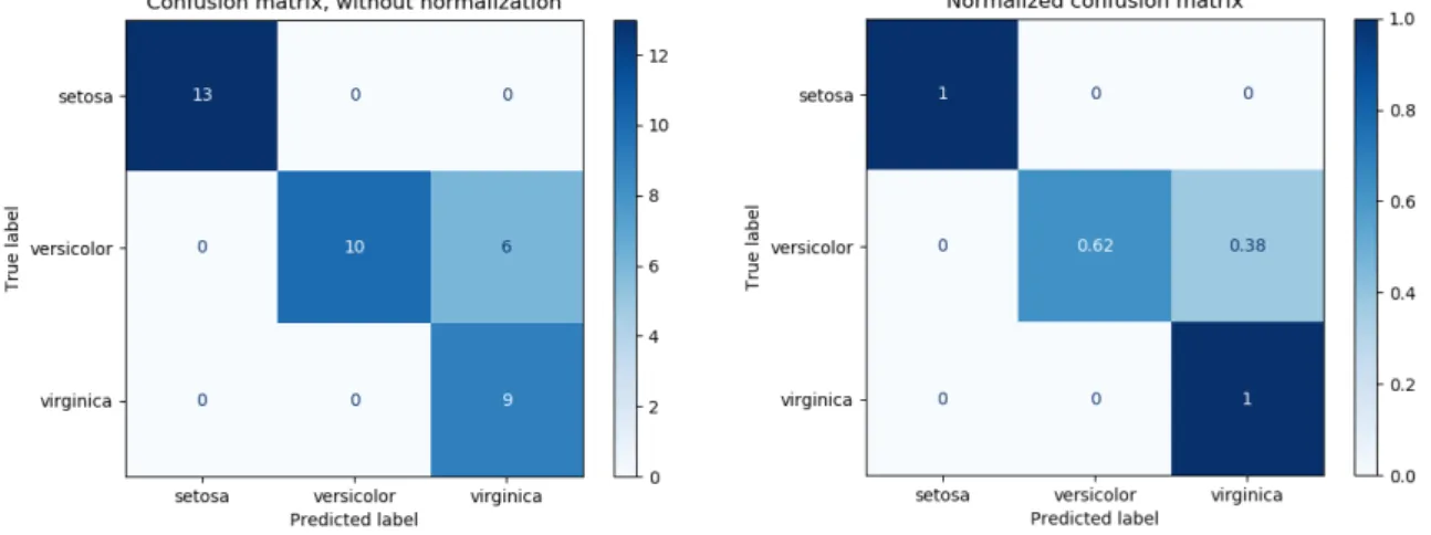
with micro and macro averages to summarize all classes. Taken from scikit-learn. . . 26 2.14 Non-normalized vs. normalized confusion matrix for a 3 class classification problem. Taken

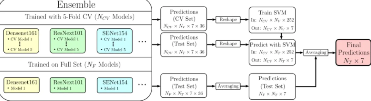
from scikit-learn. . . 26 3.1 Contribution of each classification method to the total number of dermoscopic studies

according to the review paper of Prabhu et al. [9]. . . . 33 3.2 The evaluation strategy for the generation of final predictions of Gessert et al. [20]. . . . 36 4.1 Hierarchical organization of skin lesions. . . 48 4.2 HAM10000 sample filtering process. . . 49 4.3 Samples from ISIC 2019 training data for the 8 known categories. . . 50

4.4 Class distribution of International Skin Imaging Collaboration (ISIC) 2019 challenge training dataset. . . 51 4.5 Weights for each class of the weighted cross-entropy loss function in the ISIC 2019 training

dataset. . . 52 4.6 Randomly chosen samples from the dataset created for the "unknown" class. . . 53 4.7 Examples of shear augmentations. . . 56 4.8 Examples of tilt augmentations from forward the x-axis (middle) and y-axis (right). . . . 56 4.9 Examples of skew augmentations towards different corners of the image either on the x- or

y-axis. . . 57 4.10 Example of an distortion applied as an augmentation method. . . 57 4.11 Examples of image processing augmentation techniques used in Chapter 6. . . 58 4.12 Sample distribution used for the train, validation and test sets across 9 different classes. . 60 4.13 Deeplar, the computer used for the experiments of the presented research work. . . 61 5.1 Three samples of the test set along with their respective softmax probabilities. . . 65 5.2 Comparison of pre-trained models with frozen convolutional base . . . 66 5.3 Comparison of pre-trained models with fine-tuned convolutional base . . . 67 5.4 Ground truth samples, prediction samples, and correct prediction samples across different

classes in the test-set using the fine-tuned DenseNet201 model. . . 69 5.5 Batch size vs train and validation Balanced Multi-class Accuracy (BMA) over epochs for

the fine-tuned DenseNet201 trained with 5000 samples. . . 71 5.6 Number of epochs before the fine-tuning process vs train and validation BMA over epochs

for the fine-tuned DenseNet201 trained with 5000 samples. . . 72 5.7 Learning rate used to train the classifier before the fine-tuning process vs BMA for the

fine-tuned DenseNet201 trained with 5000 samples. . . 73 5.8 Fine-tuning learning rate vs train and validation BMA for the fine-tuned DenseNet201

trained with 5000 samples. . . 73 5.9 Influence of the fine-tuning learning rate on train and validation BMA over epochs for the

DenseNet201 trained with 5000 samples. . . 74 5.10 Initial fine-tuning learning rate vs the learning rate over epochs for the DenseNet201 trained

with 5000 samples. . . 75 5.11 Initial fine-tuning learning rate vs validation loss over epochs for the DenseNet201 trained

with 5000 samples. . . 75 5.12 Influence of the learning rate scheduler’s patience on train and validation BMA over epochs

for the DenseNet201 trained with 5000 samples. . . 76 5.13 Influence of the learning rate scheduler’s patience on the learning rate over epochs for the

5.14 L2 regularization parameter vs train and validation BMA for the fine-tuned DenseNet201 trained with 5000 samples. . . 78 5.15 Dropout rate vs train and validation BMA for the fine-tuned DenseNet201 trained with

5000 samples. . . 78 5.16 Confusion matrix of the fine-tuned DenseNet201 pre-trained model, trained on 5000 ISIC

2019 samples. . . 79 5.17 Confusion matrix of the hyperparameter optimized and fine-tuned DenseNet201 pre-trained

model, trained on 5000 ISIC 2019 samples. . . 80 6.1 Different hyperparameter tuned DenseNet pre-trained models trained with 5000 samples

vs BMA on train, validation and test sets. . . 83 6.2 Number of training samples vs train and validation BMA for the DenseNet201 pre-trained

model. . . 83 6.3 Number of training samples vs train and validation BMA over epochs for the DenseNet201

model. . . 84 6.4 Influence of the number of samples on the learning rate over epochs for the DenseNet201

model. . . 84 6.5 Different hyperparameter tuned DenseNet pre-trained models trained with 20518 samples

vs BMA on train, validation and test sets . . . 85 6.6 Confusion matrix of the hyperparameter optimized and fine-tuned DenseNet121 pre-trained

model trained with the full unbalanced training dataset. . . 86 6.7 BMA of train, validation and test sets of different offline data augmentation groups with

the DenseNet121 trained on 20518 balanced samples. . . 88 6.8 BMA of the train, validation and test sets of different combinations of offline and online

data augmentation modes with a hyperparameter tuned DenseNet121 trained on 20518 balanced samples. . . 89 6.9 BMA of train, validation and test sets of different online data augmentation groups with

the DenseNet121 trained on 20518 unbalanced samples (no offline data augmentation). . 90 6.10 Comparison of the BMA of balanced and unbalanced datasets with 20518 samples for

the train, validation and test sets using the hyperparameter optimized and fine-tuned DenseNet121 pre-trained model. . . 91 6.11 Comparison of the accuracy of balanced and unbalanced datasets with 20518 samples for

the train, validation and test sets using the hyperparameter optimized and fine-tuned DenseNet121 pre-trained model. . . 92 6.12 Comparison of train, validation and test BMA and accuracy scores for different balanced

6.13 Confusion matrix of the hyperparameter optimized and fine-tuned DenseNet121 pre-trained model, trained with the balanced and oversampled ISIC 2019 dataset with 83432 samples. Online data augmentation was turned on during training with augmentation group 1. . . 94 6.14 Confusion matrix of the ensemble composed with the best 3 pre-trained models. . . 97 6.15 Comparison of different top-1 softmax threshold values for the detection of out of training

distribution samples from the test set. . . 99 6.16 Confusion matrix of the test set predictions on the hyperparameter tuned DenseNet121

trained with 8 classes where out of distribution samples are identified using a top-1 softmax threshold of 0.7. . . 100 6.17 Confusion matrix of the test set predictions on the hyperparameter tuned DenseNet121

trained with 8 classes where out of distribution samples are identified using the ODIN detector. . . 101 6.18 Confusion matrix of the test set predictions on the hyperparameter tuned DenseNet121

List of Tables

2.1 Models comparison on the ImageNet dataset. . . 18 4.1 Samples per category of skin lesion, for the "unknown" class. . . 53 6.1 BMA and Accuracy of different models and ensembles for 8-class classification of skin lesions. 96 6.2 Comparison of BMA and accuracy scores on the test set for the different methodologies to

detect out of training distribution samples. . . 102 6.3 BMA and accuracy on the test set for the different models created throughout this work. 103 6.4 Approach comparison with state-of-the-art approaches on 8- and 9-class classification for

Acronyms

ANN Artificial Neural Network

CNN Convolutional Neural Network

GAN Generative Adversarial Networks

SVM Support Vector Machine

CPU Central Processing Unit

GPU Graphics Processing Unit

TPU Tensor Processing Unit

RAM Random Access Memory

FLOPS FLoating point Operations Per Second

TP True Positive

TN True Negative

FP False Positive

FN False Negative

TPR True Positive Rate

TNR True Negative Rate

FPR False Positive Rate

PPV Positive Predictive Value

NPV Negative Predictive Value

AUC Area Under Curve

ROC Receiver Operating Characteristic

BMA Balanced Multi-class Accuracy

LAR Laboratory for Automation and

Robotics

ISIC International Skin Imaging

Collaboration

ILSVRC ImageNet Large Scale Visual Recognition Competition

MNIST Modified National Institute of Standards and Technology

HAM10000 Human Against Machine with 10000

images

ODIN Out-of-DIstribution detector for Neural

networks

TDS Total Dermoscopic Score

SCC Squamous Cell Carcinoma

CHAPTER

1

Introduction

In this chapter some background will be given for the problem statement, as well as the motivation and objectives behind this work.

1.1 Background

Skin cancer is the out-of-control growth of abnormal cells in the outermost skin layer, caused by mutations triggered within the genetic code [1]. These mutations lead the skin cells to multiply rapidly and form malignant tumors. It is currently the most common type of cancer [2] with melanoma being the most deadly form that accounts for about 75% of skin cancer deaths, even though it only represents 5% of all skin cancer cases [3]. Other forms of skin cancer such as the Basal Cell Carcinoma (BCC) or the Squamous Cell Carcinoma (SCC) are not as deadly but are much more common. BCCs are the most common type of skin cancer and have the potential to disfigure the skin and become dangerous [2]. Similarly, SCCs are the second most common form of this decease and, if left untreated, can destroy nearby healthy tissue, spread to other parts of the body, and eventually lead to death [1].

A recent study observed that in the United States of America alone, there are 5.4 Million new cases of skin cancer every year [2]. However, a bigger problem is that the incidence rates of skin cancer keep rising with currently 1 in 5 persons developing skin cancer until the age of 70 [1]. In Europe, melanoma incidence rates also manifest heavily, as each year 100000 people are diagnosed with melanoma, and approximately 22000 people die annually from this form of skin cancer [4].

Even though skin cancer can be deadly in late stages, if detected early there is a high chance of survival. For example, there is a 23% chance of surviving a melanoma case if detected in the late stages, but if detected early, the five-year survival rate (i.e., percentage of people alive after five years) is approximately 98% [1]. Therefore, the early detection of skin cancer is a top priority in order to increase the overall survival rate of the population.

Skin cancer can be detected by dermatology professionals by performing a visual exam-ination of skin lesions. However, some authors believe that the dermatologist’s experience

directly impacts his diagnostic accuracy [5], which implies that different physicians might make a different diagnosis for the same lesion. Some works have corroborated this in practice. For example, Argenziano et al. in their study noted that dermatologists have a 65% to 80% interval of accuracy in melanoma diagnosis [6]. However, this rate can be overall increased with the supplement of dermatoscopic images [7]. These type of images are taken with a special high-resolution and magnifying camera in a controlled light environment, where reflections on the skin are minimized which causes deeper skin layers to be visible.

Automated diagnosis of skin lesions through the dermatoscopic and non-dermatoscopic images has been achieving significant progress over the years, as demonstrated by some state-of-the-art surveys [8][9][10]. Typically, computer vision algorithms are used to analyze images and extract structural information [11], such as the ABCDE (Asymmetry, Border, Color, Dermoscopic structure, and Evolving) rule [12] or the CASH (color architecture, symmetry, and homogeneity) algorithm. These algorithms are then integrated within systems to provide quantification of features for physician assessment and for provisional diagnosis.

However, recent studies show that more complex structures called Convolutional Neural Networks (CNNs) are being applied to classify skin lesions with remarkable performance in comparison to human experts [3][5][13]. Moreover, the interest on this topic is well demonstrated by the large number of papers related to deep learning published in the context of the ISIC challenges [14]. This paradigm shift became apparent in 2016, for the International Symposium on Biomedical Imaging (ISBI) benchmark challenge towards melanoma detection. From 25 teams, all of them employed CNNs, instead of hand-crafted computer vision algorithms or other machine learning methods [15].

CNNs are a type of deep learning architecture. In turn, deep learning refers to computa-tional models composed of multiple processing layers capable of learning representations of data with multiple levels of abstraction [16]. Deep learning topologies have a considerable advantage over traditional Artificial Neural Networks (ANNs), namely, they do not require the selection of an appropriate set of features from which the algorithm learns. This task involves extracting knowledge or information which is implicit in the raw data, requiring careful engineering and knowledge of the problem domain. Some developments allowed CNNs to emerge as an feasible approach to computer vision classification problems, such as the use of the Graphics Processing Unit (GPU) to speedup computations and the development of high-level software modules to train deep neural networks.

1.2 Motivation

Current implementations of deep learning models for skin lesion diagnosis still present major challenges to overcome. The biggest one is the requirement for large amounts of training data in order to achieve superior performance to other methods. However, publicly available datasets for medical imaging related problems are typically small compared to the needs of training a deep CNN from scratch [17]. Even though training a model from scratch is a feasible approach for big datasets (e.g., ImageNet [18]), alternative approaches like transfer learning present an workaround for small datasets. Transfer learning is a technique in which

one can leverage the knowledge obtained from a deep model previously trained on a large labelled dataset towards a new classification task [19]. Furthermore, transfer learning does not require as much machine learning expertise as designing a model from scratch, tuning its hyperparameters, and making thorough discussions about the results. For this reason, in recent years, transfer learning based approaches have become prevalent for automated skin lesion diagnosis [3][5][20][21].

However, some questions remain open in the context of transfer learning based models for skin lesion classification, namely: "Which strategy should one chose to train these transfer

learning based models?", "What pre-trained models and architectures bring benefits to the classification of skin lesions?", "How does model depth affects the performance of transfer learning based deep learning models?", and "How can hyperparameter optimization help transfer learning based approaches achieve higher generalization performance?".

In addition to transfer learning, a commonly used method to ease the requirement for large amounts of data is data augmentation [22]. This term involves a large range of methodologies which aim to create synthetic samples that allows a model to attain better generalization performance. Furthermore, skin lesion datasets are often highly unbalanced which can cause the model to optimize its results for overrepresented classes. Several approaches attempt to solve this issue by class balancing samples through data augmentation [23]. However, some questions remain open about its usage, namely: "Can class balancing through data

augmentation help increase generalization performance of underrepresented classes?", "What is the influence of dataset size on generalization performance?", "What is the influence of data augmentation in deep learning for small datasets?", "Which data augmentation image processing algorithms should one apply for the problem of skin lesion classification?".

Moreover, the top approaches towards skin lesion classification systems of benchmark challenges such as the ISIC 2019 [24], usually employ model ensembling methods in order to attain better generalization performance [21] [25] [26]. However, one could ask the following open questions: "How can one employ these type of techniques to get meaningful improvements

on the generalization performance?", "Do the obtained improvements justify the disadvantages of using these types of methods?", and "Are these approaches practical to be deployed into the clinical workflow?". Ultimately, the goal of all of these questions is to further improve

generalization performance of deep learning models.

However, in a production environment, samples of skin lesions may be taken under far different conditions from their training dataset (e.g., lighting conditions) or might not be part of the original training categories. Work in this field reports that deep learning models are highly sensitive to a different sample distribution from their original training distribution [14][27]. This is a known problem of deep learning models, which out-of-distribution detection methods attempt to solve. Ideally, these types of methods could flag out-of-distribution samples for further inspection of a dermatologist, which would ultimately augment his capabilities, rather than replace them. However, some questions remain open towards this methods in the context of skin lesion classification: "What methods can one use to detect out of training distribution

1.3 Objectives

A strong assumption can be made that the recent advancements of deep learning based methods have the potential to change the landscape of skin lesion diagnosis because it would minimize the time it takes to detect skin cancer cases. However, one must first closely study the impact of the presented problems and the different strategies to deal with them, as it will likely lead to useful insights and contributions to the current state-of-the-art methods. Therefore, the following key objectives are highlighted for this work:

• Study the impact of transfer learning methodologies, pre-trained model architectures and parameters in the context of skin lesion classification;

• Study the impact of data augmentation, class balancing, and ensembling techniques as methods to improve performance for skin lesion classification;

• Experiment with different strategies to identify out of training distribution samples from the test set;

• Create a comprehensive approach for the ISIC 2019 benchmark challenge that provides some insight into ways of optimizing generalization performance.

1.4 Outline

Considering the presented objectives, the remainder of this dissertation is organized as follows: • Chapter 2 introduces the reader to deep learning concepts and techniques relevant to the current state-of-the-art methods which automate skin lesion diagnosis using deep learning;

• Chapter 3 provides an overview of recent progress in the automated diagnosis of skin lesions;

• Chapter 4 describes the experimental scope of this work and the setup used for the experiments;

• Chapter 5 presents a range of experiments with different pre-trained models, transfer learning methods and hyperparameters;

• Chapter 6 studies the impact of dataset size, data augmentation methods, ensembling techniques and methodologies to detect out of training distribution samples;

• Chapter 7 offers final remarks, key takeaways, limitations of this research, and directions for future work.

CHAPTER

2

Methods and Materials

This chapter explains the necessary fundamentals of deep learning to familiarize the reader with the methods used throughout this work. More specifically, Section 2.1 provides an explanatory overlook of the fundamental concepts of feedforward neural networks. Section 2.2 touches on the fundamental concepts used by CNNs, as well as describe state-of-the-art pre-trained model architectures used throughout this work. The Section 2.3 explores the concept of repurposing pre-trained models from CNN architectures trained on generic datasets. Section 2.4 explores a common problem for machine learning algorithms in the context of deep learning, namely, the bias-variance tradeoff and ways to deal with such a problem. Afterward, Section 2.5 presents different ways to improve a model’s performance through ensemble learning. Next, Section 2.6 introduces the reader to commonly used metrics to assess performance of a deep learning model. Finally, Section 2.7 describes techniques to deal with the detection of out of the training distribution samples, which will be one of the focus points of this work.

2.1 Artificial Neural Networks

Artificial Neural Networks compose a category of machine learning algorithms that are inspired by biological neural networks. These structures are comprised of multiple layers, each composed by multiple neurons that can be interpreted as a function described by parameters.

Within a neuron, each input x is multiplied by a learnable matrix of weights w, where each weight can be seen as the synaptic strength between two neurons. A second parameter is also taken into consideration called bias b that is added to the element wise multiplication between the weights and inputs matrices. With this two parameters a neuron will output a signal (also called activation) according to a activation function g which introduces non-linearity. Mathematically speaking, the output of a neuron can be expressed as:

f(x) = g(

n

X

i

One can look at the process of training an Artificial Neural Network (ANN) as an iterative process that tries to optimize parameters in order to minimize a cost function. There are many different topologies of ANNs. One of the most common is the fully connected neural network, where each neuron is connected to every other neuron in the previous layer (see an example in Figure 2.1).

Figure 2.1: Example of a feedforward fully-connected artificial neural network taken from Michael Nielsen [28].

According to the universal approximation theorem, feedforward ANNs, a type of ANN where connections between the nodes do not form a cycle, can approximate any function with just one layer. However, for complex functions an increased hidden layer width may be required, which can ultimately be inefficient [29]. Therefore, networks with more hidden layers and with an organization that allows them to create levels of abstraction are often used to solve more complex problems. Such network topologies are called deep neural networks and are part of the broader field of deep learning. There are other deep learning topologies such as deep belief networks, recurrent neural networks, or convolutional neural networks. 2.1.1 Activation Functions

The activation function of a neuron defines the output (activation) of that neuron given an input z =Pn

i xiwi+ b. In this context, several activation functions g have been proposed for

ANNs, namely:

• The sigmoid function g(z) = ( 1

1+exp−z). Provides smooth gradient between 0 and 1

values, but suffers from computation issues like the vanishing gradients problem; • The tanh function g(z) = (ez_−e−z

ez_+e−z). Like the sigmoid except that output values range

from -1 to 1, meaning its center is at 0;

• The ReLU function g(z) = max(0, z). A network with such neurons is able to overcome numerical computation issues like the exploding and vanishing of gradients (typically associated with activation functions like the sigmoid function). Some authors also report that it allows faster convergence in comparison with other activation functions like tanh [30];

• The softmax function g(zi) = Pexp(zi) iexp(zj)

. It is typically used in the output layer for neural networks which classifies inputs into multiple classes. It normalizes the outputs for each class between 0 and 1, and divides by their sum, giving the probability of the input value being in a specific class [16].

2.1.2 Optimization Algorithms

Optimization refers to the process of tuning the parameters of a network in order to improve a specific performance metric (e.g., accuracy). The ideal approach of an optimization algorithm would be to find the global minimum of the cost function, but such an approach is not efficient because it would require testing every possible combination of parameters. Rather, an approximate combination of optimal parameters is often satisfiable, which in turn results in a local minimum of the cost function. Currently, stochastic gradient descent with and without momentum, RMSProp, and Adam belong to the most popular optimization strategies used for deep learning based models [16].

Gradient descent is an algorithm that updates the parameters of a function in the direction in which it decreases most rapidly. Let there be a function f to be minimized, and a vector of parameters w with n elements. One can mathematically look at gradient descent as:

wt+1= wt− η∇f(wt) (2.2)

where the expression −η∇f(wt) can be seen as the step in the parameter space to take at

iteration t, η is the learning rate that controls the magnitude of the update, and the expression ∇f(wt) is the vector of first partial derivatives:

∇f(w_t) = ( δf(wt)

δf(wt,1)

, ..., δf(wt) δf(wt,n)

) (2.3)

However computing ∇f(wt) requires calculating gradients over the whole data which is

computationally expensive. Alternatively, in mini-batch gradient descent, the gradient is estimated over a mini-batch (a small number of randomly selected samples from the original dataset), which in theory approximates the true gradient. Mathematically speaking, the true gradient ∇f calculated over m samples can be approximated by simply calculating the gradient over a mini-batch of m0 _samples:

∇f ≈ Pm0 i=1∇fi m0 ≈ Pm i=1∇fi m (2.4)

A variation of this method adds momentum to the movement of the gradient and is called stochastic gradient descent with momentum [31]. This method is analogous to a ball moving on a surface with multiple valleys, accelerating on steep slides and decelerating when it reaches a valley. The intuition behind this method is to add inertia to the gradient descent

so that it smooths the overall trajectory, in order to eventually find better convergence points. Mathematically, it can be described as:

v0= 0

vt+1= −βvt+ η∇f(wt)

wt+1= wt− vt+1

(2.5)

where the parameter η (learning rate) defines the impact of the current gradient and β defines the impact of the previous gradients.

Deep neural networks often have to solve optimization problems with large amounts of dimensions, which poses the question of whether or not it makes sense to use the same learning rate for each of those dimensions, as each one might have different sensitivities. Taking this into consideration, optimization algorithms such as AdaGrad [32] adjusts the learning rate of each parameter individually:

wt+1 = wt− ηG

−1 2

t gt (2.6)

where gt= ∇f(wt), Gt=Pti=1gigTi and η is the global learning rate.

However, the Adagrad optimization algorithm instigates a decrease in the learning rate which is caused by the accumulation of all past gradients in the denominator. This means that at a certain point in the training procedure, the model becomes unable to learn. RMSProp solves this issue by letting the sum of the accumulated gradients decay (see expressions in 2.7). Therefore, the gradient accumulation is an exponentially weighted moving average of the squared gradients.

R[g2]t= ρR[g2]t−1+ (1 − ρ)g2t wt+1= wt− η ∗ gt p R[g2] t (2.7)

where gt= ∇f(wt), the R[g2]t is the the running average at time step t (at t = 0, the R[g2]

is 0), ρ denotes the weight given to the current iteration’s gradient in relation to the past history and η is the global learning rate.

Finally, Adam [33] can be looked at as a combination of RMSprop and stochastic gradient descent with momentum. It uses the squared gradients to scale the learning rate like RMSprop and it takes advantage of momentum by using the moving average of the gradient. The expressions in 2.8 describe the weight updates, where Stis the first-order moment (the mean)

and Rt is the second-order moment (the uncentered variance) of the gradients.

St= ρ1St−1+ (1 − ρ1)gt, St= ˆS_t 1 − ρt 1 Rt= ρ2Rt−1+ (1 − ρ2)gt, Rt= ˆ Rt 1 − ρt 2 wt+1= wt− η q ˆ Rt ˆS_t (2.8)

where ρ1 and ρ2 denotes the weight given to the current iteration’s gradient in relation to the past history and ρt

1, ρt2 are used to correct the initializations of Rt and St, respectively.

Furthermore, η is the global learning rate.

Despite the popularity of adaptive optimization algorithms like Adam, the choice of the optimization algorithm to be used to train deep neural networks is typically based on the familiarity of the user with it, rather than some analytical judgement [16].

2.1.3 Initialization Strategies

The simplest approach to initialize the weights of the network is by setting them to zero. However, by initializing every weight to zero, every neuron will have the same activations, all the calculated gradients will be the same, and consequently, each parameter will suffer the same update. Therefore, it is crucial that the initialization of the weights breaks the symmetry between different units. Drawing from a random Gaussian distribution with mean 0 and deviation 1 would break such symmetry but would also mean that some parameters would have much higher values than others, which would eventually lead to problems like the vanishing or exploding gradients problem. Therefore, different strategies have been proposed to define the distribution from which the initial weights are drawn.

The default initialization strategy for the weights of networks for both the Keras1 and Ten-sorflow2 frameworks is the Glorot’s initialization [34] (also called Xavier uniform initialization, because it is the author’s first name). In this initialization, the values of the initial weights

w of a layer with m inputs and n outputs are to be drawn from the uniform distribution

presented at expression 2.9. w ∼ U(− √ 6 √ m+ n, √ 6 √ m+ n) (2.9)

For networks using the ReLU activation function, He et al. [35] argues that networks should not start in a linear regime, and proposes an initialization method similar to Glorot’s initialization. This methodology states that the initial weights w of a layer with m inputs are to be drawn from the uniform distribution presented at expression 2.10.

w ∼ U(− √ 6 √ m, √ 6 √ m) (2.10)

Another type of initialization is the LeCun’s initialization [36], which is the default initialization method for the pyTorch3 framework. It is designed for neural networks with sigmoid activation functions so that the neurons are activated near zero. Otherwise, derivatives may become infinitesimally small, which prevents further training. The values of the initial weights w of a layer with m inputs are to be drawn from the uniform distribution presented at expression 2.11. w ∼ U(− √ 3 √ m, √ 3 √ m) (2.11) 1_{https://www.tensorflow.org/guide/keras/sequential_model} 2_{https://www.tensorflow.org/} 3_{https://pytorch.org/}

2.2 Convolutional Neural Networks 2.2.1 CNN Fundamentals

For image recognition, fully connected feedforward neural networks are not capable of taking advantage of the spatial structure of images. For example, feedforward neural network treat input pixels that are far apart and close together on exactly the same footing. Instead, CNNs or some close variant are used in most neural networks for image recognition problems [28]. They still retain the core concepts of ANNs, but add three different concepts which distinguish them from conventional ANNs (as described by Yann Le Cun [37]):

• Local receptive fields: In Figure 2.1 inputs were depicted as a vertical line of neurons that were fully connected to the next hidden layer. However, image inputs are pixel intensities in a 2D space. Convolutional layers exploit this structure by only connecting neurons to a particular region of the input volume which ensures that the learned filters activate strongly only in the presence of a spatially local input pattern. That region of the input is called the local receptive field and is usually characterized by its square size (e.g., 5 × 5), and its stride length which can be 1 or more. Note that if a CNN has a 5 × 5 local receptive field with stride 1 and a 28x28 input image then there will be 24x24 neurons in the hidden layer because it can only move 23 neurons across;

• Shared weights: Weights and biases are shared across the hidden neurons so that convolutional networks become well adapted to translation variances in images. The shared weights are often said to define a kernel or filter, and the map from the input layer to the hidden layer is called a feature map. Moreover, a feature detected by a hidden neuron is some kind of input pattern that will cause the neuron to activate. To do image recognition with a CNN, one must use multiple feature maps to recognize different features;

• Pooling layers: These layers simplify the information in the output from the convolutional layer by removing unnecessary information, such as noise. A common pool layer is max pooling which provides a way to know if a given feature is found anywhere in a region of an image. For each feature map, it works by sliding a filter of size l × l with a stride S and computing the maximum value for the selected part of the input (see example with 2 × 2 filter and S = 2 stride in Figure 2.2). Overall, this concept reduces the number of free parameters, while also not introducing new parameters since max pooling is a fixed function of the input. Consequently, the memory footprint and computation in the network are also reduced [28].

As a result of these three concepts, the overall architecture of CNNs becomes quite different from fully connected neural networks but the same basic concepts still apply. More specifically, the main objective is still to train the weights and biases of the network such that it has good performance classifying the inputs. Additionally, previous activation functions, optimization methods, and initialization strategies can also be applied just like a normal ANN.

Figure 2.3 illustrates a simple CNN architecture proposed by Michael Nielsen to classify numbers from 28x28 pixel images. These images belong to the MNIST which was first

Figure 2.2: Example of max pooling operation with a 2×2 filter and a stride of 2 [38]. presented by LeCun et al. [36] and is a large database of handwritten digits. This architecture has 28x28 input neurons used to encode the pixel intensities, then is followed by a convolutional layer using a 5 × 5 local receptive field and 3 feature maps which results in 3x24x24 feature neurons. Next, a max-pooling layer is applied with 2 × 2 regions of stride 2 which results in 3x12x12 hidden feature neurons. Finally, the last layer is a softmax layer and has a fully connected structure (which is not fully connected in the figure for simplicity) with 10 neurons, because the objective of the network is to classify digits between 0 and 9.

Figure 2.3: Custom CNN architecture used to classify digits from the MNIST dataset taken from Michael Nielsen [28].

This represents a simple CNN architecture for a relatively simple problem. However, more recent CNN architectures used in large-scale data analysis problems (e.g., ResNet [39]), are often more popular because of their state-of-the-art performance on different benchmarks for object recognition tasks, such as ImageNet Large Scale Visual Recognition Competition (ILSVRC). However, they are still derived from the same concepts of this simple architecture, namely, using convolution layers for feature detection, pooling layers for knowledge aggregation, and a classifier containing fully connected layers and softmax layers. 2.2.2 State-of-the-art CNN Architectures

Over the years several CNN architectures have been developed and tested against benchmark challenges such as the ILSVRC [40]. In 2012, Krizhevsky et al. [30] submitted for the first time a CNN architecture called AlexNet, which outperformed hand-crafted feature learning methods on the ImageNet dataset. It represented a significant breakthrough that leads to an increasing interest in deep learning methods for visual recognition and classification [41]. It

contained 8 layers, more specifically, 5 convolutional layers (some of them followed by max-pooling layers), and 3 fully-connected. This architecture also used dropout as a regularization method and the ReLU activation function, which showed improved training performance over tanh and sigmoid [30]. This laid the foundation for traditional CNN architectures.

Following AlexNet’s main ideas, the VGGNet [42] was created and became quite popular by winning the 2014’s ILSVRC. This architecture proved that representation depth is beneficial for the classification accuracy, as it used a traditional CNN architecture but with increased depth along with smaller receptive fields. There are some public variations of this network, one of which has 16 weight layers (VGG16) displayed in Figure 2.4. This architecture is composed of multiple blocks composed of convolutional layers followed by pooling layers that progressively build more abstract features. Furthermore, this architecture employed 3 × 3 convolutions, 2 × 2 max-pooling with stride S = 2 which meant that resolution is halved after each of these blocks. Finally, the last layer of this architecture has a fully connected structure to convert the results of the convolution into a label.

Figure 2.4: Architecture of the VGG16 CNN [42].

Until this point, both AlexNet and VGGNet use plain networks (i.e., networks that stack convolutional layers followed by fully connected layers) and both approaches explore the idea of creating deeper networks in order to obtain better performance. However, as one increases a network’s depth, the problem of vanishing gradients starts to be prominent. On deep networks as the gradient is back-propagated to earlier layers, repeated multiplication may make the gradient infinitely small. Consequently, as the network becomes deeper, its performance gets saturated or even starts degrading rapidly.

In 2015 a team of Microsoft researchers won the ILSVRC, and later submitted a paper to the International Conference on Computer Vision and Pattern Recognition [39]. They show that a 20 layer plain network performs better than a 56-layer plain network one due to the presence of the vanishing gradients problem on the deeper network. As such, they attempt to solve this problem with the introduction of a concept called skip connection (see Figure 2.5).

Figure 2.5: Skip connection, the building block of residual neural networks. Taken from He et al. [39].

Consider a network with L layers, where each layer of the network implements a non-linear transformation Hl(·), which can be seen as a composite function of operations such as

convolutions, batch normalization, activation functions, or even a pooling functions. ResNets have a skip-connection that bypasses the non-linear transformations with the identity function, like the following:

xl= Hl(xl−1) − xl−1 (2.12)

where x0 is the input image passed through the network and xl is the output of the lth layer.

The advantage of this mapping is that the gradient can flow directly through the identity function from later layers to earlier layers, which ultimately helps with the vanishing gradient problem. They hypothesize that letting the stacked layers fit a residual mapping is easier than letting them directly fit the desired underlying mapping.

More recently, Huang et al. [43] pointed out that whenever the output of a layer l is combined with the identity function by summation, the information flow of the network may be compromised, meaning that some information might be lost in this process. Therefore, they extended the skip connection concept further in their network architecture called Dense Convolutional Network (DenseNet). Unlike ResNets, any layer has direct connections to all subsequent layers, and feature maps are combined with concatenation instead of summation. Authors argue that concatenating feature-maps learned by different layers further improve information flow efficiency and increases variation of subsequent layers. As such, in DenseNet the lth layer receives the feature-maps of all preceding layers. Equation 2.13 mathematically shows this concept.

xl= Hl([x0, x1, ..., xl−1]) (2.13)

where [x0, x1, ..., xl−1] refers to the concatenation of the feature-maps produced in layers

0, ..., l − 1.

Moreover, if each function Hl produces k feature maps, then the layer l has k ∗ (l − 1)

input feature-maps, where k0 is the number of channels in the inputs layer (also called growth rate). Figure 2.6 visually illustrates this concept, with a 5 layer dense block and a growth rate k of 4. As seen, each layer takes all preceding feature-maps as inputs.

The objective of the growth rate is to regulate how much new information each layer should contribute to the global state of the network. Moreover, once the global state is written

Figure 2.6: A block from DenseNet with five layers each with an expansion of 4. Each layer combines all preceding feature maps through concatenation [43].

by a layer, it can be easily accessed by all the subsequent layers of the network. Therefore, contrarily to traditional neural network architectures, where there is a need to replicate the already acquired knowledge from previous layers, DenseNet is able to re-use knowledge obtained from earlier layers.

So far, the presented architectures explore the idea of scaling up depth of the network in other to build progressively more abstract features. However, there are three dimensions in which one can scale a network (illustrated in Figure 2.7):

• Width scaling controls the width of each layer on the model (Figure 2.7 b). Wider networks tend to be able to capture more fine-grained features and are easier to train, but extremely wide, shallow networks tend to have difficulties in capturing higher level features [44];

• Depth scaling controls how many layers the model has (Figure 2.7 c). All the former presented models explore the idea of scaling up the network in order to capture richer and more abstract features. However, issues such as the vanishing gradients problem start to be more prevalent in deeper networks. Architectures like ResNet [39] and DenseNet [43] attempt to solve this problem, but performance gains diminishes as models become deeper;

• Resolution scaling corresponds to the increase of resolution of input images (Figure 2.7 d). The intuition behind this type of scaling is that the network can see more detail and therefore capture more fine-grained patterns.

Tan et al. noted these three scaling dimensions are not independent. Rather, intuition tells us that for higher resolution input images, there should be a depth increase such that the larger

receptive fields capture similar features that include more pixels in larger images. The authors also argue that one should increase the network width in order to capture more fine-grained patterns, because the images have more information as an input (more pixels). Following this ideas, they proposed a new family of models called EfficientNets [44] which coordinates and balances different scaling dimensions together (see Figure 2.7 e) through the compound scaling method presented by the following expressions:

depth: d = αθ width: w = βθ resolution: r = γθ s.t. α · β2_{· γ}2_≈2 s.t. α ≥ 1, β ≥ 1, γ ≥ 1 (2.14)

where θ is a coefficient that controls how many resources are available for model scaling and

α, β, γ specify how to assign these extra resources to network width, depth, and resolution

respectively. All of these parameters can be optimized using grid search.

They created a baseline model EfficientNet-B0 and then scaled up the model in three dimensions following those constraints. More specifically, 7 other models (EfficientNet-B1 to EfficientNet-B7) which increasingly have more parameters and FLoating point Operations Per Second (FLOPS), but should also have, in theory, increasingly better performance. The idea is to provide a family of models that can be adapted to one’s needs, depending on the available computing capability.

Figure 2.7: Model scaling methods as presented by Tan et al. [44].

Other CNN architectures also apply similar concepts for maximizing performance, such is the case of the Inception family of CNN architectures. The InceptionV1 [45] (also called GoogleLeNet) was the first version of this family architecture, and explored the idea of having multiple convolutional operations but with different kernel sizes in the same layer such that different types of information are extracted in a specific layer (i.e. information related to

smaller and larger portions of the image). Therefore, the authors designed an inception module with one big filter of kernel size 5 × 5 for globally distributed information in the image, a medium filter of size 3 × 3 for slightly smaller information, a 1x1 filter for even smaller information and a 3 × 3 pooling layer (see Figure 2.8). Moreover, to make the network less computational intensive, the authors limit the number of input channels by adding an extra 1x1 convolution with a max-pooling layer before the 3 × 3 and 5 × 5 convolutions. Finally, the InceptionV1 architecture was built with 9 of such inception modules stacked on top of each other (22 layers).

Figure 2.8: Inception module from the InceptionV1 architecture [45].

However, like He et al. [39], the authors argued that this network structure is victim of the vanishing gradients problem because it is too deep. Therefore, the authors introduced two auxiliary classifiers with softmaxes that calculated an auxiliary loss over the same labels. Finally, the total loss function is the weighted sum of the auxiliary classifiers (0.3 in the original paper) and the normal classifier. This gave rise to a far more complex architecture than ResNets or VGGNets.

The InceptionV1 architecture was later revised by Szegedy et al. [46], which introduced the factorization concept in an attempt to decrease computational complexity. Factorization is a concept in which convolutions with big kernel sizes like 5 × 5 that are 2.78 times more expensive than 3 × 3 convolutions, can be reduced into the latter by having two 3 × 3 stacked convolutions instead. Another option is to factorize convolutions of filter size n × n to a combination of 1 × n and n × 1 convolutions. For example, a kernel size of 3 × 3 is the same as first performing a convolution of 1 × 3 and then perform a 3 × 1 convolution on the output. Taking this into account, the inception module was redone to accommodate the complexity reduction using this factorization method, which gave rise to 3 different types of inception modules called A, B and C (see Figure 2.9). Furthermore, InceptionV2 overall improved the performance when compared with InceptionV1 (see Table 2.1).

In the same paper as the InceptionV2 approach [46], Szegedy et al. also proposed improvements towards the InceptionV2 architecture, which they called the InceptionV3 architecture [46]. These improvements include using the RMSProp Optimizer, 7 × 7 factorized convolutions, batch normalization [47], and label smoothing (i.e., a regularization technique added to the loss formula).

Figure 2.9: Inception module A (left), B (middle) and C (right) of the InceptionV2 architecture [46]. Moreover, Szegedy et al. revised the InceptionV3 architecture again with the premise of simplifying the modules of this architecture. This architecture is called InceptionV4 [48], which modified the initial set of operations performed before introducing the Inception blocks. Furthermore, the authors introduced the idea of "Reduction Blocks", which are used to change the width and height of the grid.

In the same paper, inspired by the concept of skip connection of ResNets [39], Szegedy

et al. proposed a hybrid inception module which integrated the skip connection concept

into Inception-ResNetV1 and Inception-ResNetV2 into the inception modules A, B and C (see Figure 2.10). V1 is similar to InceptionV3 and Inception-ResNet-V2 is similar to InceptionV4, in terms of computational complexity, as they use different hyperparameters to adjust that complexity.

Figure 2.10: Inception module A (left), B (middle) and C (right) of the InceptionResNet (V1 and V2) architecture [48].

Each of these architectures has been tested against benchmark datasets like ImageNet and their performance can be compared in Table 2.1. One can observe that more recent architectures (e.g., EfficientNets) have significantly better accuracy scores in comparison to older ones. Furthermore, over the years, model depth and input size progressively increased, while keeping a relatively low number of trainable parameters and model size.

Model Year Size Top-1 Accu-racy Top-5 Accu-racy Params (Mil-lions) Depth Input Size AlexNet [30] 2012 238 MB 0.570 0.803 ≈60 8 256x256 VGG16 [42] 2014 528 MB 0.713 0.901 ≈138 16 224x224 VGG19 [42] 2014 549 MB 0.713 0.900 ≈143 19 224x224 ResNet50 [39] 2015 98 MB 0.749 0.921 ≈26 50 224x224 ResNet101 [39] 2015 171 MB 0.764 0.928 ≈45 101 224x224 ResNet152 [39] 2015 232 MB 0.766 0.931 ≈60 152 224x224 ResNet50V2 [49] 2016 98 MB 0.760 0.930 ≈26 50 224x224 ResNet101V2 [49] 2016 171 MB 0.772 0.938 ≈45 101 224x224 ResNet152V2 [49] 2016 232 MB 0.780 0.942 ≈60 152 224x224 DenseNet121 [43] 2016 33 MB 0.750 0.923 ≈8 121 224x224 DenseNet169 [43] 2016 57 MB 0.762 0.932 ≈14 169 224x224 DenseNet201 [43] 2016 80 MB 0.773 0.936 ≈20 201 224x224 InceptionV3 [46] 2015 92 MB 0.779 0.937 ≈24 159 299x299 InceptionResNetV2 [48] 2016 215 MB 0.803 0.953 ≈56 572 299x299 EfficientNetB0 [44] 2019 5.3 MB 0.773 0.935 ≈5 NA 224x224 EfficientNetB1 [44] 2019 7.9 MB 0.792 0.945 ≈8 NA 240x240 EfficientNetB2 [44] 2019 9.2 MB 0.803 0.950 ≈9 NA 260x260 EfficientNetB3 [44] 2019 12.3 MB 0.817 0.956 ≈12 NA 300x300 EfficientNetB4 [44] 2019 19.5 MB 0.830 0.963 ≈19 NA 380x380 EfficientNetB5 [44] 2019 30.6 MB 0.837 0.967 ≈30 NA 456x456 EfficientNetB6 [44] 2019 43.3 MB 0.842 0.968 ≈43 NA 456x456 EfficientNetB7 [44] 2019 66.7 MB 0.844 0.971 ≈66 NA 600x600

Table 2.1: Models comparison on the ImageNet dataset. This comparison is made based on top-1 and top-5 accuracy scores towards the ImageNet validation dataset and entries are chronologically ordered.

2.3 Transfer Learning

Training deep neural networks from scratch is often a difficult process because it requires: • Large amounts of labeled data that closely resembles the field it tries to describe; • Time to train which is largely dependent on the computational power available; • Ability to reason about hyperparameters and follow heuristics to achieve a good model

on the cross-validation process.

However, these requirements can be quite difficult to attain especially for small teams with limited monetary and human resources. Particularly, in the medical imaging context, public datasets to train deep networks are rather scarce [50]. Even when one has a good dataset along with high computational power, the training process can take a long time, especially while debugging the network to determine a good model fit.

Transfer learning emerged as a way of relaxing the need for the aforementioned requirements. Transfer learning is a method of reusing a pre-trained model’s knowledge for another related task [51]. Using transfer learning means to carry the parameters from a model trained on a generic dataset (e.g., ImageNet), and leveraging it to re-train the model for a different purpose. Moreover, a pre-trained model is a model that was already trained in some domain and can be somehow adapted to a similar domain. For example, if one needs to recognize cats or dogs in an image, instead of training the VGG16 architecture from scratch, one can use the VGG16 pre-trained model (on ImageNet) and leverage the previous weights for the new recognition task.

In CNNs, as inputs are passed along the network, hidden layers closer to the input layer output generic features like shapes and curves, while hidden layers closer to the output layers build more abstract features such as a dog’s face. In order to adapt the pre-trained models into a different domain, one must extract the parameters up to some layer from the pre-trained model while freezing (i.e., to not allow parameter updates while training) some or no portion of those layers.

In order to repurpose the knowledge from a pre-trained model, the classifier must be replaced by a classifier that fits one’s needs, while keeping the rest of the architecture (called the convolutional base) intact. Figure 2.11 illustrates three different strategies to repurpose a pre-trained model:

• Strategy 1: Fine-tune the whole model. This means to extract all weights from the convolutional base and fine-tune them along with the classifier’s weights. It often requires both more computational power, because it has more parameters to train, and more data to adapt the model to its new purpose;

• Strategy 2: Freeze part of the model while fine-tuning the remaining layers. As previously mentioned lower layers identify problem independent features, while higher layers refer to problem-dependent features. As such, one can choose up to which layer should the model be frozen, depending on how much different the problem is compared to the original pre-trained model’s problem. Some general advice can be given about this type of strategy. If the dataset to train the pre-trained model is big and similar to the original dataset then fine-tuning fewer layers (only the last layers) will likely yield better

performance. However, if one has a small target dataset which is fairly different from the original dataset in which the pre-trained model was trained on, then fine-tuning most of the layers (except the first ones) might grant better results;

• Strategy 3: Keep the same convolutional base parameters and only train the classifier. Usually used in cases where the purpose of the pre-trained model is very similar to the problem that one is trying to solve, meaning that the two datasets are similar. This can be a good strategy if the available computational power is low because the only parameters required to train are the ones from the classifier layers.

Figure 2.11: Transfer learning strategies as described by Pedro Marcelino [52].

In CNNs, while the convolutional base works as a feature extractor, the classifier uses the features extracted by the convolutional base in order to classify the input. Different options can be used to replace the original classifiers used on the pre-trained models, namely:

• Fully-connected layers followed by a softmax layer, which is the standard approach [30]. The softmax layer outputs the probability distribution over each class label and the classification is equal to the most probable class;

• First proposed by Lin et al. [53], one can add a global average pooling layer at the end of the convolutional base, followed by a softmax layer;

• Finally, according to Tang [54], one can improve classification accuracy by training a linear Support Vector Machine (SVM) classifier on the features extracted by the convolutional base.

2.4 The Bias and Variance Tradeoff

While training, one must fine-tune the model to both accurately make predictions from the training data while generalizing to new data. The bias and variance tradeoff is a well-known problem in deep learning that represents a tradeoff between these two requirements. While the bias of a model is the error caused by the assumptions made to approximate the model to the true predictions, the variance of a model is the error from sensitivity to small fluctuations in the training set. One must find a good tradeoff between bias and variance so that the model does not underfit or overfit (see Figure 2.12).

Figure 2.12: Influence of model complexity on the bias and variance. As the complexity of the model rises, the bias of the model decreases but the variance increases. One should find the optimal point of model complexity for a good bias and variance tradeoff, in order to minimize the model’s total error. Taken from AI Pool4.

If the model underfits, then it does not perform well even on the training data, and therefore has high bias and low variance. However, the opposite can also happen, more specifically, producing a model that performs well on the training data but that generalizes poorly to new data [55]. In this case, the model overfits and therefore has a low bias, but very high variance. In order to evaluate whether a model is underfitting or overfitting, one should use metrics that help describe what is happening while training (see Section 2.6). 2.4.1 Underfitting Solutions

A larger neural network can, generally, reduce underfitting because it has more parameters that can be adapted to a specific function and, therefore, minimize the bias of the model (see Figure 2.12). In order to add new parameters to the model, one can increase the depth of the network (more layers) or increase the neurons per layer (wider layers).

An alternative option to deal with underfitting is to increase the number of epochs such that the model eventually finds the optimal trainable parameters to minimize the loss (e.g., increase the early stopping requirements). Finally, one can also reduce the impact of the regularization being applied which would ultimately lead to a better adaptation of the model to the training dataset.