Figure 1: Geometric characteristics of a canal pool
MODELLING, CONTROL AND FIELD TESTS ON AN
EXPERIMENTAL IRRIGATION CANAL
T. Ratinho *, J. Figueiredo
†, M. Rijo
**NuHCC – Núcleo de Hidráulica e Controlo de Canais,
Universidade de Évora – Apartado 94, 7002-554 Évora, PORTUGAL fax: (+351) 266 711 189
e-mail: [email protected]
* [email protected] † [email protected] ** [email protected]
Keywords: Modelling, Control, Automatic Irrigation Canals
Abstract
Irrigation canals are complex hydraulic systems difficult to control. Many models and control strategies have already been developed using linear control theory. In the present study, a PI controller is developed and implemented in a brand new prototype canal and its features evaluated experimentally. The base model relies on the linearized Saint-Venant equations which is compared with a reservoir model to check its accuracy. This technique will prove its capability and versatility in tuning properly a controller for this kind of systems.
1 Introduction
It is nowadays clear and well accepted that water resources are becoming scarce and, in the near future, will actually present one of the biggest problems that modern societies have to face.
Irrigation water is the main use of water resources and so, better conveyance efficiencies as well as intelligent management of open-channel conveyance and delivery systems are main goals to achieve within a short period of time.
Upstream control canals are only efficient when operates with rigid water delivery methods [6]. Nevertheless, a great part of these systems work
with flexible water delivery schedules and, in that case, operational losses become much more significant [6].
One of the several ways to try to achieve a better efficiency in irrigation canals is to provide automatic systems of control and monitoring to this kind of facilities.
The present paper will show a possible technique of tune experimentally a PI controller for an automatic upstream control canal.
2 Brief description of the experimental
facilities
The experimental automatic canal is located in the University of Évora1, Portugal.
The canal has four pools, measuring roughly 40 m
1 All the equipments as well as some experimental facilities photos can be seen in http://canais.nuhcc.uevora.pt
Proceedings of the 10th Mediterranean Conference on Control and Automation - MED2002
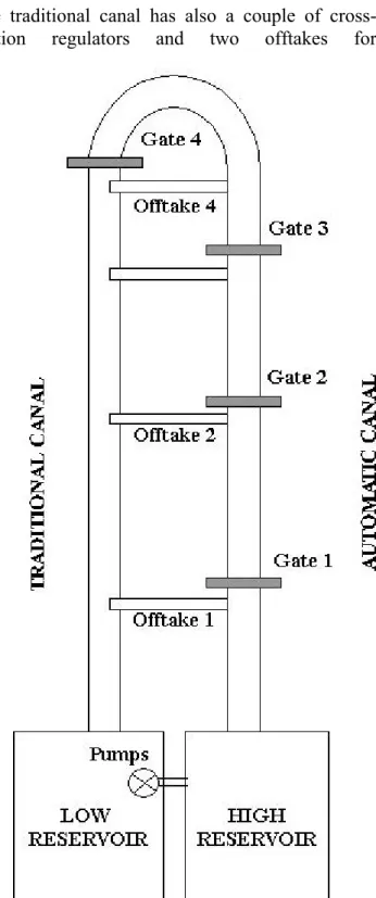
Figure 2: Schematic longitudinal representation of a generic group gate-offtake of the automatic
canal
Figure 3: Schematic representation of both traditional and automatic experimental canals each, and the geometry of its cross section is
trapezoidal (Figure 1). The hydraulic features used in project, as well as in all the following analysis, were a flow of 0,090 m3/s for a uniform water depth of 0,700 m.
The water in this experimental canal flows in closed circuit, regarding water savings; the return to the storage reservoir is guaranteed by a traditional canal.
The four pools of the automatic canal are divided by three sluice gates; the last one ends with an overshot gate, which discharges to the referred traditional canal.
Immediately upstream of each gate there is an orifice type offtake, equipped with a flowmeter, and a counterweight-float level sensor (Figure 2); a servo-motorised valve controls the flow in the offtake. The gate is also motorised and both equipments have position sensors.
The flow within the automatic canal is regulated by another servo-motorised valve located at the exit of an high reservoir (head of the automatic canal), simulating a real load situation. This high reservoir is filled with the recovered water pumped from a low one, which collects the flow from the traditional canal (Figure 3).
Regarding water savings, all offtakes discharge towards the traditional canal. Therefore, the installation has no losses of water except evaporation effects which are not, in this case, significant.
Besides these hydraulic equipments, each group gate-offtake is controlled and monitorised with PLCs responsible for all data acquisition and transfer (analogic and digital signals) as well as the control actions after appropriate programming. The traditional canal has also a couple of cross-section regulators and two offtakes for
demonstrating purposes. These equipments were not mentioned earlier because the following study will only involve automatic control chains.
It is noticeable the versatility of this experimental facilities on the field of irrigation canal studies once one can choose the length of each reach, modifying its hydraulic behaviour, as well as simulate several water demand scenarios.
3 Mathematical Modelling
The main goal of an irrigation canal is to supply water as well as transport it from its source, river or dam, for instance, to the final users, usually farmers.
3.1 Basic equations
3.1.1 Saint-Venant equations
The dynamic behaviour of these systems can be well described by a set of equations known as the Saint-Venant equations [7]: 0 = ∂ ∂ + ∂ ∂ t H B x Q (1)
(
)
0 . . 2 = − + ∂ ∂ + ∂ ∂ g A J i A Q x t Q (2) where Q is the discharge, H the water depth, B the water surface width, A the water cross-section area,g the gravity acceleration, x the longitudinal
abscissa in the direction of flow, t the time, i the bottom slope and J the energy gradient slope that can be accurately approximated by the Manning-Strickler formula: 3 4 2 2 2 R A K Q J = (3)
where K is the Manning-Strickler coefficient and R the hydraulic radius defined by R= AP, where P is the wetted perimeter.
These equations are strongly non-linear and, for real canal systems, have no known analytical solution.
3.1.2 Linearization
There are many methods to solve numerically the Saint-Venant equations in order to better study real systems. In the present case, the referred equations were in the first place made linear, to overcome their non-linearity and in order to become possible the use of linear controllers.
The equations are linearized assuming conditions near some steady state. This ensures that, for small deviations from a considered setpoint, the resulting equations will still describe the behaviour of the system.
The linearization of the Saint-Venant equations leads to ([9] cited by [3]): 0 0 ∂ = ∂ + ∂ ∂ t h B x q (4)
(
)
− ∂ ∂ − + ∂ ∂ + ∂ ∂ x h B V c x q V t q 0 2 0 2 0 0 2 0 0 0 − = −ξ q γ h (5)where q and h are the variations of discharge and water depth, respectively, from a considered steady state, c the wave celerity (c= gAB ), V flow velocity (V =QA) and 0 subscript stands for steady
state values;ξ and 0 γ are factors due to0 linearization defined by 0 0 2 0 0 3 4 0 0 2 0 0 2 2 + − = dx dH B A Q R A K gQ ξ (6)
(
)
(
)
[
co co co Fr a]
giB 2 0 0 = 1+ − 1+ + −2 γ (7) I dx dH a 0 = (8) 0 0 0 3 4 1 + = dH dR B P co (9)where Fr is the Froude number defined byFr=Vc.
In spite of having now all the necessary equations linearized, there are still many steady state parameters left to determine, exception made to
steady state discharge that one can choose freely as it is the condition for linearization.
Steady state parameters can be calculated by taking again the Saint-Venant equations and assuming no variations in discharge and flow depth in time. So, solving them leads to [7]:
2 1 Fr i J dx dH − − = (10)
This equation represents the spatial gradually varied flow and will be used to determine the flow profile in steady state flow conditions. Nevertheless, it is necessary to solve it by a numerical method, once it has no analytical solutions. As mentioned before, the values assumed are the project nominal features of the canal, i.e., discharge of 0,090 m3/s and 0,070 m of water depth.
3.1.3 Finite differences method
Although the equations are linearized, they are still partial differential equations. Thereby, by using the finite differences method they are transformed in a set of ordinary differential equations which is achieved by discretizing the equations (4) and (5). In the present study, central differences in space were chosen for the discretization:
1 1 1 1 − + − + − − = ∂ ∂ x x i i i x x M M x M (11) Applying this to the linearized Saint-Venant equations and assuming that the spaced grid is regular leads to:
x q q B t h i i i i ∆ 2 1 1 1 0 − + − − = ∂ ∂ (12)
(
)
+ ∆ − − − ∆ − − = ∂ ∂ + − + − x h h B V c x q q V t q i i i i i i i 2 1 1 0 2 0 2 0 1 1 0 i i i iq 0 h 0 γ ξ + + (13) where ∆x=xi+1−xi.As the method considered is the central differences method, it is not possible to apply it to upstream neither to downstream boundaries once there is in both cases one node that is missing.
Therefore, instead of central differences it is possible to apply forward and backward differences to downstream and upstream boundaries, respectively. x q q B t h ∆ 1 2 1 0 1 =− 1 − ∂ ∂ (14) x q q B t h n n n n ∆ 1 0 1 − − − = ∂ ∂ (15) There is no need of any equations for q1 or qn as
they are external boundary conditions.
It is known that this operation leads to a set of 2n-2 equations, if n is the number of nodes used in discretizing. So, a state space representation will be so much helpful as convenient in analysing the system from now on, once the system state is perfectly described by all these variables – state variables. Nevertheless, all further analysis will be made in frequency domain.
The form of the state space representation can be written as [4] Bu Ax x dt d + = (16) Cx y= (17)
where x is the state vector, A the state matrix, B the input matrix, y the output vector and C the output matrix.
In the present situation, it can be seen that the state vector, x, will contain the flow and depth variations in all the nodes while the input vector, u, will contain the discharges at the upstream and downstream boundaries; the output matrix will only have one non-zero element depending on which level is measured and, in this particular case, desirable of controlling. This feature it is typical of canal control, where the measured and controlled variable are the same [7].
4 Control Strategy and Numerical
Simulations
The most commonly used controller in standard applications is PID control and hydraulic systems like irrigation canals make no exception.
In general, the PID control algorithm can be written as [4]:
( )
=( )
+ e( )
t +K∫
e( )
t dt dt d K t e K t u p D I (18)where u(t) is the control action, e(t) the deviation of the controlled variable from the desired setpoint and KP, KD and KI are the proportional, derivative
and integral gains, respectively.
In most cases, the controller is reduced to a PI due to difficulties in tuning properly the derivative gain, KD ([1] cited by [2]).
Many standard ways have been developed to tune a PI controller, as the well-known and widely used Ziegler-Nichols method [4]; these empirical rules allow to determine the proportional and integral gains based on the transient response of the real system.
Transposing the problem to an irrigation canal with multiple pools and gates, it is easy to verify that any experiments who aim to determine experimentally these parameters will not be much accurate due to the interactions between the various pools of the whole canal.
The strategy adopted in the present study to determine the proportional and integral gains was to compare the frequency response of the state space model, which relies on the linearized Saint-Venant equations, with a simple model with the assumption of each pool as a reservoir (reservoir model)
So, assuming each pool as a reservoir, water depth and flow are related by
Q A H dt d Sup ∆ 1 = (19)
where H is the water depth, Q the discharge and
ASup is the superficial area of the pool.
Taking the Laplace transform to equation (19) leads to
(
in out)
Sup Q Q sA H = 1 − (20)where s is the Laplace variable.
Qin and Qout can be thought as the upstream and
downstream discharges for the considered pool of the canal for better understanding of this procedure. Taking the Laplace transform, it is possible to rewrite the equation (18), assuming no derivative gain,
( )
e( )
s s K K s u I P + = (21)Considering the water depth as the controlled variable and the discharges as control actions, equation (21) yields
(
H H)
s K K Q I ref P out − + = (22)for upstream water depth control. Combining equations (20) and (22)
− + + + = ref Sup I Sup P Sup I Sup P H A K s A K s A K s A K H 2 in Sup I Sup P Q A K s A K s s + + − 2 (23)
assuming already that both gains are negative. Equation (22) is a second order transfer function which has a global form defined by [4]
( )
2 2 2 2 n n n s s G ω ξ ω ω + + = (24)where ϖ is the natural frequency of the systemn and ξ the damping ratio.
Combining equations (23) and (24) leads to quite simple expressions for KP and KI.
A
KP =−2ωnξ (25)
A
Figure 4: Bode representations for the first pool of the canal and for both reservoir and finite
differences models
The value of ω adopted will depend of the Boden response of both systems, i.e., the selected value for calculations has to correspond to a frequency where both systems have similar behaviours.
The frequency value will be related with the lowest resonance frequency of the system by
n
r n
ω
ω = (27)
where n is an integer number that is chosen according to the condition mentioned above. In all calculations, ξ will be assumed as 1, as it is the value that better fits experimentally to this canal.
4.2 Numerical results
The Bode plot for the first pool of the canal (Figure 4) shows clearly that both models respond approximately until a certain value of frequency; any controller that will be designed must take that fact in consideration. All these plots were
computed for the first pool of the canal with all its specific geometric characteristics and assuming the transfer function n n Q H ∂ ∂ .
Now, it is possible to identify the value of the frequency of the lowest resonance peak as well as the value where the differences of both models become significant (Figure 5).
It can be seen by analysing the Bode plot above that any value of n (equation (27)) has to be greater or equal than 4. So, the values of n chosen and the correspondent proportional and integral gains calculated by equations (25) and (26) are shown in Table 1.
These values of KP and KI were submitted to
experimental testing of its performance with results and discussion shown in the following sections.
Table 1: Chosen values of n and resulting proportional and integral gains, KP and KI
Controller n KP KI A 4 -1,2 -0,024 B 6 -0,8 -0,010 C 8 -0,6 -0,006
5 Experimental Validation
5.1 Test basisAlthough in upstream control canals the main goal of any kind of regulator or control systems is to keep constant the water depth in order to provide previously accorded discharges without any significant delay, the tests here presented were not made using any offtake. These tests only intend to prove the capability of the controller with the parameters calculated by the proceeding above described.
All the tests were made only working with the first gate, having all the others controlling as well the upstream water depth in their pools, using controller C, once these had their performance already proven [8].
As mentioned before, the project nominal features of the experimental canal are a 0,090 m3/s flow and Figure 5: Bode magnitude representations of
the lowest resonance peak frequency and highest frequency value of similar behaviour of
a 0,070 m uniform water depth. So, the setpoint in water depth used in all testing was precisely 0,700 m, having the flow varying from 0,020 m3/s to a maximum of 0,080 m3/s and the other way down. The maximum project flow was not achieved because a 0,090 m3/s value was found to be quite severe for the installed equipments. Nevertheless, there are three distinct scenarios: the flow was modified in steps of 0,010 m3/s, correspondent to 11 % of the canal global capacity, 0,020 m3/s (22 %) and 0,030 m3/s (33 %).
In spite of testing had not included any offtake operations, the results can easily be thought as so, because the final selected controller will prove its capability of bringing the water level back to the desired setpoint, independently of the disturbance epicentre, flow or offtake opening. In other words, the controller will be capable of responding properly to all upstream disturbances.
5.2 Test results
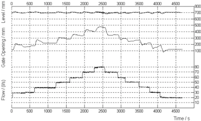
The following figures show the results of all the tests described above. An exception occurs with the
0,030 m3/s step of the controller A test, which is not presented, due to the fact of the gate opens completely as a result of the 33 % disturbance, not showing any influence on the water level.
As one can see, the controller A has a bit severe behaviour to the actuators, although it can actually accomplish the task of keeping the water level on the desired setpoint (Figures 6 and 7). This
Figure 6 – Test result of discharge step disturbances of 0,010 m3/s for the controller A
Figure 7– Test result of discharge step disturbances of 0,020 m3/s for the controller A
Figure 8– Test result of discharge step disturbances of 0,010 m3/s for the controller B
Figure 10 – Test result of discharge step disturbances of 0,030 m3/s for the controller B
Figure 9 – Test result of discharge step disturbances of 0,020 m3/s for the controller B
Figure 14 – Superposition of step disturbances of 0,010 m3/s test for the controllers B and C
Figure 15 – Superposition of step disturbances of 0,020 m3/s test for the controllers B and C performance is altered when the disturbance is 33
% of the canal capacity; in this case, the controller does not respond to the expected.
By the other hand, the controller B responds quite good to disturbances of 11 % and 22 % global capacity (Figure 8 and 9). For the last test of this controller, shown in Figure 10, the behaviour of the actuators almost reaches the similar test of the controller A, with the gate higher than the water level for a short period of time
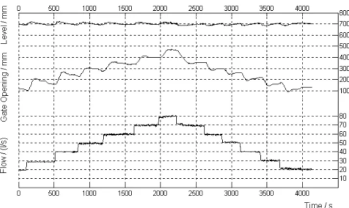
Controller C responds very well to all tests made, bringing the water level to the desired setpoint, with no significant overshoot or severe behaviour to the actuators.
Anyway, for better understanding, it is possible to zoom and superpose both controller B and C responses to 11% and 22% disturbances; 33% disturbance is not considered as it quite exaggerated disturbance to a canal of this kind (Figures 14 and 15).
In Figure 14 the differences between the controllers are not very visible due to noise measurements, although it is noticeable that controller C can bring the level back to the setpoint quicker, especially when working with higher values of flow. The differences can be better observed in Figure 15, where it becomes clear that controller C has a smaller overshoot.
Figure 11 – Test result of discharge step disturbances of 0,010 m3/s for the controller C
Figure 12 – Test result of discharge step disturbances of 0,020 m3/s for the controller C
Figure 13 – Test result of discharge step disturbances of 0,030 m3/s for the controller C
6 Discussions and Conclusions
The main objective of this paper it was to study upstream water level control in an experimental irrigation canal and design and tune a PI controller. It is clear that the goal was achieved and this technique proved its capability of properly tune the desired controller. In spite of having the advantage of using experimentally the considered canal, this can work as well as a disadvantage because not always is possible to study experimentally an irrigation canal.
By the results shown, the conclusions point that controller C must be selected for a more accurate control once it fits well the purpose of keeping the water level constant, reacting to the provoked upstream disturbances, without significant overshoot or even severe behaviour to the actuators.
Nevertheless, it was expected that the other two controllers should in fact work even better, fulfilling their goal. The reason why this was not observed, is that servo-gates have constant speed, roughly 3,75 mm/s, and for that every control actions are limited by rising and falling slew rates. Further investigation will improve these and develop another control strategies.
Acknowledgements
The study has been performed and partially financed under the research contract SIDReg-98.01.02.00002 of the INTERREG II-C Program.
References
[1] K. J. Astrom and T. Hagglung. “PID Controllers: theory, design and tuning”, 2nd Edition, Instrument Society of America, Research Triangle Park, North Carolina (1995).
[2] J.-P. Baume, P.-O. Malaterre, J. Sau. “Tuning Of PI Controllers for an Irrigation Canal using Optimization Tools”, Modernization of Irrigation
Water Delivery Systems, (Proceedings of the
USCID Workshop, Phoenix), USCID, p. 483-500 (1999).
[3] A. Hof. “Controller Design For Water Management Systems”, TU Delft (1996).
[4] B. C. Kuo. “Automatic Control Systems”, 7th Edition, Prentice Hall International Editions (1995).
[5] Matlab User’s Guide, (2000).
[6] M. Rijo. “SCADA of an Upstream Controlled Irrigation Canal System”, Modernization of
Irrigation Water Delivery Systems, (Proceedings of
the USCID Workshop, Phoenix), USCID, p. 123-136, (1999).
[7] M. Rijo, A. B. Almeida, L. S. Pereira. “Mathematical Modelling and Field Study of Unsteady Flow in an Irrigation Canal System”,
Fluid Flow Modelling, (Proceedings Of
HYDROSOFT ’92, Valencia, Spain), Computation Mechanics Publications and Elsevier Applied Science, London, p. 339-349, (1992).
[8] M. Rijo et al.. “Experimental Water Irrigation Delivery Canal, in order to study Control Strategies and to define Water Management Models in Water Shortage Situations (in Portuguese)”, Final Report
of the Research Project INTERREG II-C (Code SIDReg-98.01.02.00002) (2001).
[9] J. Schuurmans. “Control of Water Levels In Open Channels”, Ph.D thesis, 223 p., ISBN 90-9010995-1 Delft, Netherlands, (1997).