Conservation
genetics and
demography of
the hirola antelope
relict: an entire
mammal genus on
the brink of
extinction
Rui Filipe Resende Pinto
Master’s Degree in Biodiversity, Genetics and Evolution
CIBIO-InBIO (Research Center in Biodiversity and Genetic Resources)Department of Biology
2018
Supervisor
Michael J. Jowers, Post-Doctoral Researcher, CIBIO-InBIO
Co-supervisors
Raquel Godinho, Principal Researcher, CIBIO-InBIO João Queirós, Post-Doctoral Researcher, CIBIO-InBIO
Todas as correções determinadas pelo júri, e só essas, foram efetuadas. O Presidente do Júri,
Acknowledgements
I would first like to thank my supervisors Michael Jowers, João Queirós and Raquel Godinho for letting me participate in such a unique project, for their precious help, for always having an eye for detail and for the motivation they provided.
Thanks to Samer Angelone, Dr. Abdullah H. Ali (Director of the Hirola Conservation Programme), Mathew Mutinda (KWS- Field Veterinary Officer), Dr. Francis Gakuya (KWS Head of Veterinary Services), Moses Otiende (KWS), Isaac Lekolool (KWS) and everybody at the Kenya Wildlife Service for their collaboration, providing us with samples and information about hirola. Thanks to Daniel Klingberg Johansson of University of Copenhagen Zoological Museum for providing us with a museum sample.
Thanks to Paulo Célio for his support of the project, to José Carlos Brito for his help with the maps and to Rita Rocha for her advice on the analyses.Thanks to Susana Lopes, Diana Castro, Patrícia Ribeiro, Sofia Mourão, and everyone at CTM and CIBIO-InBIO, without whom this project would not have been possible.
A big thank you, Rute, for always being there for me with love and support, and sometimes a much needed cup of coffee.
My heartfelt thanks to my mother, for always having the patience and time to help me.
My sincere thanks to all the friends that walked this path with me for all their support
This work was supported by Norte Portugal Regional Operational Programme (NORTE2020), under the PORTUGAL 2020 Partership Agreement, through the European Regional Development Fund (ERDF)(NORTE-01-0145-FEDER-000007 to Nuno Ferrand).
Resumo
O hirola (Beatragus Hunteri) é considerado o antílope mais ameaçado do mundo. A sua extinção constituiria o primeiro desaparecimento de um género de mamíferos desde o tigre-da-tasmânia (Thylacinus cynocephalus) em 1936. Devido à perda de habitat e epidemias de peste bovina, entre outros fatores, os hirola sofreram um grave declínio no fim do século XX. A translocação recente para um santuário livre de predadores em 2012 criou alguma esperança para a conservação desta espécie. No entanto, o número de indivíduos existente sugere que a sua diversidade genética é reduzida devido a um possível efeito de bottleneck. Logo, um estudo genético dos hirola é necessário para futuras decisões relativas à conservação da espécie e para avaliar a existência de subestruturação genética entre grupos de vários locais para futuros programas de translocação e reintrodução. Neste estudo, foi obtida informação genética de 54 indivíduos (de uma população com menos de 500 indivíduos), através da recolha de fezes e amostras de sangue em vários locais na distribuição natural da espécie. Foi ainda obtida informação genética de uma amostra de tecido existente no museu Zoológico de Copenhaga. Um conjunto de 14 microssatélites autossómicos e a região de controlo mitocondrial completa foram utilizados para avaliar a diversidade e a subestruturação genética desta espécie, assim como a influência da história demográfica recente nos padrões genéticos.
A diversidade genética detetada (He = 0.551) foi moderada, contrastando com o número reduzido de indivíduos e recente declínio da espécie. No entanto, as sequências mitocondriais analisadas demonstraram um número diminuto de haplótipos, assim como uma diversidade nucleotídica e diferenciação haplotípica muito reduzidas. No santuário, os níveis de diversidade demonstraram ser semelhantes aos dos restantes locais. O nível reduzido de diferenciação sugere uma alta dispersão dos hirola pelo território natural, pelo menos até recentemente. Apesar de terem sido detectados sinais de um efeito de bottleneck, não foram encontradas evidências de consanguinidade populacional.
Devido ao número reduzido de indivíduos restantes e evidências que indicam que a queda populacional desta espécie criou um efeito de bottleneck genético, é aconselhável desenvolver estratégias para evitar erosão genética de modo a ser possível recuperar o número de hirolas para níveis historicamente registados.
Palavras-chave: Hirola, Antílope, Espécie ameaçada, Genética populacional, Genética da conservação, Diversidade genética, Estruturação populacional, Efeito de Bottleneck, Isolamento por distância.
Abstract
The hirola (Beatragus hunteri) is considered the most endangered antelope in the world. Its extinction would constitute the first disappearance of a mammalian genus since the Tasmanian tiger (Thylacinus cynocephalus) in 1936. Tree encroachment and a rinderpest outbreak that occurred in the 1980s, among other factors, have caused a severe decline in this species in the late 20th century. Recent translocation of wild herds to a new predator-proof sanctuary in 2012 has brought some hope to the conservation of this species. Nevertheless, the critically low population numbers of this species suggest that its genetic richness is low as a consequence of a possible bottleneck effect. Therefore, a genetic study of the hirola was in need for future conservation decisions on the species and to assess possible substructure in different locations for future translocation programmes. In the present study, genetic data from 54 individuals (from less than 500 remaining) was obtained from faeces and blood samples collected across several localities in the natural distribution range of the species in Kenya. Additionally, one museum sample was obtained from the Zoological Museum of Copenhagen. A set of 14 microsatellite loci and the complete mitochondrial control region were used to estimate genetic diversity and population structure, as well as to infer genetic imprint of recent demographic history of the species.
Patterns of nuclear genetic diversity were moderate (He=0.551), contrasting with the low numbers and recent decline of this species. However, the mitochondrial sequences obtained showed low nucleotide diversity, few haplotypes and low haplotypic differentiation. In the sanctuary, the levels of nuclear and mitochondrial diversity are similar to those in the wild. The low degree of differentiation inferred together with no evidence of population structure suggests dispersal of hirola across the natural distribution range, at least until recent times. Although signals of a genetic bottleneck were found, no inbreeding was detected.
Due to the species’ low population numbers and evidence of a genetic bottleneck caused by the recent crash, it is advisable to develop strategies to avoid genetic erosion in order to recover the number of hirolas to historical levels.
Keywords: Hirola, Antelope, Endangered species, Population genetics, Conservation genetics, Genetic diversity, Population structure, Bottleneck, Isolation-by-distance.
Table of Contents
Acknowledgements ... v
Resumo ... vi
Abstract ... vii
Table of Contents ... viii
List of Tables ... xi
List of Figures ... xiii
List of Abbreviations ... xvi
1. Introduction ... 18
1.1. The 6th extinction ... 18
1.2. Hirola, the rarest antelope ... 18
1.2.1. Lessons from the past ... 19
1.2.2. Taxonomy and etymology ... 19
1.2.3. Species description ... 20 1.2.4. Habitat ... 21 1.2.5. Social organization ... 21 1.2.6. Interspecific interactions ... 22 1.2.7. Distribution ... 22 1.2.8. Decline ... 24 1.2.9. Conservation efforts ... 24 1.2.9.1. Tsavo population ... 24 1.2.9.2. Ishaqbini conservancy ... 25 1.2.9.3. Other conservancies ... 26
1.3. Genetic diversity and conservation ... 26
1.4. Non-invasive sampling ... 27
1.5. Molecular tools to assess genetic diversity ... 27
1.5.2. Mitochondrial markers ... 28
1.6. The genetic consequences of bottlenecks ... 29
1.7. Inbreeding depression ... 30
1.8. Why genetics matter in translocations... 32
1.9. Objectives ... 33
2. Material and Methods ... 35
2.1. Study area and sampling ... 35
2.2. DNA extraction and amplification ... 36
2.3. Amplification of mitochondrial DNA control region... 37
2.4. Amplification of microsatellite markers from invasive samples ... 38
2.5. Amplification of microsatellite markers from non-invasive samples and museum sample ... 39
2.6. Data analysis ... 40
2.6.1. Probability of identity ... 40
2.6.2. Nuclear and mitochondrial genetic diversity ... 40
2.6.3. Population differentiation and structure ... 41
2.6.4. Demographic history ... 43
3. Results ... 45
3.1. Microsatellite loci ... 45
3.1.1. Genotyping, quality control procedures, and identification of repeated genotypes ... 45
3.1.2. Genetic Diversity ... 47
3.1.3. Population differentiation and structure ... 48
3.1.4. Demographic history ... 54
3.2. Mitochondrial DNA ... 54
3.2.1. Genetic diversity ... 54
3.2.2. Population differentiation and structure ... 56
3.2.3. Demographic history ... 59
3.2.4. Census population size estimation using non-invasive samples ... 61
4. Discussion ... 62
4.1. Patterns of genetic diversity in Hirola ... 62
4.3. Demographic history ... 65
4.4. Ecological factors and conservation implications ... 67
4.5. Limitations in this study and considerations for further research ... 68
5. Concluding remarks ... 70
6. Glossary ... 71
7. References ... 72
List of Tables
Table 1- Description of primers and PCR conditions used to amplify the CR1 and CR2 fragments of the mitochondrial DNA control region. ... 37
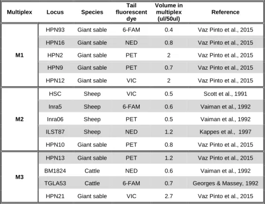
Table 2- Microsatellite markers amplified for non-invasive samples and respective information regarding the fluorescent dye used, the volume used in the multiplex and the source. This panel of markers was used for the further population genetics
analyses. ... 40
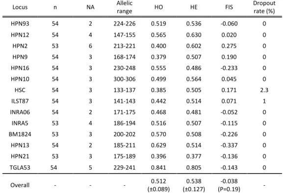
Table 3- Summary diversity statistics for the 14 autosomal microsatellite tested: n - sample size; NA - total number of alleles; HO - observed heterozygosity; HE -
expected heterozygosity; FIS - inbreeding coefficient) and allele dropout rate. ... 46
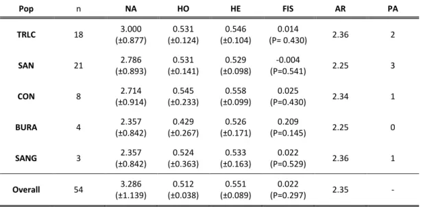
Table 4- Genetic diversity measures for each population and for the overall dataset for 14 autosomal loci: n - sample size; NA - number of alleles; H0 - observed
heterozygosity; HE - expected heterozygosity; FIS - inbreeding coefficient; AR - allelic richness; PA - number of private alleles. TRLC = Translocated population; SAN = Sanctuary population; CON = conservancy population; BURA = Bura population; SANG = Sangailu population. ... 47
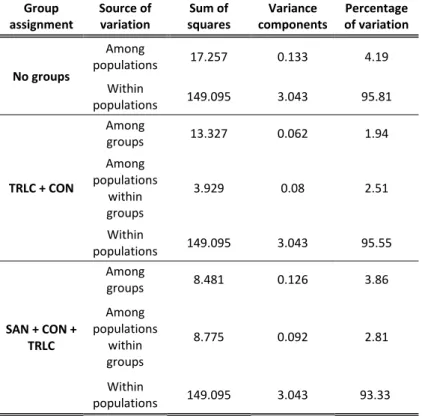
Table 5- Results of hierarchical AMOVA. The p-value is determined through the frequency of more extreme variance components than observed obtained randomly after 10,000 permutations. TRLC = Translocated; SAN = Sanctuary; CON =
Conservancy; BURA = Bura; SANG = Sangailu. ... 49
Table 6 - Queller’s and Goodnight (QG) estimator of individual relatedness for each population in averages. The minimum and maximum values are also displayed. TRLC = Translocated; SAN = Sanctuary; CON = Conservancy; BURA = Bura; SANG=
Sangailu. ... 53
Table 7- Genetic diversity statistics from the mtDNA control region: n - number of sequences; NH - number of haplotypes; HD - haplotype diversity and its standard deviation; S - polymorphic sites; π - nucleotide diversity and its standard deviation. TRLC = Translocated; SAN = Sanctuary; CON = Conservancy; BURA = Bura; SANG = Sangailu. ... 55
Table 8- Results of the hierarchical AMOVA conducted for the mtDNA control region sequences. The p-value is determined through the frequency of more extreme variance components obtained randomly after 10,000 permutations. TRLC = Translocated; SAN = Sanctuary; CON = Conservancy; BURA = Bura; SANG = Sangailu. ... 57
Table 9 - Results of neutrality tests: Tajima's D, Fu's F, Fu and Li's D and F, R2. n is the sample size, NH is the number of haplotypes and NS means non-significant result. TRLC = Translocated; SAN = Sanctuary; CON = Conservancy; BURA = Bura; SANG = Sangailu. ... 59
Table 10 - Census population size estimated using the mark-recapture models implemented in Capwire. The number of individuals estimated from equal-capture model (ECM) and two-innate-rates model (TIRM) are shown, together with the results excluding individuals with a higher number of recaptures (Partitioned) and confidence intervals for both models. ... 61
Table S1 Microsatellite markers used and tested for hirola’s invasive samples. Details of the multiplex reactions are provided. NA means no-amplification of markers. ... 92
Table S2- Details of the multiplex PCR performed for amplification of invasive samples: Species, temperature of each step (temp), time of each step (‘ denotes minutes, ‘’ denotes seconds ) and number of repeats of each denaturation, annealing and extension cycle (Nº of cycles). Negative temperatures between brackets (e.g. -0.5ºC) signifies the decrease in annealing temperature in each cycle. ... 95
Table S3- Details of the Multiplex PCR for the amplification of the museum and non-invasive samples: Temperature of each step (Temp), time of each step (‘ denotes minutes, ‘’ denotes seconds) and number of repeats of each denaturation, annealing and extension cycle (Nº of cycles). Negative temperatures between brackets (e.g. -0.5ºC) signifies the decrease in annealing temperature in each cycle. ... 97
Table S4- Maximum distance between samples of the same individual. ... 99
Table S5- Values of pairwise fixation index (FST) between populations using the microsatellite dataset on the bottom left and FST values between populations obtained using the mtDNA sequences on the top right. The single significant values is marked with an asterisk (p > 0.05). ... 99
List of Figures
Fig. 1- Hirola (Beatragus hunteri) Credit: Kenneth Coe, member of the Advisory
Council of the Nature Conservancy’s Africa Program (image displayed on the cover) 18
Fig. 2- Tasmanian Tiger at Hobart Zoo in 1933. Credit: National Archives of Australia ... 19
Fig. 3 - Comparison of phylogenetic trees obtained from the molecular analysis using complete mitochondrial genomes versus chromosomal characters. The Bayesian inference (left) showed maximum likelihood bootstrap values and posterior probabilities for each node, whereas the maximum parsimony tree (right) showed just maximum parsimony bootstrap values. The dotted line indicates the phylogenetic position of Beatragus hunteri (in bold) in both topologies. Image and caption credit: Steiner et al. (2014) ... 20
Fig. 4- a) Historical natural distribution range of hirola. Blue line and the number 2 (in the original map) indicate the location of Tsavo East National Park where there is currently an ex situ population of hirola (see section 1.2.9.1). Source: Hirola Evaluation Report (Butynski, 2000) b) Current natural distribution range (light grey) of hirola. Source: Hirola Evaluation Report (Butynski, 2000). ... 23
Fig. 5- Study area and sampling: (a) The location (marked with a square) of the sampling area in Kenya, in East Africa, and neighbouring countries; (b) Map showing the current distribution of hirola (source: IUCN, 2017): the Tsavo population (dark blue) and the natural range (yellow), where the sampling occurred; (c) Map showing the location on which sampling of hirola scats took place (Sanctuary, Conservancy, Bura, Sangailu) and of the capture sites used for the 2012 translocation (into the sanctuary). ... 36
Fig. 6- Cumulative probability of identity (PI) and probability of identity between siblings (PIsibs). ... 46
Fig. 7- Neighbor-Joining tree constructed through pairwise FST obtained for the five comparison populations using the 14 microsatellite markers. Only one FST value was
found, between TRLC and BURA. TRLC = Translocated; SAN = Sanctuary; CON = Conservancy; BURA = Bura; SANG = Sangailu. ... 48
Fig. 8- Factorial correspondence analysis performed in GENETIX using the 14
microsatellite markers. TRLC = Translocated; SAN = Sanctuary; CON = Conservancy; BURA = Bura; SANG = Sangailu. ... 50
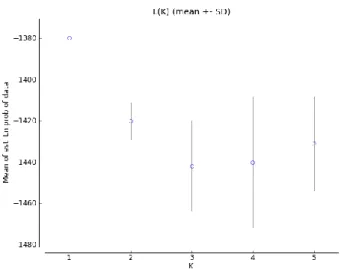
Fig. 9- Inference of the most probable number of clusters (K) using the mean of estimated Ln probability of data, obtained in STRUCTURE HARVESTER. K=1 was chosen as the best solution. ... 50
Fig. 10- Bar plot obtained in STRUCTURE for K=2 and K=3 ... 51
Fig. 11- Map of cluster membership for the run with highest average posterior
probability (K=4). X and Y graph correspond to UTM coordinates. ... 52
Fig. 12- Mantel test performed using microsatellite data to test the hypothesis of isolation by distance (R = Pearson correlation coefficient; P = P value). This graph shows the relationship between genetic distance and geographic distance. ... 52
Fig. 13- Mantel test performed between populations, using microsatellite data to test the hypothesis of isolation by distance (R = Pearson correlation coefficient; P = P value). This graph shows the relationship between genetic distance and geographic distance. ... 53
Fig. 14- Plotting of frequency distribution of allele classes for microsatellite markers. Figures along the x-axis represent classes of frequency of alleles (e.g. 0.0 represents alleles with frequency lower than 0.1) and figures along the y-axis represent the proportion of alleles in those classes. A non-shifted, or L-shaped, distribution was revealed as the low-frequency class (0.0) has more alleles than any of the other
classes... 54
Fig. 15- Neighbor-Joining tree constructed through pairwise FST obtained for the five comparison populations using the mtDNA control region sequences. No FST values were considered statistically significant. TRLC = Translocated; SAN = Sanctuary; CON = Conservancy; BURA = Bura; SANG = Sangailu. ... 56
Fig. 16- Median-joining network based on mtDNA control region sequences.
Populations are distinguished through different colours and node size is dependent on frequency of sequences. Each mutation is represented by a hatch mark. Table
demonstrating the number of individual per haplotype and population. Note that Genbank and museum sequences were included in this analysis. TRLC = Translocated; SAN = Sanctuary; CON = Conservancy; BURA = Bura; SANG=
Sangailu. ... 58
Fig. 17 - Mitochondrial DNA Mantel test of isolation-by-distance. This graph shows the relationship between genetic distance and geographic distance. ... 58
Fig. 18 - Mismatch distribution analysis with observed distribution, represented by a dotted line, and expected distribution, represented by a black line, under a model of constant population size. ... 60
Fig. 19 - Bayesian skyline plots constructed in BEAST. The Y axis indicates population size and the X axis represents time (in years) from present to past. The solid line represents the median estimate and the blue area shows a 95% confidence interval. 60
Fig. S1- Permit letter by Dr. Francis Gakuya, Head of Veterinary Services of Kenya Wildlife Service (KWS). ... 91
Fig. S2- Map of duplicate samples of individuals (Ind) in the sanctuary and in the conservancy (Ind 24). Same color represents the same individual. ... 98
Fig. S3- Map of duplicate samples of individuals (Ind) in Bura East. Same color
represents the same individual. ... 98
Fig. S4- Map of cluster membership obtained in GENELAND run with second highest average posterior probability under the correlated allele frequency model X and Y graph correspond to UTM coordinates. ... 100
Fig. S5- Map of cluster membership obtained in GENELAND run with highest average posterior probability under the uncorrelated allele frequency model. X and Y graph correspond to UTM coordinates. ... 100
Fig. S6- Map of cluster membership obtained in GENELAND run with third highest average posterior probability under the correlated allele frequency model. X and Y graph correspond to UTM coordinates. ... 101
Fig. S7- Distribution of hirola observed during aerial survey performed in 2011. Credit: King et al. (2011) ... 102
List of Abbreviations
AMOVA – Hierarchical analysis of molecular significance AR – Allelic richness
BSP – Bayesian Skyline Plot CON – Conservancy
CR1 – first fragment of the control region amplified CR2 – second fragment of the control region amplified dNTPs – deoxyribonucleotide triphosphates
ECM – Equal-capture model ESS – Effective sample size FC – Factorial component
FCA – Factorial correspondence analysis FIS – Inbreeding coefficient
FST – Fixation index HD – Haplotype diversity HE – Expected heterozygosity HKY – Hasegawa, Kishino and Yano HO – Observed heterozygosity HWE – Hardy-Weinberg equilibrium
ISAG – International Society for Animal Genetics IUCN – International Union for Conservation of Nature K – Number of genetic clusters
LD – Linkage disequilibrium LRT – Likelihood ratio test
MCMC – Monte Carlo Markov chain mtDNA – Mitochondrial DNA
NA – Number of alleles
NH – Number of haplotypes NJ – Neighbor-joining
NRT – Northern Rangelands Trust PA – Private alleles
PART – Partitioning
PCR – Polymerase chain reaction
PIC – Polymorphism information content pID – Probability of identity
pIDsib – Probability of identity assuming siblings QG – Queller’s and Goodnight
RFLP- Restriction fragment length polymorphism RTF - Hirola Task Force
S – Number of polymorphic sites SAN – Sanctuary
SANG – Sangailu
TIRM – Two-innate-rates model TRLC - Translocated
UTM – Universal Transverse Mercator π – Nucleotide diversity
1. Introduction
1.1. The 6th extinction
The world is losing species at an alarming rate: up to 100 times faster than the natural “background” rate (Ceballos et al., 2015). Some scholars are even calling it an anthropogenic sixth mass extinction (Ceballos et al., 2015). This loss of biodiversity is one of the most critical environmental problems today and it is estimated that 25% of all mammals are threatened (IUCN, 2014) due to deterministic (habitat loss, over exploitation, introduced species and pollution) and stochastic (demographic, environmental, genetic and catastrophic) factors (Shaffer, 1981). Even in species that are not currently endangered, the loss of populations is frequent and widespread, at a much higher rate than natural species-level extinctions, having profound negative impacts on ecosystem diversity (Hughes et al., 1997; Ceballos & Ehrlich, 2002).
1.2. Hirola, the rarest antelope
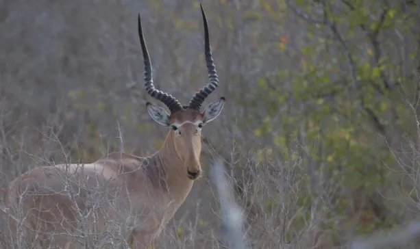
The hirola (Fig. 1), or Hunter’s antelope (Beatragus hunter; Sclater, 1889), also known as Hunter’s hartebeest, is the rarest antelope in the world and is endemic to north-east Kenya and south-west Somalia (where it may already be extinct; see Fig. 4; IUCN, 2017).
Fig. 1- Hirola (Beatragus hunteri) Credit: Kenneth Coe, member of the Advisory Council of the Nature Conservancy’s Africa Program (image displayed on the cover)
Its population decreased from around 14,000 in the 1970s to less than 500 individuals today, although some estimates are even lower, and the hirola is now considered critically endangered by the IUCN Red List of Threatened Species (IUCN, 2017).
1.2.1. Lessons from the past
The loss of the hirola can be compared with that of the Tasmanian tiger (Thylacinus cynocephalus) in 1936. This marsupial carnivore, the largest one in modern times, was unique as it was the last species of its family (Thylacinidae; Prowse et al., 2013). When attacks on sheeps in Tasmania started to be credited to this species, bounties on the Tasmanian tiger led to its intensive hunting; this, combined with disease, introduction of dogs and human intrusion in its habitat, led to the decline and eventual extinction of this iconic species (Prowse et al., 2013). Hirola’s extinction would be the first of an entire mammal genus since the extinction of the Tasmanian Tiger and, thus, the first in contemporary human history.
1.2.2. Taxonomy and etymology
The species was named and described by P. L. Sclater in 1889 as Hunter’s antelope in honor of H.C.V. Hunter, who collected the type specimen in 1887, in the eastern bank of the Tana River; the common name, hirola, is believed to be derived from the Somali name for this animal, “Aroli” (Andanje & Ottichilo, 1999; Butynski, 2000). Hirola belongs to the subfamily Alcelaphinae of the family Bovidae; its taxonomy has been controversial and its morphology has led to this species being attributed to the genus Damaliscus (as
Fig. 2- Tasmanian Tiger at Hobart Zoo in 1933. Credit: National Archives of Australia
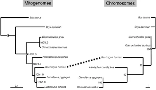
D. hunteri) or even a subspecies of the topi (as Damaliscus lunatus hunteri) before being placed in its own genus as Beatragus hunter (Andanje, 2002). Karyotypic and mithochondrial DNA analyses (Kumamoto et al., 1996; Pitra et al., 1997; Steiner et al., 2014) support the separation of hirola into its own genus (Fig.3). Male hirola exhibit the behaviour known as flehmen (a form of urine-testing to determine sexual receptivity), which is present in all bovids with the exception of Damaliscus and Alcelaphus; it has been argued that this is a strong argument in favour of the separation of hirola from Damaliscus or Alcelaphus (Estes, 1999). There are also fossil records that support this separation as these suggest that hirola is the only extant member of an older lineage than both Damaliscine and Alcelaphine antelopes (Kingdon, 1982).
1.2.3. Species description
Hirola are sometimes described as being similar to species of Damaliscus and Alcelaphus but present differences in horn and body shape and coloration (Butynski, 2000). This medium-sized antelope possesses white markings around the eyes resembling spectacles, with an inverted white chevron between the eyes, which has earned this species the nickname of “the four-eyed antelope” (Andanje, 2002; Bain, 2010). It presents a tawny or yellow-brown coloration (Butynski, 2000). Hirolas weigh between 80 and 120 kilograms and stand 1 to 1.25 meters tall at their shoulder. They present curved lyrate-shape horns, rising from the brow, coming to long, slim, sharp
Fig. 3 - Comparison of phylogenetic trees obtained from the molecular analysis using complete mitochondrial genomes versus chromosomal characters. The Bayesian inference (left) showed maximum likelihood bootstrap values and posterior probabilities for each node, whereas the maximum parsimony tree (right) showed just maximum parsimony bootstrap values. The dotted line indicates the phylogenetic position of Beatragus hunteri (in bold) in both topologies. Image and caption credit: Steiner et al. (2014)
points (Andanje, 2002).Males and females look similar although males are slightly larger with thicker horns and darker coats (Kingdon, 1982; Butynski, 2000). There is no documented evidence for morphologic variation across this species’ range.
1.2.4. Habitat
Hirola are adapted to arid environments, with an annual precipitation of 300-600 mm2, and open to lightly bushed grasslands and wooded savannahs with scattered trees and small shrubs (Bunderson, 1981). They are more dispersed during the wet season than in the dry season due to the scarcity of pasture in the latter. Hirola have been described as a grazer species (Kingdon, 1982) but browsing has been observed during the dry season (Bunderson, 1981). They prefer short, green grasses (Panicum infestum, Digitaria rivae, Latipes senegalensis and Cenchrus ciliaris) but occasionally feed on forbs (Portulaca oleraceae, Tephrosia subtriglora and Commelina erecta) (Andanje & Ottichilo, 1999).
1.2.5. Social organization
Males of this species form bachelor herds, with up to 38 individuals, and females with offspring form groups that range from 5 to 40 animals and are often accompanied by a mature male. Hirola are seasonal breeders as the mating season peaks in March at the start of the main rainy season and most calves are born at the start of the short wet season (late September, October and November), after a gestation period of around 7.5 months (Andanje, 2002). When sub-adult males leave nursery herds, at around six months of age, they may join a bachelor group of older males, a group of Grant’s gazelles (Nanger granti) or other dispersing female hirola or just stay alone (Andanje & Ottichilo, 1999). When old enough (32 months), they can form their own family herds or take the place of a male in control of a family herd (Andanje, 2002). They reach adult size at three years of age (Butynski, 2013). It is known that mature males can occupy and actively defend territories of up to 7 km2, which they mark with their preorbital scent gland,if these present good quality pasture (Andanje, 2002; Butynski, 2013). Females leave their family groups when around nine months of age and frequently join an adult male, a group of Grant’s gazelles or young males in mixed-sex yearling herds or just remain alone (Andanje, 2002). They mature at 1.5–2 years and first give birth at 2–3 years (based on records from captive animals; Butynski, 2013). Generation lenght of this species is
mentioned in the IUCN Red List as 5.4 years (IUCN, 2017) but recent estimates (Cooke et al., ) are of 6.3 years.
1.2.6. Interspecific interactions
Hirola are frequently in the company of other species, such as the above mentioned Grant’s gazelle, the Grant’s zebra (Equus quagga boehmi) (Andanje & Ottichilo, 1999), the fringe-eared oryx (Oryx callotis) (Lee et al., 2013) and the coastal topi (Damaliscus lunatus topi) (Kingdon, 1982), possibly to reduce need for vigilance and predation risk (Andanje, 2002). Hirola avoids association with kongoni (Coke’s hartebeest - Alcelaphus cokii), even though they occur in Tsavo National park (see section 1.2.9.1) alongside hirola and use similar resources, which might be indicative of competition (Andanje, 2002). Hirola also suffer from competition for good quality pasture with livestock, which has been pointed out as a factor impeding their population recovery (Andanje, 2002; Ali et al., 2017, 2018). This species’ main predators in the Garissa district are lions (Panthera leo) and African wild dogs (Lycaon pictus) (Andanje, 2002), although they can also be preyed on by cheetah (Acinonyx jubatus) and hyenas (Crocuta crocuta). Also, smaller predators like serval cat (Felis serval), caracal (Felis caracal) and black-backed Jackal (Canis mesomelas) can hunt young hirola (Kingdon, 1982; Andanje, 2002).
1.2.7. Distribution
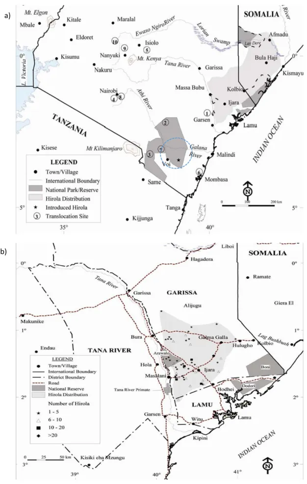
Hirola are believed to be the relict population of a lineage (Kingdon, 1982) that, based on fossil evidence, originated 3.1 million years ago and was once widespread in Eastern Africa and probably also in South Africa (Kingdon, 1982). Beatragus antiqus, hirola’s likely ancestor, was larger and had a broader skull and more upright horn cores and fossils of this extinct species were found in Tanzania, Ethiopia and Kenya, dating back to the Early Pleistocene. Fossils of B. hunteri were discovered in Tanzania, Ethiopia, Djibouti and possibly South Africa. Records of the extant species indicate that their original range lies somewhere to the south of Garissa town in Kenya, 30-50 km inland, from and parallel to the Indian Ocean, east of the Tana River, to the north of Kismayu on the west of the Juba River in Somalia (Butynski, 2000; Andanje, 2002). Bunderson (1976) estimated that hirola occupied 12,000 km2 in Kenya and 2,000 - 3,000 km2 in Somalia based on information from aerial surveys, giving a total range of 14,000-15,000
a)
Fig. 4- a) Historical natural distribution range of hirola. Blue line and the number 2 (in the original map) indicate the location of Tsavo East National Park where there is currently an ex situ population of hirola (see section 1.2.9.1). Source: Hirola Evaluation Report (Butynski, 2000) b) Current natural distribution range (light grey) of hirola. Source: Hirola Evaluation Report (Butynski, 2000).
km2, but, by 1996, their distribution in Kenya had been limited to only 42% of its original size (see Fig. 4 and Fig. 5; Butynski, 2000). Hirola is currently distributed in Kenya between Ijara, Bura and Galmagalla, over an area of around 1,200 km (Butynski, 2000). The current status on distribution range in Somalia is unknown but the former range has been affected by civil and military conflicts and it has been reported that the Somali population is probably extinct (Andanje & Ottichilo, 1999; IUCN, 2000).
1.2.8. Decline
The Kenyan population suffered a rapid decline in its numbers from around 14,000 in 1976 to less than 500 in 1995, estimated through aerial surveys (Bunderson, 1976; Ottichilo et al., 1995). The main reason for this was an outbreak of rinderpest (Morbillivirus) in the 1980s that led to mass mortality of hirola and other ruminants in Eastern Kenya although other factors like drought, poaching, predation, competition with livestock, habitat loss and degradation have also contributed to this recent decline (Butynski, 2000; Andanje, 2002; Ali et al., 2014b). Using the estimates of generation time of 6.3 for this species present in Cooke et al. (2018), the sudden decline occurred around 5 or 6 generations ago. In the Arawale National Reserve, population of hirola declined dramatically due to neglect of the reserve, which permitted the presence of poachers, livestock grazing and semi-permanent settlements (Magin, 1996; Butynski, 2000). Questions remained on why the eradication of rinderpest did not prompt the recovery of hirola in the subsequent years. Habitat loss due to tree encroachment has been pointed out as the main factor that is impeding recovery of the hirola (Ali et al., 2017).
1.2.9. Conservation efforts
1.2.9.1. Tsavo population
In 1963, a group of 30 individuals were translocated from its wild range, in Garissa district, to the Kenya’s Tsavo East National Park, which covers an area of 13,000 km2 and is situated in south-east Kenya (see Fig.4), but some perished soon after release and only less than 20 individuals remained (Andanje & Ottichilo, 1999; IUCN, 2000).
In 1996, C. Magin developed a hirola recovery plan with two main objectives: improved protection and management in the natural range and effective conservation of translocated populations in Kenya (Magin, 1996). The Hirola Task Force (RTF) was formed, composed of government organizations, NGOs and private individuals who
shared the common goal of conserving hirola in Kenya (Andanje, 2002). A study by Andanje and Ottichilo (1999) estimated a total of 76 hirola by 1995 in Tsavo. To apply Magin’s recovery plan, the RTF undertook a translocation of hirola (n = 35) in 1996 from the natural distribution range to boost the population in Tsavo East National Park (Butynski, 2000). This additional translocation was intended to enable a closer scientific study of the species and to boost the genetic composition of the Tsavo population in order to help ensure the persistence of the only ex-situ population of hirola (Andanje, 2002). However, by December 2000, the population had decreased to 77 individuals (Andanje, 2002). Analysis of the growth rate and age structure of this population indicated high calf and juvenile mortality and a low recruitment rate (Andanje & Ottichilo, 1999), which is usually due to inbreeding or decline in genetic variability (Berger, 1990). The population in Tsavo East National Park is more vulnerable to adverse genetic factors due to the low number of founder individuals than the population in the natural range (Butynski, 2000). The Tsavo population mixes and is not as territorial as wild groups (Ali, 2013; Ali et al., 2014a, 2014b), which might suggest that there is higher genetic differentiation between wild groups than in the Tsavo’s population. Genetic differentiation between and within populations is unknown.
1.2.9.2. Ishaqbini conservancy
In the year of 2005, four local communities, in collaboration with the Northern Rangelands Trust (NRT), proposed the establishment of the Ishaqbini Hirola Conservancy. This community-based conservation area, situated in the Ijara district in Garissa County, Kenya, covers around 215 km2 along the eastern bank of the Tana River. Within this conservancy, there is a predator-proof fenced sanctuary that covers 25 km2, which was established with 48 hirola in August 2012 (Ali, 2016). By the end of April 2016, the population had doubled to around 100 individuals in the sanctuary with a higher proportion of calves than in the rest of the conservancy (King et al., 2016). Herds inside the sanctuary are larger and have more calves and sub-adults than herds outside the sanctuary, suggesting less calf mortality (King et al., 2016). In the sanctuary, from its establishment in August 2012 to April 2016, only two calves died, immediately after birth, representing a 3% mortality, which contrasts with a 44% calf mortality in the conservancy (Ali et al., 2017). The calf mortality in the conservancy is similar to calf mortality in the wild (41.2%-69.8%; Andanje, 2002).
1.2.9.3. Other conservancies
There is also been an effort to increase the protected area in the hirola’s native range. Three new conservancies have been established: Bura East Conservancy (5,195 km2), Sangailu Conservancy (800 km2) and Gababa Conservancy (330 km2) (Ali, 2016). Recently, Bura East Conservancy received its registration certificate (Robb-McCord, 2017).
1.3. Genetic diversity and conservation
Biodiversity refers to the variety present in all organisms and to the interactions among them, including those they form with their abiotic environment (DeLong 1996). It is comprised of three levels which are all important to conserve. The species level is formed by the differences between species and the genetic level represents the genetic variability between conspecific individuals. At a higher level of organization, there is the ecosystem level which denotes diversity between ecosystems, and englobes habitat variation, biological communities and ecological processes (Frankham, 1995a).
The total number of genetic differences in a species or a population forms the genetic diversity. Since it was discovered, through the first population genetic studies, that species usually present a great number of polymorphisms (Harris, 1966; Lewontin & Hubby, 1966), these differences started to be considered as a requirement for biological evolution. Data from early genetic studies using allozymes and subsequent data from DNA sequencing showed that genetic diversity differs to a great extent among different species (McVean et al., 2005; Begun et al., 2007; Lack, 2015; Ellegren & Galtier, 2016). Genetic diversity increases over time as mutations occur due to DNA replication errors or mutagen-induced DNA damage (Ellegren & Galtier, 2016). The rate at which these mutations appear is variable between distinct areas of the genome (Hodgkinson & Eyre-Walker, 2011) and is also different between different species (Lynch, 2010), which might be one of the factors responsible for the high level of variation in genetic diversity (Ellegren & Galtier, 2016). The rate of allelic loss and fixation (when only one of the alleles remains) is also a determinant of genetic diversity (Ellegren & Galtier, 2016). Loci with neutral alleles are largely influenced by genetic drift (Charlesworth, 2009).
Genetic diversity is important for species to deal with changes in their environment. The current climate change, for example, has put a great pressure on species to adapt and change their behaviour (e.g. migrations) and distribution (McCarthy, 2001). Genetic diversity plays a great part in this as it determines the ability for a species to survive in a
new habitat by increasing the chance that some individuals have genetic differences. This improves their chances of surviving in unexpected conditions and, as such, improve their fitness (Sober, 1994). Another way in which genetic diversity is important for the resilience of endangered species is that these generally have small populations (Baillie et al., 2004), in which inbreeding is inevitable (Frankham et al., 2002). This causes homozygosity, which increases the chances of offspring being affected by recessive or deleterious traits (inbreeding depression; Charlesworth & Willis, 2009). In conclusion, low levels of genetic diversity increase the extinction risk by limiting potential for adaptation and by the accumulation of deleterious alleles (Reed et al., 2002). Therefore, it is pivotal to preserve genetic diversity, which has led to the field of conservation genetics (Primmer, 2009), which applies principles of population genetics to preserve the genetic diversity of species and their populations (Wayne & Morin, 2004).
1.4. Non-invasive sampling
In studies of endangered or elusive species, or in any study where disturbing the individuals of interest would be limited by ethical and practical constraints, the use of non-invasive genetic sampling is essential (Taberlet et al., 1999). There are many difficulties in amplifying DNA from non-invasive samples due to the typically low quantity and quality of existent DNA in these samples as well as to the presence of PCR inhibitors (Waits & Paetkau, 2005). However, many techniques have been developed to counteract these problems and non-invasive sampling has been widely used to study natural populations (Beja-Pereira et al., 2009; Oliveira et al., 2010; Chaves et al., 2012; Ferreira et al., 2018). Faeces are among the most widely used non-invasive samples as it is easier to find in the wild and more informative, especially when it is possible to collect them just after seeing the animals defecating (allowing to collect fresh, less degraded faeces and providing information about the species and sex of the individual; Beja-Pereira et al., 2009).
1.5. Molecular tools to assess genetic diversity
Like many fields in biology, the field of conservation genetics had its progress catalysed by technological advances, namely improvements regarding the choice of molecular markers. Studies of genetic diversity were not possible until the use of allozyme electrophoresis. This method was used to estimate the heterozygosity of allozymes (allelic variants of enzymes), which was generally assumed to reflect overall genetic
variability and, as such, it was believed it should be considered in decisions about the management of population and species (Bader, 1998).
This field had another major breakthrough with the development of DNA-based markers, which allowed to assess DNA variation itself instead of relying on variations in the electrophoretic mobility of the proteins (Schlötterer, 2004). The discovery of restriction endonucleases led to the use of restriction fragment length polymorphisms (RFLP) (Botstein et al., 1980). This concept was later applied to minisatellites and microsatellite analyses, the latter having the advantage of being smaller than the former, making it easier to amplify with polymerase chain reaction (PCR) (Schlötterer, 2004). The invention of PCR allowed, for the first time, to amplify any genomic region without isolating large amounts of clean DNA (Schlötterer, 2004).
1.5.1. Microsatellites
Microsatellites are short sections of DNA where a simple motif, generally 1-6 bp long, is repeated up to about 100 times (Richard et al., 2008). This is due to DNA replication slippage and the mismatch repair system (Schlötterer, 2000). The number of repeats of the motif varies, leading to high polymorphism levels among individuals (Bruford & Wayne, 1993). Microsatellite markers are highly polymorphic, abundant and fairly evenly distributed across eukaryotic genomes. This, coupled with their simple amplification and genotyping, even from non-invasive sources of DNA, their co-dominant nature and their typically high levels of allelic diversity at different loci, led to microsatellite markers being considered as the best molecular tools in population genetics, social structure, mating success and population movement (Schlötterer, 2000; Sunnucks, 2000), at least until the development of next-generation sequencing, which refers to new methods that reduced the cost of sequencing and produce high quality, robust data, with low noise (Buermans & den Dunnen, 2014).
1.5.2. Mitochondrial markers
In eukaryote cells, there is a comparatively small portion of DNA present in the mitochondria, known as mitochondrial DNA (mtDNA), in the form of a double-stranded, covalently closed circular molecule, with 37 coding genes, essential for normal mitochondrial function, and a control region in animals (Avise et al., 1987; Moritz, Dowling, & Brown, 1987). MtDNA is often used in population genetics and evolutionary
studies due to its lack of recombination (useful to assess clear genealogies and ancestry data), ease to isolate and assay and high mutation rate compared to nuclear DNA (Avise et al., 1987; Harrison & Quinn, 1989). It is often used to amplify DNA from non-invasive samples as it is easier to obtain from samples with low DNA quantity and quality, due to the high number of mitochondrial copies per cell (Harrison & Quinn, 1989; Waits & Paetkau, 2005). Nevertheless, it is limited by the fact that it is solely maternally inherited and, thus, may induce bias due to the fact that it is not susceptible to recombination and only reflects the female portion of the history of the species which may be different from the history of the species as a whole. The control region presents a displacement loop structure in vertebrates (D-loop), which has a function in the replication process (Moritz et al., 1987). Due to the fact that it is the most variable region of mtDNA, it is useful to assess phylogenetic relationships and intra-populational genetic diversity (Birungi & Arctander, 2000).
1.6. The genetic consequences of bottlenecks
In Africa, many large mammals have experienced severe recent population declines due to anthropogenic pressures and climatic fluctuations (Hilborn et al., 2006; Stoner et al., 2007). These population declines may lead to a great loss of genetic diversity (Groombridge et al., 2000; Weber et al., 2000; Wisely et al., 2002; Bellinger et al., 2003). This occurs because a limited number of randomly selected individuals create a founding population, leading to genetic drift. This effect is known as genetic bottleneck. A bottleneck decreases the population’s ability to adapt to and survive environmental changes, like climate change or a shift in available resources (Lande, 1988). Alternatively, if the survivors of the bottleneck are the individuals with the greatest genetic fitness, the frequency of the fitter genes within the gene pool is increased, while the pool itself is reduced. Nevertheless, the reduction in the number of individuals leads to inbreeding and, consequently, increases homozygosity, increasing the potential for inbreeding depression to occur. Smaller population size can also cause deleterious mutations to accumulate (Lynch et al., 1995). There are many species with once widespread distributions that now exist only in remnant, isolated populations in protected areas or patchy distributions, with disrupted gene flow. This population fragmentation further increases the loss of genetic diversity, constituting a serious challenge for long-term conservation (Young & Clarke, 2000; Hedrick, 2005). On the other hand, the levels of genetic diversity increase very slowly with time as random mutations accumulate or when gene flow with another population occurs. Thus, the extinction risk of bottlenecked
populations with low genetic diversity can be decreased through the introduction of individuals from other populations (Frankham, 2015; Weeks et al., 2017; Hasselgren et al., 2018)
A number of studies have shown low genetic diversity on recently bottlenecked populations of ungulates (e.g.: Armstrong et al., 2011; Godinho et al., 2012; Vaz Pinto et al., 2015). Although no genetic studies have assessed the variation in remaining hirola populations, it is suspected that remaining genetic variation is low due to the population crash and the high calf and juvenile mortality found in the Tsavo population and in the Ishaqbini population outside of the sanctuary (Andanje, 2002; Probert, 2011; Ali et al., 2014, 2018). However, in the Ishaqbini sanctuary population, calf and juvenile mortality is low and the population is increasing rapidly, showing no signs of inbreeding depression (Ali et al., 2016; King et al., 2016).
To estimate the loss of genetic diversity caused by a bottleneck, pre-bottleneck museum samples are often used as they allow a comparison between haplotypes found in current samples and haplotypes that were present before the bottlenecks (Culver et al., 2008).
1.7.
Inbreeding depression
Inbreeding depression is the decrease in fitness that results from low genetic variability, as a consequence of either increased homozygosity for deleterious recessive mutations, increased homozygosity for alleles at loci in which heterozygosity is the favoured genotype (‘overdominance’) or a combination of both. Deleterious alleles will generally be present in populations at low frequencies (mutation–selection balance), whereas overdominant alleles at a locus are maintained at intermediate frequencies by balancing selection. (Charlesworth & Willis, 2009)
Inbreeding has been proven to have a negative effect on reproduction and survival, including sperm production, mating ability, female fecundity, juvenile survival, mothering ability, age at sexual maturity and adult survival (Hedrick, 1995; Frankham et al., 2002; Johnson et al., 2010; Casas-Marce et al., 2013). Deleterious effects of inbreeding have been widely reported for wildlife in natural habitats (Keller & Waller, 2002; Dunn et al., 2011; Walling et al., 2011). There is also evidence that inbreeding depression has more impact in populations under stressful environmental factors (Miller, 1994). Nevertheless, the severity of inbreeding depression is dependent on several factors, like genetic purging (Lacy & Ballou, 1998) and the natural level of inbreeding/outbreeding of a species (Husband & Schemske, 1996; Charlesworth & Willis, 2009). In some cases,
repeated bottlenecks can lead to genetic purging diminishing the negative effects of post-bottleneck inbreeding (Amos & Harwood, 1998; Frankham, 2005). Evidence has shown that, to a certain intensity, inbreeding depression can be beneficial to the general fitness of the populations due to the effects of genetic purging, which eliminates deleterious mutations and alleles that diminish fitness; however, the effect of genetic purging seems to be modest in small populations as small deleterious effects tend to become effectively neutral and drift to extinction and empirical evidence has found only moderate effects of purging (Frankham, 2005).
As it has been shown that inbreeding reduces reproduction and survival, it is only natural that it increases extinction risk, which was first demonstrated in laboratory populations of Drosophila, houseflies and mice (Frankham, 1995b; Bijlsma et al., 1999; Bijlsma et al., 2000; Reed & Bryant, 2000; Reed et al., 2002; Reed et al., 2003), even in experiments with rates of inbreeding within the range of many endangered species (Reed & Bryant, 2000; Reed et al., 2003). Although the effect of inbreeding is harder to understand and assess in wild populations, there are studies that clearly demonstrate its contribution to extinction risk (Newman & Pilson, 1997; Saccheri et al., 1998; O’Grady et al., 2006).
Computer projections performed with conservative levels of inbreeding depression and taking into account the effects of demographic and stochastic factors and of genetic purging showed a clear negative effect of inbreeding depression on population viability across a broad taxonomic range (Brook et al., 2002; Frankham, 2005). There is the possibility that small populations are driven to extinction due to stochastic factors before low genetic diversity has an impact on the population (“Lande scenario”) (Lande, 1988). However, even though quick population decline can diminish the effects of inbreeding depression, most threatened populations are not driven to extinction before being affected by adverse genetic factors (Spielman et al., 2004).
There are small surviving populations whose fitness is apparently normal (Craig, 1994; Elgar & Clode, 2001), which has led to doubts about the negative role of inbreeding and loss of genetic diversity on population viability and extinction risk. For example, Chatham Island black robins (Petroica traversi), golden hamsters (Mesocricetus auratus) and Mauritius kestrels (Falco punctatus) all survived population bottlenecks in which only a single breeding pair remained (Groombridge et al., 2000; Frankham et al., 2002). Black-footed ferrets (Mustela nigripes) recovered from an extreme bottleneck that left them with only 18 individuals and now has more than a thousand individuals across several populations (Wisely et al., 2002), the northern elephant seal (Mirounga angustirostris)
rebounded from 20-100 individuals a century ago to 175,000 today (Weber et al., 2000) and the plains bison (Bison bison bison) were once only distributed in five small herds (Hedrick, 2009). Nevertheless, these observations are highly selective and ignore the vast majority of cases of small populations that did not avoid extinction (Frankham, 2005).
It is important to devise conservation plans to reduce inbreeding in populations of conservation interest due to its effects on fitness and on the extinction risk of small populations (Frankham, 2005; Keller et al., 2007). One way to reduce inbreeding is the crossing of unrelated populations (Spielman & Frankham, 1992; Falconer & Mackay, 1996). This method has been proven to be effective in the wild in deer mice (Peromyscus maniculatus; Schwartz & Mills, 2005), gray wolf (Canis lupus; Vilà et al., 2003), greater prairie chicken (Tymphanuchus cupido pinnatus; Westemeier et al., 1998) and adders (Vipera berus; Madsen et al., 2004).
1.8.
Why genetics matter in translocations
Although translocations have been an important tool in species conservation (IUCN, 2013), they are often unsuccessful and expensive and, as such, there is growing interest in the factors that determine their success, namely genetic ones (Fischer & Lindenmayer, 2000). There are different types of translocation (IUCN, 2013):
- Population restoration denotes “conservation translocations to within indigenous range” and is comprised of:
- Reinforcement (movement of individuals into a population of conspecifics);
- re-introduction (movement of an organism into a part of its native/historical range from which it has disappeared).
- Conservation introduction indicates “the intentional movement and release of an organism outside its indigenous range” and comprises:
-Assisted colonisation, which aims to avoid the extinction of populations of the focal species;
-Ecological replacement, which has the objective of translocating an organism to perform a certain ecological function.
Although the genetic effects of a translocation are often overlooked, there has been increasing evidence that these are crucial for population establishment and persistence
(Weeks et al., 2011). For instance, reinforcement can be used to increase the population size of a threatened species in order to alleviate the risk of stochastic loss but it can also decrease the risk of low genetic variability and, consequently, the risk of inbreeding depression (Hedrick, 1995; Westemeier et al., 1998; Vilà et al., 2003; Hedrick & Fredrickson, 2010; Young & Pickup, 2010). Several translocations have been performed to alleviate genetic threats in endangered species or populations, like, for instance, in the famous case of the Florida Panther (Puma concolor coryi), which presented severe inbreeding depression (Fischer & Lindenmayer, 2000; Johnson et al., 2010; Sheean et al., 2012; Ottewell et al., 2014). On the other hand, ignoring genetic factors in conservation management might lead to adverse effects like, for example, the use of inappropriate recovery strategies or the use of populations not adapted to the environment in which they are introduced (Frankham, 2005).
It is also important to keep a level of gene flow to ensure long-term success for populations that cannot be increased above 1,000 individuals, which is considered the minimum threshold to maintain adaptive potential (Willi et al., 2006; Weeks et al., 2011). This is vital for many endangered species with small remaining populations (Weeks et al., 2011). Genetic studies are also necessary to understand differentiation between populations before designing translocation plans due to the risk of outbreeding depression (Weeks et al., 2011). Ideally, a framework should be developed which considers taxonomic status, existence of fixed chromosomal differences, historical gene flow, evolutionary relationships, environmental differences between populations and the number of generations in different environments is the only way to assess the risk of outbreeding depression (Frankham et al., 2011). To implement successful conservation strategies, the risk of outbreeding depression must be weighed against the effect of low genetic diversity on immediate risk of population decline/extinction in the absence of translocation (Edmands, 2006; Lopez et al., 2009; Frankham et al., 2011; Weeks et al., 2011).
1.9. Objectives
This study aims to provide a genetic assessment of this rare and endangered species, the hirola. This species requires active conservation efforts to ensure its persistence. However, the lack of a detailed study on the remaining genetic diversity and gene flow does not allow informed conservation decisions regarding its management. As such, the main objectives of this study are to:
1) estimate the levels of genetic diversity existent in wild herds in the natural distribution range and in the sanctuary population;
2) to understand the degree of differentiation between groups of individuals in different geographic localities and investigate possible population structure in the natural distribution range;
3) to infer demographic history and understand the severity of the recent population crash.
This information should provide a basis for the future of the hirola conservation programme and for further research on this iconic endangered species. The data on genetic diversity and differentiation should provide premises to establish a framework for future translocations. Additionally, this study should increase the scientific knowledge pertaining to conservation of endangered species in fenced sanctuaries. Finally, it will, hopefully, draw attention to a species in a great need for active conservation and further study.
2. Material and Methods
2.1. Study area and sampling
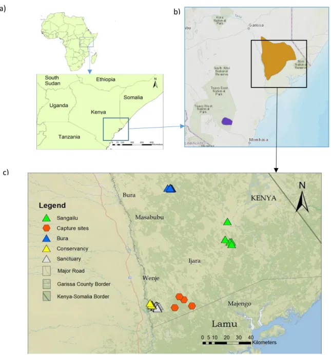
The Republic of Kenya is located in East Africa and is bordered to the north by Ethiopia and South Sudan, to the south and south-west by Tanzania, to the west by Uganda and to the east by Somalia and the Indic Ocean (Fig. 6a). The study area is focused in the eastern area of the Garissa County, which is situated in north-eastern Kenya and is bordered by Somalia (Fig. 6b).
Faecal samples were collected, in December 2017 and February 2018, from herds within the predator-free fenced sanctuary (1°52'24. 94"S 40°11'13. 55"E) and from wild herds outside the sanctuary at the Ishaqbini Community Conservancy (1°54'19. 56"S, 40°12'49. 89"E), and in Bura East (1º02’64’’S 40º30’83’’E) and Sangailu (1º40’20’’S 40º71’61’’E) administrative divisions (Figure 6b). A museum sample was retrieved from an individual hunted in the Bura area in 1937. Blood samples were obtained from individuals captured in 2012 near the Ishaqbini Community Conservancy (up to 30 km away from the sanctuary) and then translocated into the sanctuary (Figure 3b). Sampling was carried out by Dr. Abdullahi Ali (Founder of the Hirola Conservation Programme) and Matthew Mutinda (Field veterinary officer of Kenya Wildlife Service), together with local rangers. Eighteen hirola blood samples were retrieved from the group of 48 animals translocated into the sanctuary in August 2012, which were immobilized with a combination of 3 mg Etorphine hydrochloride (M99; a narcotic) and 30 mg Azaperone (Stresnil; a tranquilizer) with 6 mg Diprenorphine hydrochloride as a reversal. Faecal samples (n = 84) were collected from wild herds [Sangailu (n = 12) and Bura (n = 19) localities], from the sanctuary (n = 37) and from the conservancy (outside the sanctuary; n = 16). Hereafter, these groups are named as populations. Geographic coordinates were registered for most of the faecal samples (Missing: n = 5) and for the capture sites of the 2012 translocation. Blood samples were preserved in filter paper and faecal samples were preserved in plastic vials containing absolute ethanol. Samples were then sent to Research Centre in Biodiversity and Genetic Resources (CIBIO – InBIO Associate Laboratory).
2.2. DNA extraction and amplification
Small pieces of filter paper containing blood samples were cut and DNA was extracted using the EasySpin® Extraction Kit in columns for blood samples (QIAGEN, Germany), following manufacturer’s instructions. The success of DNA extraction was assessed through gel electrophoresis using a solution of agar at 0.8% and included GelRed Nucleic Acid Stain. DNA extraction from non-invasive (faeces) and museum samples was
Fig. 5- Study area and sampling: (a) The location (marked with a square) of the sampling area in Kenya, in East Africa, and neighbouring countries; (b) Map showing the current distribution of hirola (source: IUCN, 2017): the Tsavo population (dark blue) and the natural range (yellow), where the sampling occurred; (c) Map showing the location on which sampling of hirola scats took place (Sanctuary, Conservancy, Bura, Sangailu) and of the capture sites used for the 2012 translocation (into the sanctuary).
a) b)
performed in a laboratory facilities with sterile conditions and positive air pressure to reduce possible contaminations. The E.Z.N.A.® Tissue DNA Kit (Omega Bio-tek) was employed for faecal samples, following manufacturer’s instructions. An ancient DNA extraction protocol was used for the museum sample (Dabney et al., 2013) . Polymerase Chain Reaction (PCR) amplifications of nuclear and mitochondrial markers were conducted in a T100TM BIO-RAD 96 Well Thermal Cycler and included a negative control in each reaction to assess possible contaminations. In the case of faecal samples a positive control (a sample from Hippotragus niger variani) was also included. The success of PCR amplifications was assessed through gel electrophoresis using a solution of agar at 2% and GelRed Nucleic Acid Stain.
2.3. Amplification of mitochondrial DNA control region
Amplification of the mitochondrial DNA control region was divided in two overlapping fragments (named CR1 and CR2) to facilitate amplification of DNA from non-invasive samples (Table 1). Hirola specific primers were designed based on the complete mitochondrial genome of hirola available in GenBank (accession number: NC_023542).
Table 1- Description of primers and PCR conditions used to amplify the CR1 and CR2 fragments of the mitochondrial DNA control region.
Primer Primer sequence (5'-3') PCR conditions
CR1 F:aggaagaagctcatagccccac R:gcgagaagaggagtccctgcca 95ºC 15' 95ºC 30" (45 cycles) 48ºC 30" CR2 F:cgagcttaatcaccatgccgcgtg R:gtgccttgctttggttttaagc 72ºC 30" 60ºC 10' 10ºC FOREVER
Each 8 µl PCR contained approximately 3 µl of DNA, 5 µl Master Mix ( QIAGEN), 3,2 µl H20 and 0,4 µl of each primer (Forward and Reverse; diluted 1:10). PCR conditions were as follows: an initial denaturation step of 15 minutes at 95ºC; 45 cycles of denaturation at 95ºC for 30 seconds, annealing at 51ºC for 30 seconds and extension at 72ºC for 30 seconds; a final extension at 60ºC for 10 minutes. Following the PCR amplifications, an enzymatic clean-up using a mix of Exonuclease I and Thermosensitive Alkaline Phosphatase (both from Thermo Scientific) was performed in order to remove excess
primers and dNTPs. Conditions were as follows: 15 minutes at 37ºC and 15 minutes at 85ºC, following the manufacturer’s instructions. Samples were sequenced bi-directionally using the BigDye® Terminator v3.1 Cycle Sequencing Kit (Applied Biosystems), following the manufacturer’s protocol, and run on a 3130xl Applied Biosystems® automated sequencer. Chromatographs were checked manually, assembled, aligned and edited using Sequencher® (Gene Codes).
2.4.
Amplification of microsatellite markers from invasive
samples
As no primers were available specifically for hirola, a set of 72 cross-specific microsatellite markers developed for the giant sable (Hippotragus niger variani) (n = 58; Vaz Pinto et al., 2015), domestic sheep (Ovis aries; n = 10; International Society for Animal Genetics - ISAG ) and cattle (Bos Taurus; n = 4; ISAG) were tested for the 18 hirola blood samples. From the 72 markers tested, 44 were successfully amplified, although only 21 loci revealed to be polymorphic (see details in Table S1, Supplementary Material).
To overcome the poor quality of the amplifications, markers were amplified in a two-step PCR using a pre-amplification protocol and a M13 tailed primer (Piggott et al., 2004). Different mixes were used for pre and post PCRs. This was done for all multiplex PCRs with the exception of the cattle multiplex (see details in Table S2, Supplementary Material). For the pre-PCR, both the forward and reverse primers were used. For the post-PCR, only the reverse primer was used together with the M13-tail attached to the 5′ end. PCR amplifications were performed using approximately 3 µl DNA, 5 µl Master Mix (QIAGEN), 3,0 µl H20 and 1 µl of primer mixes (Table S1). Genotyping of PCR products was conducted on a 3130xl Applied Biosystems® automated sequencer using Gene ScanTM 500 LIZTM size standard (Thermo Fisher Scientific, United States of America). GeneMapper® v. 5.0 (Applied Biosystems™) was used to create bins, for each allele of each locus. Allele scoring was done through a semi-automated procedure, i.e. the automated allele calling done by the software was posteriorly checked through visual analysis in order to minimise scoring-related errors.
Departures from Hardy-Weinberg Equilibrium (HWE) were estimated for the 21 polymorphic markers using Genepop on the web v. 4.2 (Raymond & Rousset, 1995). Linkage disequilibrium (LD) between all pairs of loci was also computed in this software, with a dememorization number of 10,000, using 1,000 batches and 1,000 iterations per
batch. Significant departures from HWE or significant LD values were corrected applying a Bonferroni correction for tests with multiple comparisons (Dunn, 1958, 1961). Polymorphism information content (PIC) was calculated in CERVUS v3.0 (Kalinowski et al., 2007). Genetic diversity statistics per locus were calculated in GenAlEx v. 6.503 (Peakall & Smouse, 2012). These data were used for the selection of the most informative set of markers.
2.5. Amplification of microsatellite markers from non-invasive
samples and museum sample
Based on the PIC and after testing for HWE and LD, 14 out of the 21 polymorphic microsatellites were selected for genotyping non-invasive samples: HPN93, HpN12, HpN2, HpN9, Hpn16, HPN10, HSC, ILST87, Inra06, Inra5, BM1824, HPN13, HPN21 and TGLA53 (see more details in Table 2). PCRs reactions were conducted as described previously for the invasive samples, with Pre-PCR and Post-PCR procedures. However, as it is difficult to obtain reliable genotypes from non-invasive samples, a multiple-tubes approach (Taberlet et al., 1996) was used: DNA obtained from each faecal sample was amplified four times and a consensus genotype for each sample per locus was defined after comparing the different replicates. This was performed in GIMLET v1.3.3 (Valière, 2002), together with quantification of allele dropouts and false alleles. Departures from Hardy-Weinberg Equilibrium (HWE) were estimated using Genepop on the web v. 4.2 (Raymond & Rousset, 1995). Linkage disequilibrium (LD) between all pairs of loci was also computed in this software, with a dememorization number of 10,000, using 1,000 batches and 1,000 iterations per batch. Significant departures from HWE or significant LD values were corrected applying Bonferroni correction for tests with multiple comparisons (Dunn, 1958, 1961).