http://dx.doi.org/10.1590/S1982-21702013000400002
APPLICATION OF MEDIAN-EQUATION APPROACH FOR OUTLIER
DETECTION IN GEODETIC NETWORKS
Aplicação da equação mediana aproximada para a detecção de “outliers” nas redes geodésicas.
SERIF HEKIMOGLU BAHATTIN ERDOGAN
Department of Geomatic Engineering Yildiz Technical University, Istanbul, Turkey E-mail: [email protected] ; [email protected]
ABSTRACT
In geodetic measurements some outliers may occur sometimes in data sets, depending on different reasons. There are two main approaches to detect outliers as Tests for outliers (Baarda’s and Pope’s Tests) and robust methods (Danish method, Huber method etc.). These methods use the Least Squares Estimation (LSE). The outliers affect the LSE results, especially it smears the effects of the outliers on the good observations and sometimes wrong results may be obtained. To avoid these effects, a method that does not use LSE should be preferred. The median is a high breakdown point estimator and if it is applied for the outlier detection, reliable results can be obtained. In this study, a robust method which uses median with σ or
σ as a treshould value on median residuals that are obtained from median equations is proposed. If the a priori variance of the observations is known, the reliability of the new approch is greater than the one in the case where the a priori variance is unknown.
Keywords: Median; Median Absolute Deviation; Outlier; Median Equations; Decision Matrix; Leveling Network.
RESUMO
os resultados por contaminarem observações que são boas pelo efeito de espalhamewnto imposto pela LSE e às vezes resultados errados podem ser obtidos. Para evitar estes efeitos, um método que não usa LSE deve ser escolhido. A mediana é um estimados de pontos de grande valia e se é aplicado a um detector de erros grosseiros, resultados confiáveis podem ser obtidos. Nesta pesquisa, um método robusto que usa a mediana com σ ou σ é um valor que limita os resíduos medianos que podem ser obtidos a partir de equações medianas propostas. Se uma variância a priori das observações é conhecida, a confiabilidade do novo método é maior do que aquele, uja variância a prior é desconhecida.
Palavras-chave: Mediana; Derivação da Mediana Absoluta; Outlier; Equação Mediana; Matriz de decisão; Rede de Nivelamento.
1. INTRODUCTION
The least squares estimation (LSE) is very sensitive against deviations of the model assumptions (HAMPEL et al. 1986). The LSE spreads the effect of the outliers on the residuals of the good observations which do not have any outlier (HEKIMOGLU et al. 2011a). There are two main reasons for the wrong results of outlier detection methods as spreading effect of the LSE and weakness of configuration of the given geodetic network (HEKIMOGLU et al. 2011b). It is showed that an outlier in the observations of a geodetic network can not be identified reliably by using any method due to the configuration weakness in the network. The outlier affects badly the residual from LSE of another observation that lies close to this bad observation, due to the deficiency of the configuration of the network.
Generally, statistical procedures for detecting outliers work well in practice only in case of one single outlier, but can fail in case of multiple outliers (BAARDA 1968, POPE 1976, HEKIMOGLU and KOCH 1999 and 2000, XU 2005). In addition, Baselga (2007) showed that only one outlier in a geodetic network may be detected by using Test for outliers (Pope’s test) when the a priori variance of the observations is not known. In case of more than one gross error, the test becomes inefficient. Moreover, even the sample includes single outlier; the test may fail when observations are correlated. Tests for outliers are based on the assumption of a (possible) single outlier, and frequently with unjustified hope that they are supposed to be successful if multiple outliers appear. It is impossible to detect multiple outliers without additional hypotheses. Also, the single outlier hypothsis is also proven as being sufficient except to the case where the degree of freedom is one. These results of Baselga (2007 and 2011) verify the ones of the mentioned above properties.
location parameter (μ). However, the median is not as efficient as the mean, i.e. the standard deviation of the median is greater than the one of the mean at Gaussian distribution (MARONNA et al. 2006, p.20). Youcai (1995) applied the median and MAD (Median Absolute Deviation) to the triangulation network by identifying outliers under some criterions such as |ri|>2σmed or 3σmed where σmed =1.4826 MAD
and ri are the differences between the coordinates and the median of them. The
coordinates of the new points are calculated by taking all the possible combinations of observations (angles), and then the median applied to these coordinates’ values. Duchnowski (2010) applied R-Estimator to idendify unstable reference marks where the median and MAD play a main role.
Hekimoglu et al. (2011b) proved that the reasons for the failures in the outlier detection depend on not only due to the ability of the outlier detection method, but also mostly due to the weakness in the configuration of the networks. To detect the probable configuration weakness the median equations were used. In this paper, a new robust approach based on the median and MAD on the observations of the geodetic networks is introduced. To apply the median estimator for outlier detection the median equations are used. The main idea is to do outlier detection in geodetic networks that is based on observations without using LSE.
2. MEDIAN EQUATION APPROACH FOR LEVELING NETWORK
The geodetic networks are established to realize two main topics: estimating the coordinates of the new points optimally based on the coordinates of datum points, and controlling the reliability of the network whether the observations include outliers or not.
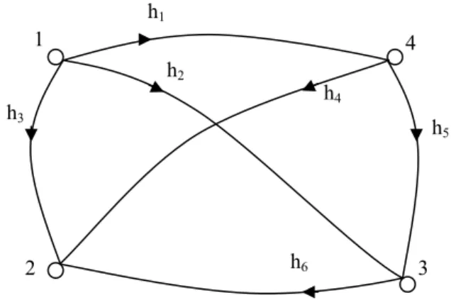
The height differences are measured for the leveling network. A minumum configuration that resists against one outlier is given in Fig. 1 (HEKIMOGLU et al. 2011b).
Figure 1 - A leveling network that has a minumum configuration that resists against one outlier.
1 4
2 3 h6
h1
h2
h3
h4
The following median equations can be written where each observation must appear once in these equations (HEKIMOGLU et al. 2011b):
(1a)
To clear this, an extra equation can be written such as:
h3 and h5 apper two times in these four equations. If h3 or h5 has an outlier, the
median can not separate them from the good observations. Therefore, the last equation can not be considered as a median equation. The similar median equations for the other observations can be written as follows:
,
(1b)
The median of these equations can be estimated such as:
, , , i=1,2,..,6 (2)
The median can separate only one outlier in these three median equations. For example, let h1 include an outlier. Med1 can separate it from two other median
equations. It can not affect Med1 and also Med2, Med3,…, Med6. Consequently, the
median can separate only one outlier in the observations of this leveling network. For example, if h1 and h5 were contaminated, the median can not separate these two
outliers.
Now, the question is arised how can this outlier be detected when the median is used as an estimator. If the variance σ2
of the population is known before, then the outlier may be detected by using the 3σ-rule (KUTTERER et al. 2003, LOON 2008).
Let h2 contaminated by outlier Δ. , , , and are damaged.
same sign (i.e. both + or both -) or Δ+ε < 3σ when both of them have the opposite sign (i.e. + and – or – and +). Therefore, more flagging values than the one may exceed the threshold value of 3σ. How can we decide which one of them is the true outlier? If the median equations of , , , and are considered, it is seen that they all include the common value of h2. Hence, the true bad observation
must be the value of h2. Thus, if observations have only one outlier and more
candidates of outlier are detected, true outlier can be found.
Let’slook at the leveling network given in Fig.1. We can obtain rij instead of
observations by using the Eq.(3):
, , , … ,6 , , , (3)
where rij are defined here as “median residuals”. They are considered here as
measuruments.
When h2 is contaminated by an outlier , , , and are
contaminated. As a result, 5 median equations of 18 are ruined by h2. The median of
rij is not affected by these five contaminated values. The main question is that how
we can detect the outlier in h2. According to the median equations we can form a
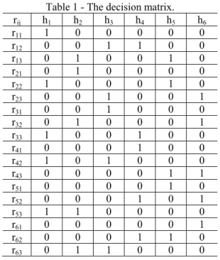
matrix which is called here “decision matrix” given Table 1. In the decision matrix, “0” means that there is no relation between observations and “1” means that these equations form one median equation (For example, in the second line of the matrix, r12 is formed by h3 and h4). When h2 is contaminated five median residuals (r13, r21,
r32, r53 and r63) are contaminated, too. According to the contaminated median
equations, for r13 h2 and h5; for r21 h2; for r32 h2 and h6; for r53 h2 and h1; for r63 h2 and
h3 can be flagged as outliers. The flagged means that this observation is set
candidate for contaminated observation. If the total flagged numbers is estimated, the number of h2 is five times, and other observations are only once, so that the
outlier can be detected considering decision matrix and total flagged number (k). If the total flagged number is bigger than one (k>1) this observation includes an outlier.
If the a priori variance σ2 is not known, σmed is proposed instead of MAD
because is more efficient than MAD (HAMPEL et al. 1986, ROUSSEEUW and LEROY 1987, MARONNA et al. 2006):
Table 1 - The decision matrix. rij h1 h2 h3 h4 h5 h6
r11 1 0 0 0 0 0
r12 0 0 1 1 0 0
r13 0 1 0 0 1 0
r21 0 1 0 0 0 0
r22 1 0 0 0 1 0
r23 0 0 1 0 0 1
r31 0 0 1 0 0 0
r32 0 1 0 0 0 1
r33 1 0 0 1 0 0
r41 0 0 0 1 0 0
r42 1 0 1 0 0 0
r43 0 0 0 0 1 1
r51 0 0 0 0 1 0
r52 0 0 0 1 0 1
r53 1 1 0 0 0 0
r61 0 0 0 0 0 1
r62 0 0 0 1 1 0
r63 0 1 1 0 0 0
3. SIMULATION OF THE LEVELING NETWORK
To apply the new median approch, the network given in Fig.1 is considered. The heights of four points are H1=100.000 m, H2=105.276 m, H3=104.388 m and
H4=103.055 m respectively. They are not affected from random errors. The height
differences (hoi, i=1,2,..,6) are computed. To obtain the measurements of the height
differences we assume that the random measurement errors have the same variance σ2 (i.e. σ=1 mm). Thus, the measurements of the height differences h
i are computed
as
, , , … ,6 (6)
where ei ~ N(μ=0, σ2=1), it is assumed that the measurement errors are Gaussian
with the expected value which is equal to zero and the variance which is equal to 1. Here ei are 0.90, -0.52, -0.50, -0.97, 0.00, 1.39 mm
To generate one contaminated height value , the random error ei is replaced
by the outlier dhi as follows:
, , , … ,6 (7)
I. The observations do not include any outlier.
II. The observation (h1) is contaminated with +5 mm magnitude.
III. The observation (h1) is contaminated with +10 mm magnitude.
IV. The observation (h1) is contaminated with +1000 mm magnitude
which is called as a wild observation.
For the first case: The median equations for each height difference hi are
constituted and their medians are taken according to the equations of (1a), (1b) and (2). Then, the differences (rij) according to (3) are computed. σmed of them is found
as 1.0 mm. The method did not detect any outlier which is greater than for the case when the a priori variance is known, and also for the case when the a priori variance is unknown.
For the second case: The median residuals (rij) according to Eq. (3) are given
as [-4.5, 0.0, 0.9, 0.0, -5.5, 1.4, 1.4, 0.0, -3.2, 0.0, 4.5, -2.3, -2.4, 0.0, 3.2, -1.4, 0.9, 0.0] mm. If we look at rij-values, we can see that the outlier is not spreaded on the
adjacent observations as in LSE. The σmed of them is 2.0 mm. The threshold value
for rij is 3 mm for . We see that there are five values (r11, r22, r33, r42 and r53)
greater than . These median equations are contaminated by h1. The height
difference h1 is the joint value among these five contaminated values. In the
decision matrix h1 is flagged five times and h2, h3, h4, h5 and h6 are flagged only
once, since the flagged number of the h1 is greater than one, h1 is the outlier. If the a
priori variance is unknown, is used as a threshold value. Since none of the median residuals exceed the the method can not detect the outlier.
For the third case: The differences (rij) according to Eq. (3) are given as [-9.5,
0.0, 1.0, 0.0, -10.5, 1.4, 1.4, 0.0, -8.2, 0.0, 9.5, -2.4, -2.4, 0.0, 8.2, -1.4, 1.0, 0.0] mm. The σmed of them is 2.0 mm again. If the a priori variance σ2 of the height
differences is known, is used as threshold value that is the same as in second case. We see that there are five values (r11, r22, r33, r42 andr53) that are greater than
. h1 is the joint observation. In the decision matrix h1 is flagged five times and h2,
h3, h4, h5 and h6 are flagged only once, since the flagged number of the h1 is greater
than one h1 is the outlier. If the variance σ2 of the height differences is unknown,
is used as a threshold values that are the same as in second case. We see that there are five values (r11, r22, r33, r42 andr53) that are greater than . If we look at
these median equations, there is one joint value i.e. h1 among them. Therefore, h1
must be contaminated.
For the fourth case: The differences (rij) according to (3) are given as [-999.5,
0.0, 1.0, 0.0, -1000.5, 1.4, 1.4, 0.0, -998.2, 0.0, 999.5, -2.4, -2.4, 0.0, 998.2, -1.3, 1.0, 0.0] mm. If we look at rij values, we can see that the outlier is not spreaded on
the adjacent observations as in LSE. The σmed of them is 2.0 mm again. There are
five values (r11, r22, r33, r42 andr53) that are greater than . If we see these median
equations, there is one joint value h1. Thus, we can detect this outlier in h1. If the a
priori variance σ2
values (r11, r22, r33, r42 andr53) that are greater than . If we see these median
equations, there is one joint value h1. Therefore, h1 must be contaminated.
We see that the σmed value for the cases II, III and IV does not change as the
magnitude of outlier changes. This is the proof for the property of robustness.
4. SIMULATION RESULTS
We know that the success of the robust methods and Tests for outliers are changed from one sample to the other one where the random errors are different (HEKIMOGLU and KOCH 1999, HEKIMOGLU and KOCH 2000). Therefore, the success of a method used cannot be evaluated by the result from one sample which may be chosen subjectively.
For simulation the network given in Fig.1 was considered. The random errors, 6 mesurements and outlier are generated as done in above section. They come from a Gausian distribution such as N(μ, σ2
=1mm2). A hundered random error vectors e and also a hundered good sample are generated. In addition, each sample is contaminated only by one outlier 100 times. Thus, we have obtained 10 000 contaminated samples.
rij are analysed by using median and threshold value as or . The
results are given in Table 2. To measure the capacity of a method, the mean success rate (MSR) (HEKIMOGLU and KOCH 1999, HEKIMOGLU and KOCH 2000, HEKIMOGLU and ERENOGLU 2007, ERENOGLU and HEKIMOGLU 2010) is used.
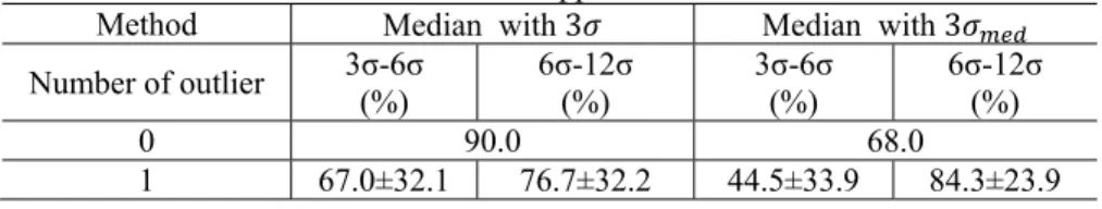
Table 2 - MSRs and standard deviations of the new median equation approach.
Method Median with Median with
Number of outlier 3σ-6σ (%)
6σ-12σ (%)
3σ-6σ (%)
6σ-12σ (%)
0 90.0 68.0
1 67.0±32.1 76.7±32.2 44.5±33.9 84.3±23.9
Considering the algorithm of forming the median equations, i.e. the decision matrix which gives us how the height differences in the median equations are connected, we can detect outlier when the repeat number k of the flagged outliers is greater than 1. If the median and median equations are used for outlier detection the reliability of the method in condition that a priori variance is known is 67% where the magnitude of an outlier lies between and 6 . If the a priori variance is unknown the reliability of the method decreases to 44.5%. The method may detect the good observations as outliers for some cases.
5. CONCLUSION
In this study, it is investigated that whether median (with 3σ or 3σmed) may be
consid which The fla be see outlier results a prior used. I the a p
REFE BAAR P C BASE J BASE D DUCH C V EREN te V HAMP s N HEKIM b G HEKIM b HEKIM h 1 HEKIM “ S HEKIM " 4 KUTT D
dering the algo gives us how agged numbe en how many r can be detec s of the levelin ri variance σ2
If σmed is used
priori variance
ERENCES RDA W. (19 Publication o Commission, D ELGA S. (2007
J. Surv. Eng. 1 ELGA S. (20
Detection in L HNOWSKI R Controlling R Vol.136(2):47-NOGLU R. C. ests for outlie Vol. 45(4): 426 PEL F., RON
tatistics: the
New York MOGLU S., K be measured?”
Gründing (Eds MOGLU S., K be measured?, MOGLU S., heterogeousne 37-148 MOGLU S., “Increasing th Survey Review MOGLU S., Detecting Con 43 (323): 713-TERER H., HE Detection in V
orithm of for w the height d r of the obser y times a mea cted when the ng network, th of the observ d the MSRs d e σ2 is known.
968), “A test on Geodesy,
Delft. 7), "Critical li
33(2): 52–55 11), "Non Ex east Squares A R. (2010), “M
Reference M -52
, HEKIMOG ers for geode 6-439 NCHETTI E.,
approach bas
KOCH K. R. ”, in Third T
s), 1-4 June,Is KOCH K. R.
Allg. Vermes
ERENOGLU ss on outlier
ERDOGAN B he reliability
w ,Vol. 46(3):2 ERENOGLU nfiguration W 730.
EINKELMAN VLBI Data An
rming the med differences in rvation is obta asurement is e flagged num he median me vations is know decreases by c
ting procedur
New Series
imitation in us
xistence of R Adjustment", Median-Based Mark Stabili
LU S., (2010 etic adjustmen
ROUSSEEU
sed on influen
(1999), “How
Turkish Germ
stanbul, Turke (2000) “How
. Nachr., 107( U R. C. (2007
detection for
B., ERENOG of the tests f 291-308 U R. C., SAN Weaknesses in
NN R., AND nalysis” Proc
dian equatios, the median e ained from the flagged in th mber is greate ethod can be u
wn. If it is no comparing the
re for use i
s 2, no.5.,
se of test fo
Rigorous Tes
J. Surv. Eng., Estimates an ity”, J. of
0), “Efficiency nt models, Ac
UW P., STAH
nce functions"
w can reliabilit
man Joint Geo
ey, 179-196. w can reliabilit
(7): 247-254, 7), “Effect of
geodetic netw
GLU R. C., H for outliers fo
NLI D. U., E Geodetic Net
TESMER V.
ceedings of th
, i.e. the decis equations are e decision ma his decision m er than 1. Acc used especiall ot known, σmed
e ones of the
in geodetic N Netherlands
or gross error
sts for Multip , 137(3): 109-nd Their App
f Surv. En
y of robust m
cta.Geod. Geo
HEL W. (1986 ", John Wiley
ty of the robu
odetic Days,
ty of the test
f heterosceda works, J.Geod
HOSBAS R. G for geodetic n
ERDOGAN B tworks", Surv
(2003), “Rob
he 16th Workin
sion matrix connected. atrix. It can matrix. The cording the y when the
d should be
case where Networks”, Geodetic detection". ple Outlier 112 plication in ngn.-ASCE, methods and
oph. Hung.
6), "Robust
y and Sons,
ust methods
Altan and
for outliers
asticity and
desy, 81(2):
G. (2011a), netwowks”,
B., (2011b),
vey Review,
bust Outlier
on European VLBI for Geodesy and Astrometry, W. Schwegmann and V. Thorandt, eds., Bundesamt für Kartographie und Geodäsie, Leipzig/Frankfurt, 247-255.
LOON J. P. (2008), “Functional and stochastic modelling of satellite gravity data,
Publications on Geodesy 67, Netherlands Geodetic Commission, Delft. MARONNA R., MARTIN D., YOHAI V. (2006), "Robust Statistics", Wiley, New
York.
POPE A. J. (1976), "The statistics of residuals and the outlier detection of outliers"
NOAA Technical Report, NOS 65, NGS 1, Rockville, MD.
ROUSSEEUW P. J., LEROY A. M. (1987), "Robust regression and outlier detection", John Wiley and Sons, Inc., New York.
XU P. L. (2005), “Sign-constrained Robust Least Squares, Subjective Breakdown Point and the Effect of Weights of Observations on Robustness”, Journal of Geodesy 79:146-159
YOUCAI H. (1995), "On the design of estimators with high breakdown points for outlier identification in triangulation Networks", Bull. Geod. 69:292 – 299