www.atmos-chem-phys.net/7/443/2007/ © Author(s) 2007. This work is licensed under a Creative Commons License.
Atmospheric
Chemistry
and Physics
Water-side turbulence enhancement of ozone deposition to the ocean
C. W. Fairall1, D. Helmig2, L. Ganzeveld3, and J. Hare4,* 1NOAA Earth Science Research Laboratory, Boulder, CO, USA 2INSTAAR, University of Colorado, Boulder, CO, USA 3Max-Planck Institute for Chemistry, Mainz, Germany 4CIRES, University of Colorado, Boulder, CO, USA
*now at: SOLAS International Project Office, University of East Anglia, Norwich, UK
Received: 3 March 2006 – Published in Atmos. Chem. Phys. Discuss.: 26 June 2006 Revised: 4 December 2006 – Accepted: 15 January 2007 – Published: 25 January 2007
Abstract. A parameterization for the deposition velocity of an ocean-reactive atmospheric gas (such as ozone) is de-veloped. The parameterization is based on integration of the turbulent-molecular transport equation (with a chemical source term) in the ocean. It extends previous work that only considered reactions within the oceanic molecular sublayer. The sensitivity of the ocean-side transport to reaction rate and wind forcing is examined. A more complicated case with a much more reactive thin surfactant layer is also considered. The full atmosphere-ocean deposition velocity is obtained by matching boundary conditions at the interface. For an as-sumed ocean reaction rate of 103s−1, the enhancement for ozone deposition by oceanic turbulence is found to be up to a factor of three for meteorological data obtained in a recent cruise off the East Coast of the U.S.
1 Introduction
The transport, formation and depletion of ozone have re-ceived significant research attention because of the recog-nized importance of ozone for the chemical and radiative properties of the atmosphere. Ozone is the most impor-tant precursor of the OH radical in the troposphere. Both ozone and OH are fundamental for the oxidizing capacity of the atmosphere and their concentrations determine the re-moval rates of many atmospheric contaminants. Increased anthropogenic emissions of nitrogen oxides and hydrocar-bons, both being precursors of photochemical ozone produc-tion in the atmosphere, have led to significant increases in global, surface-level ozone concentrations. It has been esti-mated that tropospheric ozone has at least doubled since pre-industrial times (Lamarque et al., 2005). Observations from background monitoring sites indicate that ozone continues Correspondence to:C. W. Fairall
(chris.fairall@noaa.gov)
to rise (Oltmans et al., 1998; Vingarzan, 2004; Helmig et al., 2007). Previous and anticipated future increases in back-ground tropospheric ozone are a concern for several reasons. Ozone is a toxin to humans and animal life on Earth. Further-more, tropospheric ozone has a significant (∼13%) contribu-tion to anthropogenic greenhouse gas forcing (IPCC, 2001), which possibly might further increase in the future due to continued increases in ozone and concomitant reductions in the growth rates of other important greenhouse gas emis-sions. These unique roles of ozone in atmospheric chem-istry have motivated a plethora of research on improving our understanding of formation, transport and loss processes of atmospheric ozone.
Observed deposition velocities are reported in the litera-ture with values ranging fromVd∼0.01 to 0.12 cm s−1 for ocean water and 0.01–0.1 cm s−1for fresh water (Ganzeveld
et al., 20071). This literature gives little details on the chemical, biological and physical water properties during the observations. Currently, values on the order of Vd=0.013 to 0.05 cm s−1 are used in atmospheric chemistry models (Ganzeveld and Lelieveld, 1995; Shon and Kim, 2002). Be-cause the observations do not yield a consensus on wind speed dependency, the same ozone surface resistance is typ-ically applied to all of the world’s oceans and wind condi-tions.
In general, the deposition of ozone involves both turbu-lent and molecular diffusive plus chemical processes in air and water. If atmospheric chemical reactions are negligi-ble (see Lenschow, 1982; Geernaert et al., 1998; Sorensen et al., 2005, for counter examples), then the atmospheric part of the problem can be treated with standard similarity the-ory (Fairall et al., 2000). In the near-surface region, ver-tical turbulent diffusion in both fluids exhibits near-linear height/depth dependence associated with restriction of ed-dies by the presence of the boundary. Furthermore, the vis-cosity of a turbulent fluid causes dissipation of the turbulence that is more intense the smaller the turbulent eddy. This leads to a turbulent microscaleδu≈10ν/u∗(νis the fluid kinematic viscosity andu∗the friction velocity) such that the spectrum of turbulent fluctuations for eddies smaller thanδu is expo-nentially attenuated. Because of this suppression of turbu-lent eddies near the boundary, ozone entering the water from the air is initially transported away from the interface solely by molecular diffusion. This interfacial region dominated by molecular transport is called the molecular sublayer. The time scale associated with random molecular transport over a distanceδ istD=δ2/Dx whereDx is the molecular diffu-sivity of the gas,X, in the fluid. If the time scale of some chemical reaction forXwithin the fluid can be characterized by 1/a, then in the absence of turbulent effects, we expect the reaction to be substantially completed within a distance
δ=[Dx/a]1/2. Becauseδuis about 10−3m, this simple scale analysis suggests that for ozone turbulent transport effects need not be considered whenaexceeds about 100 s−1.
Garland et al. (1980) used a horizontally homogeneous conservation equation to link the oceanic chemical reactivity of ozone to the oceanic deposition resistance by solving the case where δ≪δu (i.e., turbulent diffusion was neglected). Schwartz (1992) discussed the more general problem of the balance of solubility and aqueous reaction kinetics from the point of view of chemical enhancement of solubility for re-versible reactions for a variety of gases. Chemical enhance-ment refers to an apparent increase of the solubility of the
1Ganzeveld, L., Helmig, D., Fairall, C. W., and Pozzer, A.:
Biogeochemistry and water-side turbulence dependence of global atmospheric-ocean ozone exchange, Global Biogeochem. Cycles, in preparation, 2007.
gas by reactions in the water. The context for that discus-sion was thestagnant filmmodel, which is equivalent to ne-glecting turbulent transport in the aqueous phase. In the irre-versible limit, Schwartz’s results for ozone reduce to the Gar-land result. More recently, Chang et al. (2004) expanded the scope to combine molecular diffusive - chemical and turbu-lent diffusive - chemical processes as parallel resistances. In this approach, the oceanside stagnant film resistance of Gar-land et al. (1980),Rg, acts independently and in parallel with a Schmidt-number dependent oceanic resistance,Rw, taken from Wanninkhof (1992) but which includes a chemical en-hancement factor:Rc=(1/Rw+1/Rg)−1. Chang et al. (2004) also discuss various oceanic chemicals that are expected to be the reacting agent (iodide being the strongest candidate).
Recent research on ocean-atmosphere gas and energy ex-change has resulted in improved models that describe the de-pendencies of deposition on atmospheric and oceanic pro-cesses from a more fundamental perspective (Fairall et al., 2000; Hare et al., 2004). In this paper, we will apply this for-malism to a trace atmospheric gas that reacts chemically in the ocean. We extend the approach of Garland et al. (1980) to the case where not all of the gas reacts within the molecular sublayer. Whereas Chang et al. (2004) postulate that the de-position velocity is a combination of independent parallel re-sistances, we derive the deposition velocity analytically from the fundamental conservation equations (albeit in simplified form). Their approach includes a characteristic reaction con-stant,a, plus the chemical enhancement factor,β; in our ap-proach, the “enhancement” effect is a natural consequence of the solutions to the budget equation.
2 Conservation equation
Using the notation from the 2000 Fairall et al. paper, the budget equation for the mass concentration of some chemi-cal,Xw, in water is
∂Xw/∂t+U· ∇Xw= −
∂hw′x′
w−Dxw∂Xw/∂z
i
∂z −aXw (1)
wherezis the vertical coordinate (distance from the inter-face, i.e.,depthfor the ocean),U the mean horizontal flow,
w′x′
wthe turbulent flux (positive downward),Dxwthe molec-ular diffusivity ofXin water, and the last term is the loss rate ofXwdue to reactions with some chemicalYw. We represent the turbulent flux in terms of an eddy diffusion coefficient,
w′x′
w=−K∂X∂zw, whereK(z)is the turbulent eddy diffusiv-ity,
∂Xw/∂t+U· ∇Xw= −
∂[−(Dxw+K(z))∂Xw/∂z]
∂z −aXw (2)
a flux variable,Fxw, which, in dynamic equilibrium, is con-stant:
−[Dxw+K(z)]∂Xw/∂z+a z
Z
0
Xw(z)dz=Fxw. (3)
This flux variable is the sum of transport (mixing) fluxes by molecular diffusion,FxD, and turbulent diffusion,FxT, plus an apparent flux associated with the decreasing concentration of ozone as it enters and penetrates the ocean and is destroyed by reaction withY.
To apply Eqs. (2) and (3) to the case of an inert or weakly reacting gas, we leta=0. This simplifies the analysis because we can directly write an equation for the concentration dif-ference:
∂Xw
∂z =
Fxw
Dxw+K(z)
(4a)
Xws−Xw(zr)=Fxw zr
Z
0
dz Dxw+K(z)
=Fxw
δu
Z
0
dz Dxw+K(z)
+ zr
Z
δu
dz Dxw+K(z)
(4b)
From Eq. (4b) the resistance law analogy becomes apparent where the total resistanceRxw (which is the inverse of the transfer velocity,Vxw)is the sum of the molecular diffusion sublayer resistance,Rxwm, and the turbulent layer,Rxwt,
Xws−Xw=FxwRxw=Fxw(Rxwm+Rxwt)=Fxw/Vxw (5) HereRxwmis the integral over the velocity diffusion sublayer andRxwt the integral from the top of the turbulent layer to the reference depth.
We can write a similar equation for the transport ofX in the atmosphere (Fairall et al., 2000). Conventionally, the at-mospheric equation is defined with the vertical ordinate as height above the interface and transport fluxes are defined positiveupwardso that the flux in the atmosphere associated with deposition to the surface is given by
Fxa = −VdxXa= −Fxws (6)
whereXais the mass concentration at some reference height in the atmosphere andFxws is the flux into the water at the air-water interface. In equilibrium, the oceanic total flux (re-member, this flux is the sum of local transport and accu-mulated loss ofXvia chemical reaction) is independent of depth, soFxws=Fxw. As in Eq. (5) the atmospheric flux can be characterized by an atmospheric-side transfer veloc-ity and the difference in the concentration at the interface and the reference height
Fxa =Vxa(Xas−Xa)=
(Xas−Xa)
(Rxam+Rxat)
(7)
In the absence of atmospheric chemical reactions, the
Ra=Rxam andRb=Rxat terms would follow from integrat-ing Eq. (4b) with the normal similarity relations (Fairall et al., 2000). A similar relationship applies for the ocean side
Fxa = −Fxws = −Vxw(Xws−Xw) (8) Using the solubility relationshipXws=Xas∗αx, whereαx is the dimensionless solubility ofX, we can eliminate the surface concentrations and derive a general flux relationship in terms of the atmospheric and oceanic gas concentrations
Fxa =
(Xw/αx−Xa)
(Ra+Rb)+(αxVxw)−1
(9) Note that Eq. (9) can be applied even if there is a chemi-cal reaction in the ocean, but the interpretation of the atmo-spheric resistance as a sum of molecular and turbulent dif-fusion sublayer components only follows directly from the budget equation for a non-reactive atmosphere. For the de-position problem where ozone is destroyed by chemical re-action in the ocean,Xw=0, it follows that
Rc−1=αxVxw=αxFxws/Xws (10a)
Vdx =(Ra+Rb+Rc)−1 (10b)
3 Oceanic transfer velocity from the budget equation
In this section we will solve the basic conservation equation for ozone entering the ocean from the atmosphere. To sim-plify the notation, we will drop thewsubscripts in this sec-tion because it deals only with oceanic processes.
3.1 Negligible turbulence solution
In the limit that the reaction is so strong that the profile of
Xw becomes negligible within the oceanic molecular sub-layer (besides ozone, other obvious examples include HNO3
and SO2; the paradox that ozone is both strongly reacting in
the ocean and is ocean-transfer limited is caused by its weak solubility), we can neglect theKterm and write
Dx
∂2X
∂z2 −aX=0 (11)
Assuming that the concentration ofY is much larger thanX
so that it remains effectively constant, the solution is (Gar-land et al., 1980)
X=Xsexp
−
r a
Dx
z
(12) whereXs is the concentration ofXat the water surface. The diffusive flux at any depth in the fluid is
FxD(z)= −Dx
∂X
∂z = −Dx ∂ ∂z
Xsexp
−
r a
Dx
z
=Xs
p
aDxexp
−
r a
Dx
z
0 0.5 1 1.5 2 2.5 3 0
1 2 3 4 5
x K n
(x) and I
n
(x)
I 0
I 1 K
1
K 0
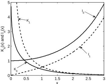
Fig. 1.Graphical representations of the Modified Bessel Functions of order 0 and 1 for the dimensionless variable,x(order 0: solid line and order 1: dashed line).
The diffusive flux is a function of depth but at the interface (z=0)
FxD(0)=Fxs=Xs
p
aDx (14)
From Eq. (10) it immediately follows that
Vxw=Fxs/Xs =
p
aDx (15)
3.2 Non-negligible turbulence solution
To consider the turbulent transport case, we first specify a simple form for the turbulent eddy diffusivity that is obtained from surface-layer similarity scaling (Fairall et al., 2000)
K(z)=κu∗z. Here we have neglected buoyancy (stability ef-fects),κ=0.4 is the von Karman constant, andu∗is the fric-tion velocity in theoceansurface layer. If we do not neglect turbulent transport, then Eq. (2) becomes
∂ ∂z
(Dx/κu∗+z)
∂X ∂z
− a
κu∗X=0 (16)
If we transform to y2=(Dx/κu∗+z), then the solutions are modified Bessel functions of zero order (Geernaert et al., 1998)
X=AI0(ξ )+BK0(ξ )
ξ2= 4a
κu∗
z+ Dx
κu∗
(17) Details on modified Bessel functions of ordern,InandKn, can be found in Abramowitz and Stegun (1964); examples forn=0 and 1 are shown in Fig. 1. To determineAandB, we invoke the boundary conditions. Ifais uniformly distributed throughout the ocean, the boundary conditions are defined at the interface (z=0) and infinitely deep in the ocean (z→∞)
Deep Ocean: X(z)→0; z→ ∞ (18a)
Surface: − [Dx+K(z)]
∂X
∂z =Fxs; z→0 (18b)
BecauseI0becomes large aszincreases, condition Eq. (18a)
impliesA=0. If we assume thatX=B*K0(ξ ). In terms of K0, the total mixing component of the flux is
FxM =FxD+FxT = −(Dx+κu∗z)
∂X ∂z
= −B(Dx+κu∗z)
∂K0(ξ )
∂z (19)
Writing this in terms of the variableξ, we use the property ofK0so that−ξ∂K∂ξ0=K1to describe the mixing component
as a function of depth
FxM
B = − (κu∗)2
4a ξ
2∂K0(ξ ) ∂ξ
∂ξ ∂z
= −(κu∗)
2
4a ξ
2∂K0(ξ ) ∂ξ
2a κu∗ξ
−1= κu∗
2 ξ K1(ξ ) (20) We then determine the constantB by evaluating Eq. (20) at the surface (condition 18b)
B= 2Fxs/κu∗
ξ0K1(ξ0)
(21) where
ξ0=
2
κu∗
p
aDx (22)
Determination ofBallows us to explicitly write the equation for the profile ofX in the water. We substitute Eq. (21) in Eq. (17a) withA=0:
X(z)= 2Fxs/κu∗
ξ0K1(ξ0)
K0(ξ ) (23)
And the profile of the mixing component of the flux
FxM(z)=Fxs
ξ K1(ξ )
ξ0K1(ξ0)
(24) Notice that Eq. (24) describes howFxM(z)declines as the gas is absorbed; the decline of the mixing flux is balanced by destruction ofX by chemical reaction. A bit of algebra shows that Eq. (3) can be written
Total Flux=
ξ K1(ξ )+
ξ
Z
ξ0
ξ K0(ξ )dξ
Fxs
ξ0K1(ξ0)
(25)
The first term is the transport (turbulent plus molecular diffu-sion) and the second is the loss by chemical reaction. Far into the water, the transfer term becomes 0 and the flux entering the fluid has all been consumed:
Fxs =a
∞
Z
0
X(z)dz= κu∗ 2 B
∞
Z
ξ0
Through the properties of Bessel functions,
ξ K0(ξ )=−∂(ξ K∂ξ1(ξ )), Eq. (26) provides an alternate method
to relateBto the surface flux.
The water-side transfer velocity is obtained simply from using Eq. (23) in Eq. (15)
Vxw=
κu∗
2
ξ0K1(ξ0) K0(ξ0)
=paDx
K1(ξ0) K0(ξ0)
(27) The limiting values of Bessel functions are well known, so we can examine Eq. (27) in the limit whereais large; in this case,ξ0is large and the ratioK1/K0=1. Thus, we recover the
Garland et al. (1980) solution given in Eq. (15). The profile ofX(z)in the diffusion sublayer is given by Eq. (4) and the concentration ofXapproaches 0 forz>Dx/κu∗.
For small values ofa, we find that
Vxw→ −
κu∗
2 ln
2
κu∗
p
aDx
(28) In this regime the profile of X is linear in the diffusion sublayer and then logarithmic in z and approaches 0 for
z≈κu∗/4a=δT. The transition between strongly and weakly reacting regimes occurs forξ0≈1
acrit= (κu∗)2
4Dx
(29) Typical open ocean values (κu∗w≈0.0037 ms−1 and
Dozone≈3.0 10−9m2s−1) in Eq. (29) give the transition
around acrit≈1000 s−1. Ganzeveld et al. (2007)1 find the
value of a for ozone considering the Iodide-DMS-alkene chemistry never exceeds 1000 s−1. Introducing highly-parameterized DOM-O3 chemistry based on the chlorofyll concentrations, it is exceeded for some confined regions close to coasts. Ifa significantly exceeds acrit, then ozone
is consumed within the oceanic diffusion sublayer. The dimensionless parameter ξ0 defined in Eq. (22) is, in fact,
the ratio of the chemo-molecular diffusive scaleδD defined in the Introduction and the chemo-turbulent diffusive scale
δT defined above.
3.3 Two-layer reactivity (surfactant) solution
In this section we examine a more complicated vertical dis-tribution of reactivity designed to mimic assumed properties of a highly reactive surfactant. A surfactant may be a hy-drophilic material that tends to have much enriched concen-tration at the surface or a soluble compound that influences some surface property of seawater (e.g., viscosity or surface tension). We do not say what this surfactant is but specify its properties as having reactivityabeginning at the interface and down to a depthδrelative to some background reactivity
aothat is present everywhere. Here we consider a two-layer solution
Layer I: 0< z < δ
where reactivity =a+ao X(z)=AII0(ξ )+BIK0(ξ )
(30a)
Layer II: z > δ
where reactivity =aoX(z)=BI IK0(ξ ) (30b)
In layer I the solutions are described by Eq. (17a) butAis not 0; in layer IIA=0.
In order to find the values of the three coefficients, we must match three boundary conditions: (1) the flux at the surface, (2) the continuity of concentration at the I-II boundary, and (3) the surface flux must equal the total absorption ofXby reaction in the medium. For the general form ofX(z), the transport flux is
FxM(z)=
κu∗
2 [−Aξ I1(ξ )+Bξ K1(ξ )] (31) The three boundary conditions can be written as follows: −AIξ0I1(ξ0)+BIξ0K1(ξ0)=
2Fxs
κu∗ AII0(ξδ)+BIK0(ξδ)−BI IK0(ξδ)=0
AI(a+a0)
δ
Z
0
I0(ξ )dz+BI(a+a0)
δ
Z
0
I0(ξ )dz
+BI Ia0 ∞
Z
δ
K0(ξ )dξ =Fxs (32)
Alternatively, a flux continuity condition at the I–II inter-face can be substituted for any one of these equations. The three relationships from Eq. (32) can be written as the prod-uct of a 3X3 matrix times a coefficient vector = flux vector (H∗A=F):
h11 h12 h13 h21 h22 h23 h31 h32 h33
∗
AI
BI
BI I
=
2Fxs
κu∗
0
Fxs
(33)
where thehij coefficients come from the terms in Eq. (32). The coefficients are found by inverting the H matrix,
A=H−1∗F. Once the coefficients are obtained, the
water-side transfer velocity is given by
Vxw=
p
(a+a0)Dx
[−AII1(ξ0)+BIK1(ξ0)]
[AII0(ξ0)+BIK0(ξ0)]
(34)
4 Discussion
10−2 10−1 100 101 102 103 104 10−3
10−2 10−1 100
a (s−1)
α
Vw
(cm s
−1
)
u* = 0.5 m/s
u* = 0.035 m/s
No Turbulence Theory
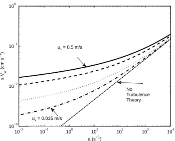
Fig. 2. Water-side transfer velocity (multiplied by solubility) for ozone from Eq. (27) as a function of reactivity, a. The indi-vidual curves are for different values of friction velocity: solid:
u∗a=0.5 ms−1; dashed: u∗a=0.3 ms−1; dotted: u∗a=0.1 ms−1; dashdot:u∗a=0.035 ms−1. The dots with the thin line are the no-turbulence solution.
wind speed of 10 ms−1. If we assume the atmospheric stress
drives an equal turbulent stress in the ocean, then the oceanic friction velocity follows from the ratio of the densities
u∗w=
rρ
a
ρw
u∗a≈u∗a/30≈0.0012U10 (35)
The curves in Fig. 2 are bounded on the bottom by the no-turbulence (stagnant film) theory of Garland et al. (1980). The family of curves spans wind speeds from about 1.0 to 15 ms−1. For strong winds the oceanic transfer velocity is
much more weakly dependent ona. Regarding thetotal at-mospheric deposition velocity, interpretation of the implica-tions of Fig. 2 requires specification of the atmospheric trans-fer. We use the NOAA-COARE gas transfer model (Fairall et al., 2000; Hare et al., 2004)
Rxa =Ra+Rb=
Cd−1/2+13.3Sca1/2−5+
log(Sca) 2κ
/u∗a
(36) where Cd is the momentum drag coefficient at the refer-ence height and Sca the Schmidt number for ozone in air (about 1). In Eq. (36) the Cd term representsRa and the remaining terms representRb. For an atmospheric reference height of 10 mCd−1/2≈28; at a wind speed of 10 ms−1the
at-mospheric resistanceRa+Rb≈100 sm−1, implying a trans-fer velocity of about 1.0 cms−1. Typical observed ozone total deposition values are on the order of 0.05 cms−1 (to-talR=2000 sm−1), so we know thatRc dominates the total transfer resistance. From Fig. 2 we can see that 0.05 cms−1 corresponds toa≈103s−1.
100 101
10−1 100
Vt
(cm s
−1
)
U10 (m s−1)
Fig. 3. Total deposition velocity as a function of wind speed for ozone using Eq. (10) witha=1000 s−1. The solid line is the at-mospheric component,Rxa, from Eq. (36). The dashed line isVd combining Eq. (36) with Eq. (27) forVxw; the line with circle sym-bols isVdcombining Eq. (36) with stagnant film result (Eq. 15); the line with x’s isVdfrom Chang et al. (2004).
BecauseVdfor ozone is usually dominated by the oceanic component, it is clear from Fig. 2 that ocean turbulence prob-ably plays a significant role in the variability of ozone deposi-tion. This conclusion follows from the observed wind-speed dependence ofVd because the stagnant film result (Eq. 16) is independent of wind speed. An alternative explanation is thata systematically increases with wind speed, which con-tradicts the conventional wisdom that surfactants are more prevalent in light winds. Figure 3 shows wind speed de-pendencies obtained using Eq. (27) in Eq. (9) when specify-inga=103s−1. Note the atmospheric transfer velocity (solid line) is about 10 times larger than the effective oceanic veloc-ity. Thus, for this value ofa, the ocean is the dominant bottle-neck to transfer;awould have to be two orders of magnitude larger for the oceanic and atmospheric resistances to be com-parable. The wind-speed dependence of the no-turbulence theory for Vd is very weak because it enters only through the atmospheric component (Eq. 15), which does not depend onu∗. The model of Chang et al. (2004), which empirically incorporates ocean turbulence in a less rigorous way, gives results that are fairly similar to Eq. (27).
The surfactant case has been examined by specifying a background valuea0=10−4s−1to the result of a thin layer
of thickness 10−5m of surfactant as suggested by Schwartz
com-10−6 10−4 10−2 100 102 104 10−3
10−2 10−1
α
Vw
(cm s
−1
)
Surfactant a (s−1) Background a = value on x−axis
Background a = 1E−4 s−1
2−layer solution
Fig. 4. Water-side transfer velocity (multiplied by solubility) for ozone as a function of reactivity, a, for u∗a=0.035 ms−1. The flat solid line denotes the velocity with a fixed background at
a=a0=10−4; the dotted line denotes the velocity computed with
Eq. (27) withataking the values on the x-axis. The dashed line with plus symbols denotes the velocity computed using Eq. (34) with a surfactant layer 10−5m thick with reactivity on the x-axis which is added to the background value.
parable fora on the order of 1000 s−1. This suggests that observed values of ozone deposition velocities could be the result of a thin layer of surfactant (i.e., deep layers are not required) as suggested by Schwartz (1992).
The one-layer ozone deposition velocity parameterization has been coded in Matlab and Fortran90 in a form that is easily paired with the NOAA-COARE bulk flux algorithm (Fairall et al., 2003). In addition to the normal near-surface variables needed for bulk fluxes (i.e., in the COARE algo-rithm), inputs are required forαx , a, andScw . For illus-tration we have computed transfer velocities from a recent field program on the NOAA ShipRonald H. Brownthat was conducted off the coast of New Hampshire in July and Au-gust 2004. Further details on the measurements and the field program are available at http://www.etl.noaa.gov/programs/ 2004/neaqs/flux/. The bulk meteorological variables mea-sured from the ship are input to the NOAA-COARE flux al-gorithm and then the meteorological fluxes are used to com-pute the ozone deposition velocity. Deposition velocities are computed for a 16-day period after specifying αx=0.3,
a=103s−1, andScw=500 (Fig. 5). The no-turbulence model shows little variation except for occasional periods of lighter winds and strong atmospheric stability (warm air over cool water) where hydrostatic stability effects suppress bothu∗
and the atmospheric transfer.
190 195 200 205
0 0.005 0.01 0.015 0.02 0.025 0.03 0.035 0.04 0.045 0.05
Vd
(cm s
−1
)
Julian Day (2004)
Fig. 5. Time series of ozone deposition velocity computed from bulk meteorological measurements from a recent cruise of the NOAA ShipRonald H. Brownoff New England in July and Au-gust 2004. The thick line is Vd computed with using Eq. (15) with Eq. (36), which neglects turbulent transport in the ocean; the thin dashed line is Eq. (27) with Eq. (36), which includes turbulent transport in the ocean. Ozone variables are specified asαx =0.3,
a=103s−1, andScw=500.
5 Conclusion
Starting from the fundamental conservation equation, we have derived relationships for the deposition velocity of ozone to the ocean that accounts for the oceanic chemical destruction. This work has several implications for interpre-tation and planning of field observations. Typical deposition values quoted in the literature imply that the atmospheric re-sistance is small compared to the oceanic rere-sistance. Further-more, the atmospheric resistance is well-characterized after decades of study of temperature, moisture, and trace gas in-vestigations. Thus, oceanic mechanisms dominate the uncer-tainty in the parameterization of ozone deposition to the sea. This uncertainty involves not only the normal complexity of oceanic mechanisms such as breaking waves and oceanic bubbles (see Fairall et al., 2000) but the additional uncer-tainty associated with variability in the near-surface chemical reactions. The value of reactivity (a=103s−1)that is consis-tent with observations of ozone deposition velocity suggest a thin ozone penetration depth in the ocean that could be pro-vided by a surfactant microlayer. However, our results show that even in that case oceanic turbulent mixing will still play a role in deposition (e.g., Fig. 3).
global characterizations of near-surface chemistry relevant to ozone oceanic transfer (see Ganzeveld et al., 20071).
The algorithms and data used in this example are available at the following ftp site:
ftp://ftp.etl.noaa.gov/user/cfairall/bulkalg/gasflux/ozone/.
List of Symbols
a Chemical reactivity in the ocean (s−1)
acrit Value of a where molecular and turbulent diffusive
mechanisms are comparable
t Time (s)
u∗ Friction velocity;u∗=p−w′u′(ms−1) u∗a Friction velocity for air
u∗w Friction velocity for water
u′ Horizontal velocity turbulent fluctuation w′ Vertical velocity turbulent fluctuation
x′ Turbulent fluctuation of concentration X
w′x′ Turbulent covariance (vertical flux) of gas X w′u′ Turbulent stress or covariance of vertical and
hor-izontal velocity fluctuations
z Vertical coordinate, depth in water and height in air (m)
zr Reference depth (or height in air) far from the in-terface where bulk concentration is measured
A Coefficient theI0Bessel function term
AI Coefficient theI0Bessel function term in layer I
(surfactant layer)
AI I Coefficient theI0Bessel function term in layer II
(bulk layer)
B Coefficient theK0Bessel function term
BI Coefficient theK0Bessel function term in layer I
(surfactant layer)
BI I Coefficient theK0Bessel function term in layer II
(bulk layer)
Cd Momentum transfer (drag) coefficient
Cxy Rate coefficient for reaction of X and Y, a=CxyYw
Dx Molecular diffusivity for gas X (m2s−1)
Dxa Molecular diffusivity for gas X in air
Dxw Molecular diffusivity for gas X in water
Fx Mass flux variable for gas X (kgm−2s−1)
Fxs Mass flux variable for gas X at the air-water inter-face
Fxa Mass flux variable for gas X in air
Fxw Mass flux variable for gas X in water
FxD Mass flux variable for gas X associated with the molecular diffusion term
FxT Mass flux variable for gas X associated with the turbulent diffusion term
FxM Mass flux variable for gas X by mixing, =FxD +
FxT
In,Kn Modified Bessel functions of ordern
K(z) Turbulent eddy diffusion coefficient (m2s−1) R Transfer resistance (sm−1)
Ra Transfer resistance for the atmospheric turbulent sublayer
Rb Transfer resistance for the atmospheric molecular sublayer
Rc Transfer resistance for the ocean
Rg Transfer resistance for the ocean from ozone reac-tivity from Garland et al. (1980)
Rw Transfer resistance for the ocean for mixing from Wanninkhof 1992
Rxt Transfer resistance for the atmospheric turbulent sublayer computed via Eq. (4b)Rxt a=Ra
Rxm Transfer resistance for the atmospheric molecular sublayer computed via Eq. (4b)Rxma=Rb
Scx Schmidt number=ν/Dxfor gas X
Sca Schmidt number=νa/Dxafor gas X in air
Scw Schmidt number=νw/Dxwfor gas X in water
U Horizontal fluid velocity, wind speed or current speed (ms−1)
U10 Wind speed at a reference height of 10 m Vd Deposition velocity
Vdx Deposition velocity for gas X
Vxa Transfer velocity for gasXin air, =1/Rxa
Vxw Transfer velocity for gasXin water, =1/Rxw
Xa Concentration ofXin air (kgm−3)
Xw Concentration ofXin water (kgm−3)
Xas Concentration ofXin air at the air-water interface (kgm−3)
Xws Concentration ofXin water at the air-water inter-face (kgm−3)
Yw Concentration of the chemical Y that reacts with
Xin the water (kgm−3)
αx Dimensionless solubility for gasX in the ocean, =Xws/Xas
β Chemical enhancement factor where solubility is replaced byβαx
δ Transport sublayer thickness (m)
δu Turbulent microscale or velocity sublayer thick-ness
δD Chemo-diffusive sublayer thickness for molecular diffusion
δT Chemo-diffusive sublayer thickness for turbulent diffusion
κ von Karman constant (=0.4)
Acknowledgements. This work is supported by the NOAA Office of Global Programs (Carbon Cycle program element), the NOAA Health of the Atmosphere program, and NSF award CHE-BE #0410048. Any opinions, findings, and conclusions expressed in this material are those of the authors and do not necessarily reflect the views of the funding agencies.
Edited by: M. Heimann
References
Abramowitz, M. and Stegun, I. A.: Handbook of Mathematical functions. Applied Mathematics Series, 55. US Gov. Printing Of-fice, Washington, DC, 1964.
Chang, W., Heikes, B. G., and Lee, M.: Ozone deposition to the sea surface: chemical enhancement and wind speed dependence, Atmos. Environ., 38, 1053–1059, 2004.
Fairall, C. W., Hare, J. E., Edson, J. B., and McGillis, W.: Parame-terization and micrometeorological measurements of air-sea gas transfer, Bound.-Layer Meteorol., 96, 63–105, 2000.
Fairall, C. W., Bradley, E. F., Hare, J. E., Grachev, A. A., and Ed-son, J. B.: Bulk parameterization of air-sea fluxes: Updates and verification for the COARE algorithm, J. Clim., 16, 571–591, 2003.
Ganzeveld, L. and Lelieveld, J.: Dry deposition parameterization in a chemistry general circulation model and its influence on the distribution of reactive trace gases, J. Geophys. Res., 100, 20 999–21 012, 1995.
Garland, J. A., Etzerman, A. W., and Penkett, S. A.: The mecha-nism for dry deposition of ozone to seawater surfaces, J. Geo-phys. Res., 85, 7488–7492, 1980.
Geernaert, L. L. S., Geernaert, G. L., Granby, K., and Asman, W. A. H.: Fluxes of soluble gases in the marine atmospheric surface layer, Tellus B, 50, 111–127, 1998.
Hare J. E., Fairall, C. W., McGillis, W. R., Edson, J. B., Ward, B., and Wanninkhof, R.: Evaluation of the National Oceanic and Atmospheric Administration/Coupled-Ocean Atmospheric Re-sponse Experiment (NOAA/COARE) air-sea gas transfer param-eterization using GasEx data, J. Geophys. Res., 109, C08S11, doi:10.1029/2003JC001831, 2004.
Helmig, D., Oltmans, S. J., Carlson, D., Lamarque, J.-F., Jones, A., Labuschagne, C., Anlauf, K., and Hayden, K.: A review of surface ozone in the polar regions, Atmos. Environ., in press, 2007.
IPCC Climate Change 2001: A report by the Working Group I of the Intergovernmental Panel on Climate Change, http://www. ipcc.ch/, 2001.
Lamarque, J.-F., Hess, P., Emmons, L., Buja, L., Washing-ton, W., and Grainer, C.: Tropospheric ozone evolution between 1890 and 1990, J. Geophys. Res., 110, D08304, doi:10.1029/2004JD005537, 2005.
Lenschow, D. H.: Reactive trace species in the boundary layer from a micrometeorological perspective, J. Meteorol. Soc. Japan, 60, 472–480, 1982.
Liss, P.: Processes of gas exchange across an air-water interface, Deep-Sea Res., 20, 221–228, 1973.
Oltmans, S. J., Lefohn, A. S., Scheel, H. E., Harris, J. M., Levy II, H., Galbally, I. E., Brunke, E. G., Meyer, C. P., Lathrop, J. A., Johnson, B. J., Shadwick, D. S., Cuevas, E., Schmidlin, F. J., Tarasick, D. W., Claude, H., Kerr, J. B., Uchino, O., and Mohnen, V.: Trends of ozone in the tropopsphere, Geophys. Res. Lett., 25, 139–142, 1998.
Schwartz, S.: Factors governing dry deposition of gases to surface water, in: Precipitation Scavenging and Atmosphere–Surface Exchange, vol. 2. edited by: Schwartz, S. and Slinn, S., Hemi-sphere Publishing Corp., Washington, USA, pp. 789–801, 1992. Shon, Z.-H. and Kim, N.: A modeling study of halogen chemistry’s role in marine boundary layer ozone, Atmos. Environ., 36, 4289– 4298, 2002.
Sorensen, L. L., Pryor, S. C., De Leeuw, G., and Schulz, M.: Flux divergence of nitric acid in the marine atmospheric surface layer, J. Geophys. Res., 110, D15306, doi:10.1029/2004JD005403, 2005.
Vingarzan, R.: A review of surface ozone background levels and trends, Atmos. Environ., 38, 3431–3442, 2004.
Wanninkhof, R.: Relationship between wind speed and gas ex-change over the ocean, J. Geophys. Res., 97, 7373–7382, 1992. Wesely, M. L. and Hicks, B. B.: A review of the current status of