M
ODELLING AND ANALYSIS OF
FOREST FIRE IN
P
ORTUGAL
- P
ART
I
Giovani L. Silva
CEAUL & DMIST - Universidade Técnica de Lisboa gsilva@math.ist.utl.pt
Maria Inês Dias & Manuela Oliveira CIMA & DM - Universidade de Évora
misd@uevora.pt & mmo@uevora.pt
Susete Marques & José Borges ISA - Universidade Técnica de Lisboa smarques@isa.utl.pt & joseborges@isa.utl.pt
In the last decade forest fires became a serious problem in Portu-gal due to different issues such as climatic characteristics and nature of Portuguese forest. In order to analyse forest fire data, we use gen-eralized linear models for modeling the proportion of burned forest area. Our goal is to find out fire risk factors that influence that pro-portion of burned area and what may make a forest type susceptible or resistant to fire. Then, we analyse forest fire data in Portugal during 1990-1994 through frequentist and Bayesian approaches.
Keywords: Fire management, Burned area proportion, Forest fire data, Generalized linear model.
1
I
NTRODUCTION
In Portugal, forest fires and the related burned area have been increasing in the last years, as opposed to other southern European countries. Fire is indeed an important issue in Mediterranean region affecting the ecological and economic aspects of forest areas and causing loss of human life. Many factors have contributed to the increasing number of forest fires, e.g., cli-mate change. [7] identified changes in the number of fires, burned area and fire size distribution depending on topographical variables and vegetation type in a Spanish region.
The motivating application is the analysis of forest fire data in the en-tire Portuguese mainland between 1990 and 1994. There were 5,706 fires
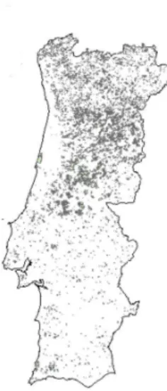
in Portugal during that period burning about 4.97% of the country area. Figure 1 displays the distribution of these fires identifying high and critical fire risk zones that are specially located in the northern and central interior of Portugal. [6] pointed out many causes and consequences of forest fires in Portugal. Namely, Portuguese forest is mainly based on a monoculture of pine and eucalyptus, which are highly combustible species due to their essential oils.
Figure 1: Distribution of forest fires in Portugal (1990-1994).
For analyzing forest fire data, generalized linear models (GLM) are usu-ally adopted[1]. The goal of this work is to model the proportion of burned area analyzing high dimensioned forest fire data in Portugal. The rest of the article is organized as follows. Section 2 succinctly describes a few GLM for the burned area proportion. In Section 3 we present the corresponding re-sults of data analysis and some discussion. A second spatio-temporal data analysis is done in Section 4 in order to identify temporal trends and pro-duce smoothed maps including regional effects, including model selection for the burned area in Portugal from a Bayesian point-of-view.
2
S
TATISTICAL MODEL
Portuguese mainland covers about 90,000 km2 in southern Europe. Most of the country is included in the Mediterranean region and the altitudes range from sea level to about 2,000 m. For the analysis of the forest fires in Portugal, the forest was initially divided into classes of altitude (m), slope (%), slope orientation or aspect, population (hab/km2), proximity to roads,
number of days with precipitation greater than 1 mm, number of days with maximum temperature higher than 25oC, and fuel (Table 1).
Proximity Population Slope Altitude Aspect Precipitation Temperature ≥ 1000 < 25 0−10 < 200 plane 0−6 0−3 < 1000 25−100 10−20 200−400 north 7−13 4−48 > 100 20−30 400−700 east 14−18 49−71 > 30 > 700 south 19−22 72−92 west 23−26 93−112 ≥ 27 ≥ 113
Fuel: no fuel, annual crop, eucalyptus, hardwoods, hardwoods and softwoods mixed with eucalyptus (HSME), agro-forestry, permanent crop, shrubs, resinous or softwoods (RS), softwoods mixed with eucalyptus (SME).
Table 1: Description of the classes used in the forest fire study.
Secondly, we record the observed proportion of burned forest area, de-noted by ri that is the burned area out of total area for the ith combination of levels for the covariates in study, i= 1, . . . , k. There are several GLM to model the proportion of burned area from these eight underlying covari-ates. For instance, using the logit transformation of ri, one has
yi ≡ log(ri/(1 − ri)) = z0iβ + εi, (1)
where the random errorsεi, i=1, . . . , k, may be considered (independent) Gaussian random variables with mean zero and variance σ2, and β is the regression coefficient vector associated with the observed covariate vector
zi. Notice that the eight covariates in Table 1 give rise to thirty two dummy variables.
Other transformations may be adopted for ri, such as, arcsin(pri) and Box-Cox transformations. One can make inference on regression parameter
β in (1) based on classical [1] and Bayesian [3] methods for GLM. For the
latter, the prior distributions may be flat but proper Gaussian and inverse gamma priors for regression parameters and variance, respectively.
3
F
IRST RESULTS AND DISCUSSION
Let M1 denote model (1) with all covariates showed in Table 1, whereas
M2 and M3represent the corresponding models with arcsin(pri) and Box-Cox transformations, respectively. The Akaike Information Criterion (AIC) values for the models M1, M2 and M3 are respectively 50350, 58815 and
57613, pointing to the M1 model. We also fitted and compared other re-duced models for example the model M4, which is the model M1 without the covariates slope orientation, precipitation and maximum temperature.
In addition, we explore a Bayesian approach for model M1, assuming Gaussian prior with mean zero and variance 106for the regression parame-ters and inverse gamma with shape and scale parameparame-ters equal to 0.001 for the variance σ2. Based on Deviance Information Criterion (DIC), the best model is M1 (DIC=149011) in comparison with M4 (DIC=152481). Then, we decided to select model M1 because DIC is a generalization of AIC that handles hierarchical models of any degree of complexity[3].
For simplicity, Table 2 only displays the model parameter estimates for
M1 from a Bayesian perspective: posterior mean and 95% credible inter-vals (CI) for the regression parameters and variance σ2. Note that Markov chain Monte Carlo (MCMC) samples of size 10,000 were obtained for M1, taking every 10th iteration of the simulated sequence, after 5,000 itera-tions of burn-in[8]. A study of convergence of the samples was carried out using several diagnostic methods and none of them showed any worrying features.
According to model M1 (Table 2), there is only no significant effect of annual and permanent crop fuels and precipitation 14−18 on the propor-tion of burned forest area in Portugal during 1990-1994. The proporpropor-tion tends to increase with slope, altitude, road proximity and even precipita-tion, whereas populaprecipita-tion, aspect and temperature display a decreasing ef-fect in the posterior mean of yi. The areas with larger likelihood to have for-est fires are (in increasing order) softwoods mixed with eucalyptus (SME), eucalyptus, shrubs, resinous or softwoods (RS), hardwoods and softwoods mixed with eucalyptus (HSME), hardwoods, and agro-forestry.
This preliminary analysis of forest fire data in Portugal helps us to figure out the influence of the observed combinations of risk factors (k=25, 388) on the proportion of burned forest area. However, further research is being developed for capturing the spatio-temporal effect on the proportion [2] or using more proper distributions and link functions, e.g., Beta regression [5].
4
S
PATIO
-
TEMPORAL MODELLING
In order to identify temporal trends and produce smoothed maps including regional effects, we also recorded the proportion of burned area by districts or municipalities and year in mainland Portugal during 1990 and 2006 (sec-ond data analysis). There are 18 districts and 278 municipalities in Portu-gal.
Parameter Mean 95% CI Parameter Mean 95% CI intercept 10.120 9.524 10.72 Precipitation Road prox. 7−13 -0.225 -0.409 -0.031 < 1000 0.133 0.020 0.247 14−18 0.116 -0.075 0.302 Population 19−22 0.784 0.586 0.978 25−100 -0.311 -0.575 -0.263 23−26 0.590 0.379 0.796 ≥ 100 -0.423 -0.436 -0.179 ≥ 27 0.811 0.570 1.039 Slope Temperature 10−20 1.025 0.902 1.148 4−48 -9.837 -10.2 -9.456 20−30 2.746 2.571 2.925 49−71 -10.08 -10.45 -9.706 ≥ 30 8.362 7.947 8.769 72−92 -10.07 -10.45 -9.684 Altitude 93−112 -8.361 -8.89 -7.885 200−400 0.611 0.450 0.768 ≥ 113 -10.22 -10.89 -9.533 400−700 0.796 0.630 0.960 Fuel ≥ 700 1.796 1.613 1.969 annual crop -0.231 -0.502 0.036 Aspect eucalyptus 1.953 1.664 2.252 north -5.806 -6.198 -5.408 hardwoods 0.729 0.449 1.013 west -5.945 -6.332 -5.554 HSME 1.353 1.068 1.640 east -5.932 -6.319 -5.541 agro-forestry 0.302 0.011 0.584 south -5.999 -6.395 -5.603 permanent crop -0.107 -0.415 0.197 shrubs 1.860 1.610 2.126
σ2 20.7 20.35 21.05 RS 1.767 1.498 2.032
SME 2.232 1.923 2.537
Table 2: Estimates of the regression parameters and variance for model M1.
Let ri t denote the proportion of the burned area out of the regional size for region i at time t, i= 1, . . . , n, t = 1, . . . , T. Similarly, we may assume the transformed ri t ( yi t) is Gaussian distributed.
Generalized spatial mixed models account for correlation among regions by using random effects. A general spatiotemporal model for area i at time
t is
yi t≡ logit ri t = α0+ S0(t) + Si(t) + bi+ hi+ εi t, (2) where S0(t) is the overall trend in the odds, Si(t) is the regional specific trend, and bi (hi) is a spatially correlated (unstructured) random effect [10]. For current fire data, there are n = 18 districts and T = 17 years (1990-2006).
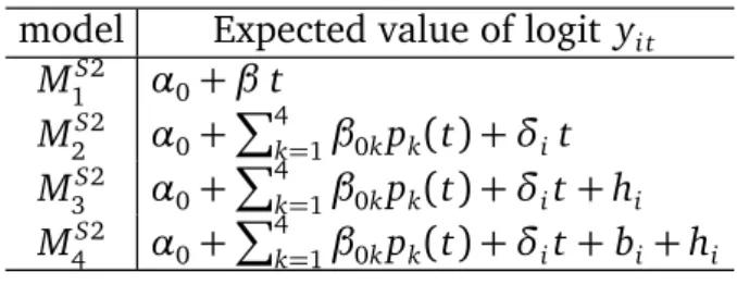
Table 3 displays different specifications of model (2), e.g., simple linear trend MS2
1 and nonlinear overall and linear regional trends M S2 4 .
Spline smoothing may reveal nonlinear temporal effects for both tem-poral and spatiotemtem-poral components. Cubic B-splines (no intercept and
model Expected value of logit yi t
M1S2 α0+ β t
M2S2 α0+ P4k=1β0kpk(t) + δi t M3S2 α0+ P4k=1β0kpk(t) + δit+ hi M4S2 α0+ Pk4=1β0kpk(t) + δit+ bi+ hi
Table 3: Several spatio-temporal models (2).
one inner knot) can be assumed for the arbitrary smoothing function S0(t), where pk(·) are the spline basis functions and β0k the corresponding coeffi-cients.
For the likelihood, we can assume different distributions for the propor-tion of burned area ri or ri t. For instance,
1. Gaussian distribution (µ, σ2) for log(r/(1 − r)). 2. Gamma distribution (c, d) for− log(r).
3. Beta distribution (a, b), with mean µ = a/(a + b) and variance µ(1 −
µ)/(1 + γ), where γ may interpreted as a precision parameter (for µ
fixed, largerγ implies smaller Var(r)).
Although the third option above does not seem difficult for implemen-tation, we found out some problems especially when we calculated some summary measures of model comparison. Thus, we decided to present here inference based on the first one. More research needs to be done for using that distribution in spatiotemporal modeling.
In Bayesian analysis, we usually assume independent normal distribu-tions with zero mean and variances w2
j for the regression coefficients, if there are. Considering cubic B-splines for S0(t), the corresponding spline basis coefficients β0k would be also assigned independent normal distribu-tions with zero mean and variances vk2, k=1, . . . , 4. For unstructured spatial heterogeneity hi, we assume an independent normal distribution, i.e.,
hi|σh2 ∼ Normal(0, σ 2
h). (3)
If Si(t) = δit in (2), one may also assume that δi ∼ N (0, σ2δ), i = 1, . . . , n, independently, and independent of bi and hi.
Further prior assumption: using an intrinsic conditional autoregressive (CAR) model [4] for spatially structured components bi in (2), the condi-tional distribution of bi is
bi|b−i,σ2b ∼ Normal(¯bi,σ 2
where ¯bi = Pj∈Ni bj/ni, Ni denotes the set of labels of the “neighbors” of
area i, ni is the number of areas which are adjacent to area i, b−i denotes b without bi, andσ2bis a variance component. In fact, the spatially correlated vector b = (b1, . . . , bn) has a multivariate normal distribution with zero-mean vector and covariance matrixσ2bQ−1, where Q has diagonal element
Qii= ni and the off-diagonal element Qi jis 1 if regions i and j are neighbors and 0 otherwise, i, j=1, . . . , n.
For the hyperparameters σ2b and σ2h (variance components), as well as the variance of linear regional trend effectσ2δ, one usually assigns an inverse gamma prior, i.e.,
• σ2
b ∼ I G(c1, d1) • σ2
h∼ I G(c2, d2) • σ2δ∼ I G(c3, d3).
The variance parameters are in fact assigned highly dispersed, but proper inverse gamma, whereas regression coefficients and B-spline coefficients have similarly normal priors. Assuming a priori independence amongst the model parameters, we can construct the joint posterior density related to spatio-temporal model (2).
The joint posterior distributions are usually awkward to work with, since the marginal posterior distributions of some parameters are not easy to ob-tain explicitly. These posteriors can be evaluated using Markov chain Monte Carlo (MCMC) methods. In particular Gibbs sampling works by iteratively drawing samples for each parameter from the corresponding full condi-tional distribution, which is the posterior distribution condicondi-tional upon cur-rent values of all other parameters. Fitting the curcur-rent model via MCMC methods, we can estimate quantities of interest, e.g., the “relative” spatial odds for area i defined by exp(bi + hi).
Model comparison: An important issue is to choose among postulated sub-models of the models (1) or (2), especially because certain Bayesian spatiotemporal model choice techniques are not applicable[?]. Some sum-mary measures of model comparison are easily evaluated with MCMC meth-ods, e.g., the posterior mean of Deviance D(θ ). Deviance information cri-terion defined by
DI C = 2 D(θi t) − D(θi t), (5)
where D(θi t) and θi t denote the posterior mean of the deviance and the model parameter θi t, respectively. It is a generalization of the Akaike in-formation criterion (AIC) for handling hierarchical Bayesian models of any degree of complexity.
In fact, we assumed Gaussian priors with mean zero and variance 106for
βj’s and inverse gammas with shape and scale parameters equal to 0.001 for the variance σ2. MCMC samples of size 10,000 were obtained for all models, taking every 10th iteration of the simulated sequence, after 5,000 iterations of burn-in. A study of convergence of the samples was carried out using several diagnostic methods and none of them showed any worrying features.
Table 4 lists some sub-models of spatiotemporal model (2) (increasing level of complexity). MS2
4 is identified consistently as the selected model. Note that the models were fitted via MCMC methods implemented in GeoBugs [11].
Models defined from l o g i t yi t D DIC
MS2
1 : α0+β t 1401.47 1404.4
M2S2: α0+S0(t)+δi t 1381.85 1390.8
M3S2: α0+S0(t)+δi t+hi 1272.30 1297.5
M4S2: α0+S0(t)+δi t+bi+hi 1271.85 1294.4 Table 4: Several fitted spatio-temporal models (2).
Parameter specification: β and β0k (spline coefficients) and σ2b, σ 2 h, andσ2
δ(variance hyperparameters) have highly dispersed priors, i.e., N(0, 105) and I G(0.5, 0.0005), respectively. The overall trend effect (exp(α0+S0(t))) indicates increasing “overall” odds of burned area after 2000 up to 2003 and some departures from logit-linearity, being slower than the overall lin-ear increase from 1993 to 2000 and faster between 2000 and 2005 (Figure 2). 1990 1995 2000 2005 0.000 0.005 0.010 0.015 0.020 year
overall trend effect
model M1 model M4
Figure 2: Overall trend effect S0(t).
In order to identify regions with significant district temporal trends, 95% HPD credible intervals were also obtained for exp(δi) based on model M3.
None was considered linearly significant. Maybe, we should also have as-sumed a nonlinear district temporal effect.
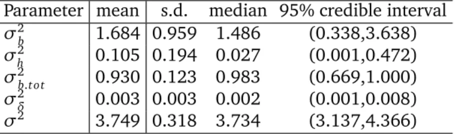
Table 5 provides estimates of the variance components for model MS2 4 . Note that σ2 b.t ot = σ 2 b/(σ 2 b+ σ 2
h) is interpreted as the relative importance of the variance component of the spatially correlated effects versus the to-tal spatial variance component. There is significant heterogeneity but the greatest influence arises from spatial correlation. Figure 3 displays esti-mates of the spatial effects exp(bi+ hi) (model MS2
4 ).
Parameter mean s.d. median 95% credible interval
σ2 b 1.684 0.959 1.486 (0.338,3.638) σ2 h 0.105 0.194 0.027 (0.001,0.472) σ2 b.t ot 0.930 0.123 0.983 (0.669,1.000) σ2 δ 0.003 0.003 0.002 (0.001,0.008) σ2 3.749 0.318 3.734 (3.137,4.366)
Table 5: Variance components for model M4S2.
Figure 3: Spatial random effects.
Some remarks and future works: i) We identified changes in the propor-tion of burned area depending on topographical variables and vegetapropor-tion type. ii) Spatiotemporal models produce smoothed estimates of the nonlin-ear overall or small-area specific temporal effects in mapping proportions over time and yield informative interpretations of the data. iii) For fire data analysis, we provided mechanisms for isolating small-area trends of
importance in this study. iv) It is missing a sensitivity analysis for prior as-sumptions, especially for the hyperparameters. v) We must consider a mass of probability for no fire ignition (ri = 0) as spatialtemporal modeling by municipalities (see Amaral-Turkman er al., 2011).
A
CKNOWLEDGEMENTS
This paper was partially supported by Pest-OE/MAT/UI0006/2011.
R
EFERENCES
[1] Amaral-Turkman M.A. and Silva, G.L. (2000). Modelos Lineares
Gener-alizados - da teoria à prática, Portuguese Statistical Society, Portugal. [2] Amaral-Turkman M.A., Turkman K.F., Le Page, Y. and Pereira, J.M.
(2011) Hierarchical space-time models for fire ignition and percent-age of land burned by wildfires, Environmental and Ecological
Statis-tics, 18, 601-617.
[3] Banerjee S., Carlin B. and Gelfand A.E. (2004) Hierarchical Modeling
and Analysis for Spatial Data, Chapman and Hall/CRC, Boca Raton, Florida.
[4] Besag, J., York, J., and Mollié, A. (1991). Bayesian image restoration with two applications in spatial statistics (with discussion), Ann. Inst.
Stat. Math., 43, 1-59.
[5] Ferrari S.P. and Cribari-Neto F. (2004) Beta regression for modelling rates and proportions, Journal of Applied Statistics, 31, 799-815. [6] Gomes J.F.P. (2006) Forest fires in Portugal: how they happen and
why they happen, International Journal of Environmental Studies, 63, 109-119.
[7] González J.R. and Pukkala T. (2007) Characterization of forest fires in Catalonia (northeast Spain), European Journal of Forest Research, 126, 421-429.
[8] Lunn, D.J., Thomas, A., Best, N. and Spiegelhalter, D. (2000). Win-BUGS – a Bayesian modelling framework: concepts, structure, and extensibility, Statistics and Computing, 10, 325-337 (http://www.mrc-bsu.cam.ac.uk/bugs/).
[9] Marques, S., Borges, J. G., Garcia-Gonzalo, J., Moreira, F., Carreiras, J.M.B., Oliveira, M.M., Cantarinha, A., Botequim, B. and Pereira, J.M.C. (2009). Characterization of wildfires in Portugal. European
Journal of Forest Research, 130, 775-784.
[10] Silva, G.L., Dean, C.B., Niyonsenga, T. and Vanasse, A. (2008). Hi-erarchical Bayesian spatiotemporal analysis of revascularization odds using smoothing splines, Statistics in Medicine, 27, 2381-2401. [11] Thomas, A., Best, N., Lunn, D., Arnold, R., and Spiegelhalter, D.