“Dedolomitization reactions¿? driven by anthropogenic activity on loessy sediments, SW Hungary

“DEDOLOMITIZATION REACTIONS” DRIVEN BY ANTHROPOGENIC ACTIVITY ON LOESSY SEDIMENTS, SW HUNGARY

RE-REVISED VERSION – AG-05-1708

by

Fernando A. L. Pacheco1,* and Teodora Szocs2

1

Geology Department and Centre for Chemistry, Trás-os-Montes and Alto Douro University, Ap. 1013, 5000 Vila Real, Portugal.

2

HydrogeochemicalDepartment, Geological Institute of Hungary, 1143-H, Budapest, Stefánia út 14, Hungary * Corresponding author

ABSTRACT

In the Szigetvár area, SW Hungary, shallow groundwaters draining upper Pleistocene loess and Holocene sediments are considerably contaminated by domestic effluents and leachates of farmland fertilizers. The loess contains calcite and dolomite, but gypsum was not recognized in these sediments. The anthropogenic inputs contain significant amounts of calcium and sulfate. The calcium from these anthropogenic inputs is promoting calcite growth, with concomitant consumption of carbonate alkalinity, undersaturation of the system with respect to dolomite, and dolomite dissolution; in brief, is driving “dedolomitization reactions”. Geochemical arguments supporting the occurrence of “dedolomitization reactions” in the area are provided by the results of mass balance and thermodynamic analyses. The mass balances predicted the weather

sequence dolomite > calcite > plagioclase > K-feldspar, at odds with widely accepted sequences of weatherability where calcite is the first mineral in the row. The exchange between calcite and dolomite can be a side effect of “dedolomitization reactions” because they cause precipitation of calcite. The thermodynamic prerequisites for “dedolomitization reactions” are satisfied by most local groundwaters (70%) since they are supersaturated (or in equilibrium) with respect to calcite, undersaturated (or in equilibrium) with respect to dolomite, and undersaturated with respect to gypsum. The calcium vs. sulfate and magnesium vs. sulfate trends are also compatible with homologous trends resulting from “dedolomitization reactions”.

INTRODUCTION

Dedolomitization is a process in which dolomite crystals are partly or entirely replaced by calcite, but on a broader perspective “dedolomitization reactions” are usually described as dissolution of dolomite accompanied by precipitation of calcite as result of gypsum or anhydrite dissolution. Dedolomitization is a diagenetic process and has been studied as so by numerous authors (Kenny, 1992; James et al., 1993; Guo et al., 1996; Kargel et al., 1996; Peryt and

Scholle, 1996; Kolkas and Friedman, 1998; Arenas et al., 1999; Zeeh et al., 2000; Sanz-Rubio et al., 2001; Alonso-Zarza et al., 2002). In the last decade, however, studies on this process have also contributed to a better understanding of karst development (Bischoff et al., 1994; Canaveras et al., 1996; Raines and Dewers, 1997; López-Chicano et al., 2001; Perry et al, 2002), helped explaining the spatial variability of hydraulic parameters of aquifers (Masaryk and Lintnerova, 1997; Goldstrand and Shevenell, 1997; Ayora et al., 1998; Capaccioni et al., 2001; Singurindy and Berkowitz, 2003), provided additional comprehension about the chemical evolution of groundwaters (Plummer et al., 1990; Sacks et al., 1995; López-Chicano et al., 2001; Wang et al., 2001), and resulted in more effective descriptions of concrete degradation (Spry et al, 2002) and of expansion of industrial aggregates (Qian et al, 2002).

But “dedolomitization reactions” have never been associated with human activities, such as the irrigation of artificially fertilized farmlands, and barely reported to occur in siliciclastic deposits, exceptions made for the study of a dolocrete profile hosted in Mio-Pleistocene sandstones of the Arabian Gulf (Khalaf and Abdal, 1993), and of Cauliflower-shaped nodules widespread in a Triassic red mudstone of the Iberian Range (Alonso-Zarza et al., 2002). Usually, the geological environments are sedimentary sequences composed of limestones and dolostones and the driving force is the weathering of associated gypsiferous layers. The purposes of this paper are: (1) to report the occurrence of “dedolomitization reactions” in loess sediments containing calcite and

dolomite, in the Szigetvár area, SW Hungary; (2) to show that “dedolomitization reactions” can also be driven by infiltration of meteoric waters contaminated by domestic effluents and

fertilizers rich in calcium and sulfate.

STUDY AREA

Geology and Mineralogy

The geology of the Szigetvár area (SW Hungary) is characterized by upper Pleistocene to

Holocene formations (Figure 1a). These formations change from drift sand in the western part of the area (mainly Marcali Sand Formation), to loess in the eastern side (Paksi Loess Formation). In a very small area of the eastern limit, different formations of the W-Mecsek mountains were mapped, including Carbon granite (Mórágy complex), Permian sandstone and aleurolite (Cserdi and Korpádi Formation), and Miocene gravels or laminated clays (Szászvári Formation).

In this study the focus is put in the loess area. The mineralogical composition of loess is shown in Table 1. Major components are quartz, plagioclase, K-feldspar, calcite, dolomite and clays (mostly montmorillonite and illite, with minor amounts of vermiculite and kaolinite); gypsum was not detected by the RTG analyses. While montmorillonite, illite and vermiculite are weathering products of feldspars, kaolinite has been deposited by wind during loess formation. Loess is weakly cemented by carbonate minerals.

Land Occupation

In the loess area, land is occupied by ~80 villages surrounded by small farms, agricultural areas and forests (Figure 1b). Drinking water is supplied by pipeline, but usually villages have no system of sewers. As a consequence, the soils were contaminated by domestic effluents

due to extensive agriculture practiced around the small farms and agricultural areas. Among other constituents, commercial fertilizers are composed of gypsum.

Well Drilling and Sampling

For the present study, 39 uniformly distributed wells were drilled to 10 m depth. In all cases they were used for groundwater sampling and analysis, and in some cases also for loess sampling and analysis. Additional sites were used for groundwater sampling, including 92 regularly used dug wells and 7 springs. Figure 1a shows the locations of the drilled wells, dug wells and springs. Columns 35 of Appendix A indicate the precise locations of these sites. Of the 138 groundwater samples, 61 were taken from places inside the villages, 14 from places in the vicinity of one or two houses distant from the villages (usually in small farms), and 63 from places outside the villages and remote from any house. These settings appear in column 6 of Appendix A.

Analyses

The loess samples were analyzed by a Radioisotope Thermoelectric Generator (RTG) using a computer controlled Philips PW 1730 diffractometer with a Cu cathode tube (40 kV, 30 mA), at 2º/min goniometer velocity. The mineralogical compositions were calculated on the basis of relative intensity ratios of specific reflections of the minerals. Corundum factors related to the minerals were used to perform the calculations.

The collection of groundwater samples was done partly in parallel with the geological mapping (in 1990) and partly afterwards (in 1993); dates of sampling collection are shown in column 2 of Appendix A. At the sampling site, three water samples were colleted and put in polyethylene flasks. In the case of dug wells and springs, the samples were first filtered through a 0.45 m pore-hole strainer. Sample 1 was used for routine analyses and sample 2 for cations and silicon

analyses; in the latter case a pH < 2 was ensured by addition of high purity nitric acid. Finally, sample 3 was used for nitrate-content determination, in which case chloroform was used for conservation and a refrigerator for keeping water at 4 ºC.

The analyses of major anions were done by ion-chromatograph (IC), of major cations and silicon by ICP-AES, and of bicarbonate by Gran titration. A list of analytical procedures, detection limits and measurement precisions is provided in Appendix A, in compliment to the results of the chemical analyses (columns 716). The deviations from charge balance (DCB) were calculated by:









where cations and anions are concentrations expressed in the eq/l scale. The samples’ DCB are shown in column 17 of Appendix A, in short DCB = 3.6  2.3 %.

METHODS

Statistical Description of Groundwater Chemistry

In this paper, we discuss “dedolomitization reactions” as driven by anthropogenic contamination of meteoric waters. It is therefore expected that groundwaters in the area have a significant contribution from pollution. To assess the actual chemistry of pollution, a comparison is made between the composition of groundwaters collected in areas remote from human activities and waters collected inside the villages. In addition, the ‘control’ by pollution or weathering of groundwater chemistry is set statistically by the multivariate method of Pacheco (1998),

extended by Pacheco and Landim (2005). The method relies on Correspondence Analysis and is briefly described in Appendix B.

Analysis of Weathering by Mass Balances

When meteoric water infiltrates and interacts with the surrounding rock its composition changes due to the acquisition of solutes resulting from mineral weathering. These solutes are called natural contributions to groundwater composition. The contribution of a mineral depends on its solubility and so minerals can be put on a sequence of weatherability. Acquisition of

anthropogenic contaminants also changes the composition of groundwater and may drive the system to additional geochemical processes, which may alter the weather sequence. One of these processes is dedolomitization if calcium is a major pollutant. It is documented that calcite is more soluble than dolomite (e.g. Drever and Clow, 1995), but dedolomitization involves

precipitation of calcite at the expense of dolomite and therefore can switch the positions of these minerals in the weather sequence. The natural and anthropogenic contributions to groundwater composition, as well as the weather sequences, can be assessed by mass balance models. One of these models is the so-called the SiB algorithm, which has been developed by Pacheco and Van der Weijden (1996). A brief summary of the algorithm is given in Appendix C.

Thermodynamics and Mass Action Constants

For precipitation of calcite to occur at the expense of dolomite (dedolomitization), solutions must simultaneously maintain some extent of oversaturation with respect to calcite and

undersaturation with respect to dolomite. If the dissolution process is relatively rapid and the advective flux relatively slow, then ground waters are maintained at near-equilibrium positions with respect to both minerals. When dedolomitization is an active process, oversaturation with respect to calcite is maintained by dissolution of a mineral at a rate greater than that of calcite. Usually this mineral is gypsum, but in the Szigetvár area there are ‘gypsum’-containing fertilizers.

The dissolution reactions of calcite, dolomite and gypsum are:

CaCO3  Ca2+ + CO32 (2a)

CaMg(CO3)2  Ca2+ + Mg2+ 2CO32 (2b)

CaSO4  Ca2+ + SO42 (2c)

and have laws of mass action given by:

Kcc = {Ca2+}{CO32} (3a)

Kdol = {Ca2+}{Mg2+}{CO32}2 (3b)

Kgyb = {Ca2+}{SO42} (3b)

where Kcc, Kdol and Kgyb are the solubility products of calcite, dolomite and gypsum, respectively,

and {Y} is the activity of ion Y. At room temperatures of 25 ºC, the Kcc, Kdol and Kgyb values

reported for perfectly ordered stoichiometric phases are 108.5, 1017.0 and 104.6 (e.g. Appelo and Postma, 1993). Usually, recent dolomite crystals are structurally imperfect, having equilibrium constants between 1017 and 1016.5, and may be calcium-rich (nonstoichiometric), in which cases the solubility product may be 1016 (Blatt, 1992), although the relation between crystal

disordering and age is a matter of debate (Capo et al., 2000). There is no information on the chemistry and structure of the Szigetvár area dolomites, but given the fact that local loess sediments are of Pleistocene age, we assume that dolomite is disordered, and hence that Kdol =

1016.5 Groundwater temperatures in the study area are much lower than 25 ºC (on average ~ 10 ºC). To correct the solubility products for these lower temperatures, we used the integrated Van’t Hoff equation:           ' 1 1 303 . 2 log log 0 ' T T R H K K r T T (4)

where T and T’ are the temperatures of interest in Kelvin (T = 283.15 K, T’ = 298.15 K), H_r0 is the reaction enthalpy, and R is the gas constant (1.986103

kcal/(mol.K)). For calcite dissolution

0 r

H

 = 2.297 kcal/mol, for disordered dolomite dissolution 0 r

H

 = 11.09 kcal/mol, and for gypsum dissolution H_r0 = 0.109 kcal/mol (Appelo and Postma, 1993). Consequently, at 10 ºC, Kcc = 108.4, Kdol = 1016.1 and Kgyb = 104.6.

At the temperature of 10 ºC, the saturation indices (SI) relative to calcite, dolomite and gypsum are:

SIcc = logIAPcc logKcc = logIAPcc + 8.4 (5a)

SIdol = logIAPdol logKdol = logIAPdol + 16.1 (5b)

SIgyb = logIAPgyb logKgyb = logIAPgyb + 4.6 (5c)

where IAP means Ion Activity Product:

logIAPcc = log{Ca2+} + log{CO32} (6a)

logIAPdol = log{Ca2+} + log{Mg2+} + 2log{CO32} (6b)

logIAPgyb = log{Ca2+} + log{SO42} (6c)

The activities of Ca2+, Mg2+, HCO3 and SO42 were determined from the measured concentrations:

 

 

where _Yis the activity coefficient of Y, which may be described by the Güntelberg formula (Stumm and Morgan, 1996):

log



_Y  Az_Y2 I

1 I (7b)

In Equation 7b, A is a constant depending on temperature (A = 0.496, for T = 10 ºC), zY is the charge of ion Y, and I is the ion strength:

 



where p is the number of charged species in solution.

The activity of CO32- was deduced from the activities of HCO3- and H+ (pH) using the carbonate equilibrium equation:

{CO32} = 1010.5{HCO3}/10pH (8)

where 1010.5 is the equilibrium constant for bicarbonate dissociation at 10 ºC.

RESULTS AND DISCUSSION

Chemistry and Distribution of Pollution

In column 6 of Appendix A, groundwater samples are associated with specific environs: 1 – areas remote from villages, 2 – in the neighbourhood of isolated houses, 3 – inside villages. Regardless the settlement, average concentrations of bicarbonate and silica are similar: around 485 and 20 mg/l, respectively. But the mean concentrations of chloride, sulfate and nitrate in samples from inside the villages (81, 72 and 145 mg/l) are approximately two to three times the homologous concentrations in samples away from these areas (42, 40 and 55 mg/l). The actual chemistry of pollution is then characterized by the ions chloride (Cl–), sulfate (SO42–) and nitrate (NO3–), presumably derived from domestic effluents and(or) dissolved fertilizers, whereas weathering is represented by dissolved silica (H4SiO4) and bicarbonate (HCO3–) and most likely derived from hydrolysis of feldspars (plagioclase and K-feldspar) and dissolution of carbonates (calcite and dolomite).

The application of Correspondence Analysis (Appendix B) to our dataset produced the following results: (1) F1 explains 72% of the system variance; (2) F1 loadings are given by w1,Cl = 580.4, w1,SO4 = 147.9, w1,NO3 = 915.3, w1,HCO3 = –261.1, w1,H4SiO4 = –197.4; (3) Pollution ‘controls’ the

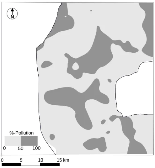
chemistry of ca. 40% of the water samples (cf. %–Pollution values in column 18 of Appendix A); (4) These polluted samples are distributed by large areas within the studied region (Figure 2).

Results of the SiB Algorithm

The SiB algorithm explained the chemistry of 93 out of the 138 groundwater samples (67%). The conceptual weathering model, required for the algorithm to work, was set taking into account the mineralogical assemblage of Table 1: (a) plagioclase weathers to montmorillonite; (b) K-feldspar weathers to mixtures of illite plus vermiculite (rich in illite); (c) calcite and dolomite dissolve congruently. The specific compositions of most minerals were not known and therefore, in order to write the weathering reactions (Table 2a), some educated guesses about those compositions had to be made (Table 2b). The best-fit solutions are shown in Table 3 (sample numbers in column 1). The predicted clay mineral abundances are listed in columns 2–4 and on average are: [Ca-montmorillonite] = 19%, [Illite] = 14% and [Vermiculite] = 1%. These numbers agree with the observed clay mineral abundances (Table 1), meaning that our results are realistic.

The best-fit plagioclase compositions are listed in column 5 of Table 3 and on average An = 0.5. The SiB model allowed K-feldspar to produce mixtures of illite and vermiculite, but in the vast majority of cases (83%) the best-fit reactions produced the end-member illite. The best-fit weathering reactions of K-feldspar are listed in column 6. If, for example, cK-spar = 40, hydrolysis of K-feldspar is represented by the symbolic reaction K-feldspar  0.4Illite + 0.6Vermiculite. The mass transfers of plagioclase, K-feldspar, calcite and dolomite are depicted in columns 7–10. On average, these transfers are put on the sequence [dolomite] (1447 mol/l) > [calcite] (708) > [plagioclase] (648) > [K-feldspar] (157), which is in fair agreement with widely accepted sequences of mineral weatherability, except for the position of calcite that frequently is the first mineral in the row (the most weatherable). For example, in Drever and Clow (1995) the

dissolution rate of calcite is reported to be 16.7 times faster than the rate of dolomite. We believe the exchange of positions between calcite and dolomite could be attributed to calcite

precipitation, for example in the course of “dedolomitization reactions” driven by effluent- and/or fertilizer-contaminated groundwaters rich in calcium.

Columns 11–14 describe the concentrations of cations that could not be assigned to weathering reactions. In total they match the concentrations of chloride + sulfate + nitrate and on average are dominated in equal proportions by magnesium and calcium ([Mg]p=1060 and [Ca]p=1029 mol/l). A bit less important is the anthropogenic contribution of sodium ([Na]p = 923 mol/l), and the less important of all man-controlled inputs is of potassium ([K]p = 249 mol/l).

Geochemical Patterns Supporting “Dedolomitization Reactions”

An important portion of the groundwater samples (95, representing approximately 70% of the dataset) are simultaneously supersaturated or close to equilibrium with respect to calcite (they are above the SI limit of 0.5 from equilibrium), undersaturated or close to equilibrium with respect to dolomite (they are below the SI limit of +0.5 from equilibrium), and undersaturated with respect to gypsum (Figure 3; individual saturation indices depicted in the last three columns of Appendix A). Put another way, these samples satisfy the thermodynamic prerequisites for the occurrence of “dedolomitization reactions”. The incidence of these reactions is also supported by the samples’ [Ca2+]/[SO42] and [Mg2+]/[SO42] ratios, as explained below.

The state of equilibrium between groundwater and the minerals calcite and dolomite is described by the following reaction:

Ca2+ + CaMg(CO3)2  2CaCO3 + Mg2+ (9)





 

When some oversaturation is observed with respect to calcite (present case), the [Mg2+]/[Ca2+] is instead forced to:





 

where 0.4 is the median SIcc of the 95 groundwater samples. The dedolomitization reaction under

these circumstances is described by the reaction:

1.8CaSO4 + 0.8CaMg(CO3)2  1.6CaCO3 + Ca2+ + 0.8Mg2+ + 1.8SO42– (11) which forces the [Ca2+]/[SO42] ratio to 0.56 and the [Mg2+]/[SO42] ratio to 0.44. These ratios are found in our study area (Figures 4a,b). The ideal [Ca2+] vs. [SO42] and [Mg2+] vs. [SO42] trends are indicated by the dashed lines, and in both cases are closely followed by the actual fittings (solid lines). In view of these results we suggest that “dedolomitization reactions” are active in the Szigetvár loessy sediments. Recalling that ‘gypsum’-containing fertilizers are the sole source of CaSO4 in the area we also suggest that “dedolomitization reactions” are driven by anthropogenic activity.

The remaining 43 samples are either undersaturated with respect to calcite and dolomite (2 cases) or oversaturated with respect to both minerals (41 cases). In these cases ground waters are

actively dissolving carbonates, or else the CaSO4 inputs to the system result in precipitation of carbonate minerals.

CONCLUSIONS

The occurrence of “dedolomitization reactions” in the loess sediments of the Szigetvár area are deduced from thermodynamic patterns (SIcc  0.5, SIdol  0.5) and geochemical trends

([Ca2+]/[SO42] and [Mg2+]/[SO42] ratios compatible with the dedolomitization reaction).

Further, they are supported by a switch between calcite and dolomite in the weather sequence, as concluded by mass balance modeling. Given the fact that gypsum was not recognized in the local sediments and that ground waters contain large amounts of anthropogenic calcium and sulfate, it is suggested that dedolomitization is driven by percolation of these contaminated waters through the loess aquifer.

ACKNOWLEDGMENTS

The present study was funded by the project “Geochemical Inspection of Groundwaters”, theme “Shallow Groundwater State in South Somogy and Baranya”, of the Geological Institute of Hungary. We are grateful to the anonymous reviewers for their constructive suggestions and remarks, which helped improving the quality of our work.

APPENDIX A – THE SZIGETVÁR AREA DATASET

Symbols: Nr. – groundwater sample identification code; Date – date of sample collection; X, Y

and Z – coordinates of location; Neighbourhood – location relative to the villages (1 – outside the villages and distant from any house; 2 – close to a couple of houses remote from the villages; 3 – inside the villages); [Y] – concentration of dissolved component Y; ICP-AES – Inductively Coupled Plasma Spectrometry; IC – Ion Chromatography; DCB (%) – deviation from charge balance as calculated by Equation 1; %P – %–Pollution parameter as calculated by Equation B2;

SIcc, SIdol and SIgyb – saturation indices of groundwater with respect to calcite, dolomite and

APPENDIX B  THE %POLLUTION OF A GROUNDWATER SAMPLE

Using the method of Correspondence Analysis, a set of original or X variables is transformed onto a set of factors or F variables. The relation between the F and X variables is set on the basis of a linear equation:

Fi = wi1X1 + wi2X2 + ... + wipXp (B1)

If the signs of factor loadings (wi coefficients) are equal the corresponding X variables are

correlated positively in Fi, otherwise they are correlated negatively in that factor. From the

observation of these "sympathies" and "antipathies" among signs of factor loadings, Equation B1 may be rewritten in forms that encompass some physical or chemical meaning. For factor one that usually explains a major proportion of the system variance (usually > 50%), Equation B1 can be recast into a percent pollution parameter:

100 x Pollution Weathering Pollution Pollution %    (B2) with,

 





 









where w1 is a F1 loading. Square brackets denote molar concentrations (of chloride, sulfate,

nitrate, bicarbonate and silica) in the groundwater sample. Samples with %–Pollution less than 50% have weathering-dominated water chemistries and samples with %–Pollution greater than 50% have pollution-dominated water chemistries.

APPENDIX C – THE SIB MODEL

The SiB algorithm has been developed by Pacheco and Van der Weijden (1996) and extended by Pacheco et al. (1999), Pacheco and Van der Weijden (2002), Van der Weijden and Pacheco (2003) and Pacheco and Alencoão (2005). The model comprehends a set of mole balance and charge balance equations given by:

Mole balance equations –

 

   

q j ij  



Charge balance equation – z

 

 



  



 q, n and m are the number of primary minerals involved in the weathering process

(plagioclase, K-feldspar, calcite and dolomite in the present case), the number of

dissolved inorganic compounds that usually are released from the weathering reactions of minerals (in total six compounds – Na+, K+, Mg2+, Ca2+, HCO3– and H4SiO4), and the number of the latter compounds that usually are also derived from pollution (the four major cations);

 t and p mean total and derived from pollution, respectively;

 X represents a dissolved compound;

 M represents a mineral;

 Cl–, SO42– and NO3– are the abbreviations for chloride, sulfate and nitrate, the major

dissolved anions assumed to represent exclusively anthropogenic plus atmospheric inputs;

 Square brackets ([]) denote number of moles of a dissolved compound or a dissolved/precipitated mineral;

 ij is the ratio between the stoichiometric coefficients of dissolved compound i and

mineral j as retrieved from the weathering reaction of mineral j;

 ij[Mj]=[Xi]rj, where [Xi]rj is the number of moles of dissolved compound i derived from

reaction of Mj moles of mineral j;

 zk is the charge of cation k;

The number of equations in set C1,2 is seven. The unknowns of the system are the [M] and the [X]p variables, in total q+m. The SiB algorithm uses the Singular Value Decomposition

procedure as described in Press et al. (1989) to solve the set of equations because this procedure can handle efficiently (through least squares or minimizing procedures) the cases where the set is undetermined (q+m > 7) or overdetermined (q+m < 7). In the present case, set 1a,b is

undetermined.

The stoichiometric coefficients () are defined by the weathering reactions of the primary minerals. The SiB model has the ability to handle the cases where weathering of these minerals produces mixtures of minerals (e.g. a reaction of K-feldspar to a mixture of illite plus

vermiculite). In this context, it includes an iterative or batch procedure whereby the weathering reactions produce solely end-members (e.g. illite or vermiculite) or else mixtures in pre-defined proportions (e.g. 90% illite plus 10% vermiculite). The SiB algorithm has also an additional loop procedure to handle cases of variable primary mineral composition (e.g. plagioclase varying in composition from An30 to An60). The [X]r are called constrained concentrations because they must fit into the stoichiometric relations of the mineral weathering reactions ([X]r[M]) but the SiB algorithm provides the flexibility to deal with situations where not all contributions to

groundwater chemistry are stoichiometrically constrained. This flexibility is gained through the inclusion of an unconstrained term in the mole balance equations – the [X]p term in the left-hand side of Equation C1.

Not all reactions tested by the SiB algorithm’s loop procedures explain the chemical

compositions of the groundwaters. To be labelled as a possible solution the set of weathering reactions must give [M] ≥ 0 and [X]p ≥ 0, except for minerals such as calcite or dolomite for which dissolution ([M] > 0) as well precipitation ([M] < 0) are allowed. If precipitation of these minerals has followed an initial stage of dissolution by meteoric water, then [M] = [M]dissolved 

[M]precipitated. However, with the SiB algorithm, only the net contribution ([M]) is assessed.

Among the possible solutions, the SiB algorithm selects a best-fit one by testing all sets against predefined external boundary conditions, the most common being the clay-test whereby

abundances of secondary products as predicted by the algorithm are compared with abundances present in the aquifer material. The theoretical clay mineral abundances (predicted by the SiB model) are determined as follows:

 

 

where l represents a weathering product derived from primary mineral j and lj is the rate at

which product l is being formed as a consequence of the rate at which mineral j is being weathered. Subscript l is restricted to the value of 1 if mineral j produces a single weathering product or to the values of 1 or 2 if mixtures of secondary minerals are allowed for that primary mineral. In the present study, the clay-test was used as external boundary condition. To be considered a best-fit solution, the predicted abundances of secondary minerals should approach as much as possible [Montmorillonite] = 20.4%, [Illite] = 11% and [Vermiculite] = 2%, in agreement with the values shown in Table 1.

REFERENCES

Alonso-Zarza, A.M., Sanchez-Moya, Y., Bustillo, M.A., Sopena, A., Delgado, A., 2002. Silicification and dolomitization of anhydrite nodules in argillaceous terrestrial deposits: an example of meteoric-dominated diagenesis from the Triassic of central Spain. Sedimentology 49, 303–317.

Appelo, C.A.J., Postma, D., 1993. Geochemistry, groundwater and pollution. Balkema, Rotterdam, 535p.

Arenas, C., Zarza, A.M.A., Pardo, G., 1999. Dedolomitization and other early diagenetic

processes in Miocene lacustrine deposits, Ebro Basin (Spain). Sedimentary Geology 125, 23–45.

Ayora, C., Taberner, C., Saaltink, M.W., Carrera, J., 1998. The genesis of dedolomites: a discussion based on reactive transport modelling. Journal of Hydrology 209, 346–365.

Bischoff, J.L., Julia R., Shanks, W.C., Rosenbauer, R.J., 1994. Karstification without carbonic acid. Bedrock dissolution by gypsum-driven dedolomitization. Geology 22, 995–998.

Blatt, H., 1992. Sedimentary petrology (2nd ed.). W.H. Freeman and Company, New York, 514p.

Canaveras, J.C., SanchezMoral, S., Calvo, J.P., Hoyos, M., Ordonez, S., 1996. Dedolomites associated with karstification. An example of early dedolomitization in lacustrine sequences from the tertiary Madrid basin, central Spain. Carbonates and Evaporites 11, 85–103.

Capaccioni, B., Didero, M., Paletta, C., Salvadori, P, 2001. Hydrogeochemistry of groundwaters from carbonate formations with basal gypsiferous layers: an example from the Mt Catria Mt Nerone ridge (Northern Appennines, Italy). Journal of Hydrology 253, 14–26.

Capo, R.C., Whipkey, C.E., Blachere, J., Chadwick, O.A., 2000. Pedogenic origin of dolomite in a basaltic weathering profile, Kohala, Peninsula, Hawaii. Geology 28, 271–274.

Drever, J.I., Clow, D.W., 1995. Weathering rates in catchments. In: A.F. White & S.L. Brantley (Eds.) Chemical Weathering Rates of Silicate Minerals. Reviews in Mineralogy, Volume 31, Mineralogical Society of America, Washington D.C., USA., p. 463–483.

Goldstrand, P.M., Shevenell, L.A., 1997. Geologic controls on porosity development in the Maynardville limestone, Oak Ridge, Tennessee. Environmental Geology 31, 248–258.

Guo, B.Y., Sanders, J.E., Friedman, G.M., 1996. Timing and origin of dedolomite in upper Wappinger Group (lower Ordovician) strata, southeastern New York. Carbonates and Evaporites 11, 113–133.

James N.P., Bone, Y., Kyser, TK, 1993. Shallow burial dolomitization and dedolomitization of mid-Cenozoic, cool-water, calcitic, deep-shelf limestones. Journal of Sedimentary Petrology 63, 528–538.

Kargel, J.S., Schreiber, J.F., Sonett, C.P., 1996. Mud cracks and dedolomitization in the Wittenoom Dolomite, Hamersley Group, Western Australia. Global and Planetary Change 14, 73–96.

Khalaf, F.I., Abdal, M.S., 1993. Dedolomitization of dolocrete deposits in Kuwait, Arabian Gulf. Geologische Rundschau 82, 741–749.

Kenny, R., 1992. Origin of disconformity dedolomite in the martin formation (late Devonian, northern Arizona). Sedimentary Geology 78, 137–146.

Kolkas, M.M., Friedman, G.M., 1998. Diagenetic history and geochemistry of the Beekmantown-Group dolomites (Sauk sequence) of New York, USA. Carbonates and Evaporites 13, 69–85.

López-Chicano, M., Bouamama, M., Vallejos, A., Pulido-Bosch, A., 2001. Factors which determine the hydrogeochemical behaviour of karstic springs. A case study from the Betic Cordilleras, Spain. Applied Geochemistry 16, 1179–1192.

Masaryk, P., Lintnerova, O., 1997. Diagenesis and porosity of the Upper Triassic carbonates of the pre-Neogene Vienna Basin basement. Geologica Carpathica 48, 371–386.

Pacheco, F.A.L., 1998. Application of Correspondence Analysis in the assessment of groundwater chemistry. Mathematical Geology 30, 129–161.

Pacheco, F.A.L., Alencoão, A.M.P., 2005. Role of fractures in weathering of solid rocks:

narrowing the gap between experimental and natural weathering rates? Journal of Hydrology (in press article).

Pacheco, F.A.L., Landim, P.M.B, 2005. Two-way regionalized classification of multivariate data sets and its application to the assessment of hydrodynamic dispersion. Mathematical Geology 37(4), 393417.

Pacheco, F.A.L., Sousa Oliveira, A., Van der Weijden, A.J., Van der Weijden, C.H., 1999. Weathering, biomass production and groundwater chemistry in an area of dominant

anthropogenic influence, the Chaves-Vila Pouca de Aguiar region, north of Portugal. Water, Air and Soil Pollution 115, 481–512.

Pacheco, F.A.L., Van der Weijden, C. H., 1996. Contributions of Water-Rock Interactions to the Composition of Groundwater in Areas With Sizeable Anthropogenic Input. A Case Study of the Waters of the Fundão Area, Central Portugal. Water Resources Research 32, 3553–3570.

Pacheco, F.A.L., Van der Weijden, C. H., 2002. Mineral weathering rates calculated from spring water data: a case study in an area with intensive agriculture, the Morais Massif, NE Portugal. Applied Geochemistry 17, 583–603.

Perry, E., Velazquez-Oliman, G., Marin, L., 2002. The hydrogeochemistry of the karst aquifer system of the northern Yucatan Peninsula, Mexico. International Geology Review 44, 191–221.

Peryt, T.M., Scholle, P.A., 1996. Regional setting and role of meteoric water in dolomite formation and diagenesis in an evaporite basin: studies in the Zechstein (Permian) deposits of Poland. Sedimentology 43, 1005–1023.

Plummer, L.N., Busby, J.F., Lee, R. W., et al., 1990. Geochemical modeling of the Madison aquifer in parts of Montana, Wyoming, and South Dakota. Water Resources Research 26, 1981– 2014.

Press, W.H., Flannery, B.P., Teukolsky, S.A., Vetterling, W.T., 1989. Numerical recipes in Pascal, Cambridge University Press, Cambridge.

Qian, G.R., Deng, M., Tang, M.S., 2002. Expansion of siliceous and dolomitic aggregates in lithium hydroxide solution. Cement and Concrete Research 32, 763–768.

Raines, M.A., Dewers, T.A., 1997. Dedolomitization as a driving mechanism for karst generation in Permian Blaine formation, southwestern Oklahoma, USA. Carbonates and Evaporites 12, 24–31.

Sacks, L.A., Herman, J.S., Kauffman, S.J., 1995. Controls on high sulfate concentrations in the Upper Floridan Aquifer in Southwest Florida. Water Resources Research 31, 2541–2551.

Sanz-Rubio, E., Sanchez-Moral, S., Canaveras, J.C., Calvo, J.P., Rouchy, J.M., 2001. Calcitization of Mg-Ca carbonate and Ca sulfate deposits in a continental Tertiary basin (Calatayud Basin, NE Spain). Sedimentary Geology 140, 123–142.

Singurindy, O., Berkowitz, B., 2003. Flow, dissolution and precipitation in dolomite. Water Resources Research 39, 1143–1143.

Spry, P.G., Cody, R.D., Cody, A.M., Spry, P.G., 2002. Observations on brucite formation and the role of brucite in Iowa highway concrete deterioration. Environmental & Engineering Geoscience 8, 137–145.

Stumm, W., Morgan, J. (1996). Aquatic Chemistry. John Wiley and Sons Inc., New York etc., 1022 p.

Van der Weijden, C.H., Pacheco, F.A.L., 2003. Hydrochemistry, weathering and weathering rates on Madeira island. Journal of Hydrology 283, 122–145.

Wang, Y., Ma, T., Luo, Z., 2001. Geostatistical and geochemical analysis of surface water leakage into groundwater on a regional scale: a case study in the Liulin karst system, northwestern China. Journal of Hydrology 246, 223–234.

Zeeh, S., Becker, F., Heggemann, H., 2000. Dedolomitization by meteoric fluids: the Korbach fissure of the Hessian Zechstein basin, Germany. Journal of Geochemical Exploration 69, 173– 176.

TABLE LEGENDS

Table 1 – Mineralogical composition of loess, determined by RTG. Discussion of the RTG analyses in the proper analytical section.

Table 2a – List of weathering reactions used in the mole balance calculations (SiB model; Pacheco and Van der Weijden, 1996). The reactants are plagioclase, K-feldspar, calcite and dolomite. The secondary products are Ca-montmorillonite, vermiculite and illite. The assumed chemical compositions of the minerals are given in Table 2b.

Table 2b – Assumed chemical compositions of the minerals involved in the weathering reactions.

x is the anorthite content of plagioclase and varies in the range 0.3 < x < 0.6.

FIGURE CAPTIONS

Figure 1a – Location and geological sketch of the Szigetvár area. Location of the sampling sites (loess area).

Figure 1b – Topography, drainage pattern and location of villages inside the loess area.

Figure 2  Spatial distribution of areas with weathering-dominated water chemistries and areas with pollution-dominated water chemistries, as drawn on the basis of a method hinged on Correspondence Analysis, developed by Pacheco (1998).

Figure 3 – Comparison of calcite, dolomite and gypsum saturation indices as a function of total dissolved sulfate, in the 95 groundwater samples that are simultaneously supersaturated (or in equilibrium) with respect to calcite, undersaturated (or in equilibrium) with respect to dolomite and undersaturated with respect to gypsum. Saturation indices of all samples are listed in the last three columns of Appendix A.

Figure 4 – Comparison of concentrations of (a) dissolved calcium and (b) magnesium as a function of dissolved sulfate. Solid lines are fittings to measured values whereas dashed lines indicate the expected trends when groundwater is supersaturated for calcite (median SIcc = 0.4).

TABLE 1 Mineral Abundance (wt%) Quartz 37 K-feldspar 3 Plagioclase 8.4 Mica 1.2 Amphibolite 0.4 Vermiculite 2 Montmorillonite 20.4 Illite 11 Kaolinite 2 Chlorite 3 Calcite 6.8 Dolomite 3.9

TABLE 2a

Primary Mineral

Secondary Product Reaction (round off coefficients)

Plagioclase (Pl) Ca-montmorillonite (Ca-m) -3 3 2 2 2 2 HSiO 2HCO 1 6 3.32 Ca 1 167 . 0 2.167 Na 1 1 2.33 m Ca 2CO O H Pl 1 2.33 _                                   x x x x x x n x K-Feldspar (K-sp) Vermiculite (Vm)

1.5K-sp + nH2O + 0.7Mg2+ + 0.8HCO3- → Vm + 0.6K+ + 0.7H4SiO4 + 0.8CO2

K-Feldspar (K-sp)

Illite (Il)

2.3K-sp + nH2O + 0.25Mg2+ + 1.25CO2 → Il + 1.75K+ + 3.45 H4SiO4 + 1.25HCO3–

Calcite (Cc) Cc + H2O + CO2 → Ca2+ + 2HCO3– Dolomite (Dol) Dol + 2H2O + 2CO2 → Mg 2+ + Ca2+ + 4HCO3–

TABLE 2b

Mineral Structural formula

Plagioclase Na1–x CaxAl1+x Si3–xO8

K-feldspar KAlSi3O8 Calcite CaCO3 Dolomite CaMg(CO3)2 Ca-montmorillonite Ca0.167Al2.33Si3.67O10(OH)2 Vermiculite K0.9(Al1.3Mg0.7)(Si3.8Al0.2)O10(OH)2 Illite K0.55(Al1.75Mg0.25)(Si3.45Al0.55)O10(OH)2

FIGURE 1a

1 to 2 2 to 3 3 to 3.001

FIGURE 1b 100 140 180 220 260 300 340 Height (m) N 0 500 1000 1500 0 5 10 15 km Village Stream

FIGURE 2 0 500 1000 1500 0 5 10 15 km 0 50 100 %-Pollution 0 50 100 N

FIGURE 3 -3.0 -2.5 -2.0 -1.5 -1.0 -0.5 0.0 0.5 1.0 0.0 0.5 1.0 1.5 2.0 2.5 3.0 3.5 4.0 [SO4 2-] (mmol/l) SI Calcite Dolomite Gypsum

FIGURE 4

(a) [SO42] vs. [Ca2+]

0.0 1.0 2.0 3.0 4.0 5.0 6.0 7.0 8.0 0.0 0.5 1.0 1.5 2.0 2.5 3.0 3.5 4.0 [SO4 2-] (mmol/l) [Ca 2+ ] (mmo l/ l) Measured values Theoretical fitting Observed fitting (a) (b) [SO42] vs. [Mg2+] 0.0 1.0 2.0 3.0 4.0 5.0 6.0 7.0 8.0 9.0 10.0 0.0 0.5 1.0 1.5 2.0 2.5 3.0 3.5 4.0 [SO4 2-] (mmol/l) [Mg 2+ ] (mm ol /l ) Measured values Theoretical fitting Observed fitting (b)