Changing Perspectives: Interlead Conversion in Electrocardiographic Signals

Changing Perspectives: Interlead

Conversion in Electrocardiographic

Signals

Departamento de Ciˆ

encia de Computadores

Faculdade de Ciˆ

encias da Universidade do Porto

Changing Perspectives: Interlead

Conversion in Electrocardiographic

Signals

Dissertation

Supervisor: Miguel Tavares Coimbra Co-supervisor: Jo˜ao Tiago Ribeiro Pinto

Departamento de Ciˆencia de Computadores Faculdade de Ciˆencias da Universidade do Porto

want to thank Jo˜ao Ribeiro Pinto, for always guiding me in the best way, helping me to evolve, and always wanting to go further. To professor Miguel Coimbra, for showing me the area of computer vision and making

me choose it as the basis for the development of my work. Second, I thank my parents who always supported me during these years of college.

Finally to all my friends who were with me during this stage and to the Faculdade de Ciˆencias that was my second home during these years.

The electrocardiogram (ECG) is a physiological signal that measures the conduction of electrical currents through the heart, that allow for its contraction and relaxation to maintain adequate blood flow[3]. In the standard configuration, widely used in medical settings for heart monitoring and diagnosis, the ECG is acquired using elec-trodes in contact with the subject’s wrists, ankles, and chest. When connecting two electrodes, we get a view of the heart, named Lead. In this dissertation, we studied how to convert those Leads into others, with the goal of helping with the diagnosis of some heart diseases by predicting the Leads that are missing from the recordings without having to submit the patient to various exams. For this task, we relied on signal processing and machine learning techniques with special focus on robust deep learning architectures, such as autoencoders, and implemented an algorithm that can be adaptable for the conversion into other Leads. This work paves the way towards easier and more comfortable ECG exams without losing potential for diagnosis - one Lead will be sufficient as the algorithm is able to accurately convert it into all other heart perspectives.

Abstract 4 List of Tables 8 List of Figures 11 1 Introduction 12 1.1 Motivation . . . 12 1.2 Objectives . . . 13 1.3 Contribution . . . 14 1.4 Thesis Structure . . . 15 2 Background 17 2.1 Biosignals . . . 18 2.1.1 Electrocardiogram (ECG) . . . 19 2.1.2 Signal processing . . . 21 2.2 Machine Learning . . . 22 2.3 Deep Learning . . . 24 2.3.1 Autoencoders . . . 25

2.3.2 Convolution neural network (CNN) . . . 30

2.3.3 Keras and Tensorflow . . . 31

3 Related Work 34

3.1 Conversion of ECG Leads . . . 34

3.2 Conversion of ECG Graph into Digital Format . . . 36

3.3 Deepfakes . . . 37

4 Methodology 41 4.1 Materials . . . 41

4.2 Pre-processing . . . 42

4.3 Fully connected autoencoder . . . 42

4.4 Convolutional autoencoder . . . 43

4.5 Autoencoder . . . 44

4.5.1 Fully-connected . . . 44

4.5.2 Fully connected multi-output . . . 45

4.5.3 Convolutional autoencoder . . . 46

4.5.4 Convolutional autoencoder multi-output . . . 47

5 Experimental Methodology 49 5.1 General approach of the autoencoders . . . 49

5.2 Evaluation metrics . . . 57

5.3 Our approach to the analysis of the results . . . 58

6 Results 59 6.1 Qualitative Results . . . 59

6.1.1 Prediction of the same Lead . . . 60

6.1.2 Conversion to Lead I . . . 61

6.1.4 Conversion/Prediction of leads using a convolutional autoencoder 64

6.1.5 Conversion convolutional autoencoder multi-output . . . 66

6.2 Quantitative results . . . 67

7 Discussion 75

8 Conclusion 77

References 79

6.1 Analysis of the different metrics in a 11 layer fully-connected autoencoder 68

6.2 Analysis of the different metrics in a 9 layer fully-connected autoencoder 68

6.3 Analysis of the different metrics in a 7 layer fully-connected autoencoder 69

6.4 Analysis of the different metrics in fully-connected multi-output au-toencoder . . . 72

6.5 Analysis of the different metrics in a convolutional autoencoder . . . . 73

1.1 General architecture of our algorithm - diagram . . . 14

1.2 Standard 12-Lead configuration . . . 15

2.1 ECG record . . . 18

2.2 EMG record . . . 18

2.3 EEG record . . . 18

2.4 EOG record . . . 18

2.5 Representation of the fiducial landmarks in a heartbeat . . . 20

2.6 General architecture of an autoencoder . . . 26

2.7 Representation of the different parts that make an autoencoder . . . . 26

2.8 Example of the autoencoder with the mnist database . . . 27

3.1 Representation of the phases of the autoencoder . . . 38

3.2 Representation of two different autoencoders that will focus on different features . . . 39

3.3 Autoencoder deepfake creation scheme . . . 40

4.1 Autoencoder multi-output architecture . . . 45

4.2 Representation of the UNet general architecture . . . 46

4.3 Representation of the contracting path in the Unet . . . 47

4.4 Representation of the expansive path in the Unet . . . 47

5.2 Conversion autoencoder architecture . . . 50

5.3 Conversion Lead I → Lead I . . . 51

5.4 Conversion Lead II → Lead I . . . 51

5.5 Conversion Lead III → Lead I . . . 52

5.6 Conversion autoencoder multi-output architecture . . . 52

5.7 Conversion xtrain → Lead I . . . 53

5.8 Conversion xtrain → Lead II . . . 53

5.9 Conversion xtrain → Lead III . . . 53

5.10 Convolution autoencoder architecture . . . 54

5.11 Conversion Lead I → Lead I . . . 55

5.12 Convolution multi-output autoencoder architecture . . . 56

5.13 Conversion convolutional xtrain → Lead I . . . 57

5.14 Conversion convolutional xtrain → Lead II . . . 57

5.15 Conversion convolutional xtrain → Lead III . . . 57

6.1 Prediction Lead I → Lead I . . . 60

6.2 Prediction Lead II → Lead II . . . 60

6.3 Prediction Lead III → Lead III . . . 60

6.4 Target Lead representation - Lead I . . . 62

6.5 Conversion Lead II → Lead I . . . 62

6.6 Conversion Lead III → Lead I . . . 62

6.7 Conversion xtrain → Lead I . . . 63

6.8 Conversion xtrain → Lead II . . . 64

6.9 Conversion xtrain → Lead III . . . 64

6.10 Prediction Lead I → Lead I . . . 65

6.12 Conversion Lead III → Lead I . . . 65

6.13 Prediction LeadI . . . 66

6.14 Conversion LeadII . . . 66

6.15 Conversion LeadIII . . . 66

Introduction

After research on Lead conversion on electrocardiograms (ECG), we concluded that there was no great progress in the idea that we came to propose in this thesis. A normal electrocardiogram consists of a recording of 12 Leads, and what we are going to see is the implementation of an algorithm that allows us to convert these Leads into each other. “What is the purpose of this idea?”, “what is its contribution to medicine?”, “is it necessary to have the possibility of this conversion?”, “what is its use?”. So many questions that came to us but that also served as motivation for this implementation. In this section we will introduce our idea, explaining our motivation, objectives, contributions, and finally defining the structure of the thesis.

1.1

Motivation

The electrocardiogram (ECG) is a physiological signal that measures the conduction of electrical currents through the heart, that allows for its contraction and relaxation to maintain adequate blood flow[3]. In the standard configuration, widely used in medical settings for heart monitoring and diagnosis is acquired using electrodes in contact with the subject’s wrists, ankles, and chest.

Depending on the location of the electrodes, the electrocardiogram offers a different perspective of the heart. Hence, the usefulness of each Lead depends on the expected application. In biometrics, the most commonly used channel is Lead I (right arm -left arm) for improved usability and user comfort.

In healthcare, each Lead offers insight into specific conditions or irregularities.

ever, in several cases, the most favorable Lead may be unavailable, and professionals(or automatic systems) may be forced to use less adequate Leads.

Despite ECG in machine learning is usually used for arrhythmia detection, in this thesis, we will focus the use of ECGs as a biosignal for the development of methods for automatic conversion of Leads in electrocardiograph signals, which will help in the diagnose of some heart diseases, without having to submit the patient to various exams.

As a result of this thesis, it is expected to have an algorithm to convert, as faithfully as possible, ECG signals from certain Leads into target Leads, being this targets the Leads we need depending on the task. This will be achieved by resorting to signal processing and machine learning techniques, with a special focus on robust deep learning architectures.

Focusing on biometric applications, and the development of our work we are mainly going to have as the conversion target the Lead I, due to its acquisition being more accepted since the electrodes are positioned on the wrists[27], but the algorithm is expected to be adaptable for the conversion into other Leads.

1.2

Objectives

The big question we want to see answered in this thesis is, “is it possible?”. All this uncertainty that comes together when we start research on a topic in an almost pioneering way, that is, when we do not find large studies on what we want to have some ideas that support our decisions, it always gives that additional motivation to continue and prove that we will achieve something. Thinking now in a more scientific way, what we want is to realize if the conversion of Leads is possible, so that, the information given by each one of them is not lost.

To forward our thesis so that we can get these answers, we organize our tasks as follows:

• Prior art study: bibliography review on ECG acquisition, Leads, datasets; • Define the experimental protocol;

• Prepare data;

• Design and implementation of the conversion model; • Training of the implemented model;

• Evaluate performance and compare with the state-of-the-art;

1.3

Contribution

The contributing factor behind the implementation of this new conversion system is purely to be in par with changing technology and to enhance the existing deep learning techniques that are efficient. Resulting in higher quality and accuracy.

Our approach to this problem, consists in the creation of an algorithm to convert ECG signals from certain Leads, into a target one and the way we are planning to tackle this problem is by implementing an autoencoder that will have as an input the Lead to convert, code it an decode it into another Lead. If we can develop this idea and have good results, we also aim to extend this conversion so that instead of having only one target, we will have several.

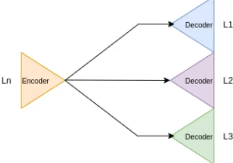
The next image shows, the architecture we design for our algorithm:

Figure 1.1: General architecture of our algorithm - diagram

As we can see in the diagram above that shows the idea of our algorithm. What we plan to do is to create autoencoders that take a Lead and rebuild it, and then combine the encoders of the different Leads with a decoder that will convert to the Lead I. What we want with this creation of an autoencoder per Lead is that the respective encoder will be able to create coding for each one of them so that when we go to the decoder it will be able to find the correlations and thus convert into another.

Understanding all different Leads, and the way an autoencoder works is a key factor for successful results. Therefore before we proceed to explain the objectives for this work,

the first thing to clarify is the definition of the word “Lead” in the ECG context. A Lead refers to an imaginary line between two ECG electrodes.[29] The electrical activity of this Lead is measured and recorded as part of the ECG. The 12 Leads are made up of three bipolar and nine monopolar Leads. The three bipolar Leads are the electrical potentials between the right and left arm (Lead I), the right arm and left foot (Lead II), and between the left arm and left foot (Lead III). For the monopolar Leads, four different artificial reference points are constructed. Using these reference points, the potentials appearing on the left arm (VL), the right arm (VR), the left foot (VF), and on the six chest electrodes (V1-V6) are measured.[3]

Figure 1.2: Standard 12-Lead configuration[27]

This will pave the way towards the obsolescence of laborious and uncomfortable multi-Lead ECG exams - one multi-Lead will be sufficient as the algorithm would be able to accurately convert it into all other heart perspectives.

1.4

Thesis Structure

This thesis is organized as follows: we have eight chapters, Background (chapter 2), in this chapter we described every tool, concept and techniques we use during the development task, Related work (chapter 3), in here we describe all the related work we found regarding what we needed for the thesis, but mainly this chapter is used as an introduction for the basic concepts we need to be familiarized with before

start the implementation, Methodology (chapter 4), in here we describe all the work done, Experimental Methodology (chapter 5), where we explain everything that is useful to give a better understanding of the methods, Results (chapter 6) where we show and explain all the results in a quantitative and qualitative approach and give some lights on improvements that we think it can be done, Discussion (chapter 7), here we discuss everything that can be improved and done as future work having as basis our model, and the last one, Conclusion (chapter 9), where we do a recap of the all thesis explaining the strongest and weakest points that we have at this point, with the hope this first approach to this theme will help and attract more research to this field.

Background

As mention in the previous section, the goal of this thesis is the implementation of a Lead convert algorithm, that is adaptable to convert any kind of Lead. Before begin-ning this implementation it is important to understand all the techniques, methods, terms, and everything else related to this topic, and that’s why this chapter exists. In this section, we are going to explain in detail all these things, to help understand our algorithm and its purpose.

In a theoretical approach, our algorithm is going to have four steps: data normaliza-tion, encoder, decoder, and evaluation. In the first step, we are going to make sure that all the data (electrocardiogram (ECG) signals) have the same properties, such as size, find the location of its peaks, and are all center in the same peak. When we get to the encoder part, here we are already in the autoencoder, and we are expecting that the signal is being learned, to guarantee that in the next phase (decoder) the signal is reconstructed as accurately as possible. For the last step, we are going to apply metrics to verify the accuracy of the reconstruction.

Before we start explaining what are autoencoders and how they work, we are going to start explaining some terms, that are the key for the understanding, not only our algorithm but also the motivation that led us to try and create it. When we started our research on this topic we realized quickly that not a lot of work has been done in this kind of conversion, and so that was one of the main reasons that make us interested in trying it.

Since the main focus of this thesis is signal processing, one of the terms that we must know is biological signals because we are working with ECGs, as well as the signal pro-cessing techniques themselves to be able to understand further on the transformations

that were made to the ECG signal.

2.1

Biosignals

A biosignal is any signal in human beings that can be continually measured and monitored like electrocardiogram (ECG) from the heart, electromyogram (EMG) from the muscles, electroencephalogram (EEG) from the brain and electrooculogram (EOG) from the eyes, among others.[8]

The practical applications for biosignals are associated with the monitoring of physical activity. In medicine, they are used to test resistance to physical activity[8], how we will see it later on, when we talk about ECGs and how they are recorded.

Figure 2.1: ECG record[11] Figure 2.2: EMG record[30]

Figure 2.3: EEG record[21] Figure 2.4: EOG record[31]

The biosignals can be continuous (x(t)), discrete (x(n), where n = 0,1,2,3...), deter-ministic and random. Continuous signals can be defined over continuous values of time and space. Discrete signals define only a subset of regularly spaced points in time, continuous signals from the human body are converted to discrete signals by a process called sampling and they can be analyzed and interpreted by a computer.[10]

Deter-ministic biosignals can be described by mathematical functions or rules, it illustrates the initial conditions. Deterministic processes can be divided into:

• Transitional processes - action system measured biosignals that are recorded only once.

• Established processes - the system will vary periodically in time or does not change at all.

A periodic signal is a good example of a deterministic biosignal, x(t) = x(t + nT ), repeats itself every T units in time, so T represents the period. The other kind of biosignal is random, and we can divide this type into random stochastic signals, that contain uncertainty in the parameters that describe them, so it cannot be precisely described by mathematical functions, it is often analyzed using statistical techniques with probability distributions or simple statistical measures such as the mean and standard deviation, and stationary random signals, where the statistics or frequency spectra of the signal remain constant over time.[10]

2.1.1

Electrocardiogram (ECG)

Once we define a biosignal and since we are working with one in this thesis, we should understand what an ECG is, not only as a biosignal but what is used for, and with that being said, the ECG is an exam used for diagnosing, because it evaluates the heart function. Despite all the continuous evolution of technology, the ECG still holds the main role in the research of heart diseases, it consists of an exam that detects the electrical activity of the heart. Each contraction of the heart muscle is commanded by small electrical impulses that are generated by it. This set of electrical impulses generates a signal - the ECG -, and which is formed by a set of P, Q, R, S and T waves that are repeated over time.[27] The ECG can also identify normal transmission patterns and the generation of the electrical impulses. It has great value in the evaluation of some types of heart abnormalities, including heart valves diseases, cardiomyopathy, pericarditis, and cardiac squeals of hypertension. Being a harmless exam and inexpensive, it is most useful for the study of the heart.

There are three types of ECG, resting, stress, and the Holter exam: The resting is done with the patient lying down and with his bare torso. The ideal situation is that the patient before the exam made no effort in the past 10 minutes, and has not smoked in the past 30 minutes. The patient should also avoid drinking cold water

because it can change the signal. During the exam 10 electrodes are placed on the patient (6 on the chest, 2 on the wrist, and 2 placed on the ankles). The electrodes are wires that you attach to the patient to record the ECG. They allow Leads to be calculated. For regular ECG recordings, the variations in electrical potentials in 12 different directions (Leads) out of the ten electrodes are measured. After placing all the electrodes, they are connected to a machine that will perform the ECG. The exam only takes a couple of minutes, and during that time the machine records the electrical signals and draws them in a specific paper. The resting ECG is one of the most performed exams because it is cheap, fast, and easy to do. On the other hand, stress ECG requires another kind of equipment, like a treadmill or an exercise bike, which makes it more expensive. This exam allows the evaluation of the heart in stress conditions. If the resting ECG is normal and the history of the patient is suggestive of heart disease, the stress ECG can show alterations not before seen in the other. The Holter exam, in which it is recorded the heart activity during 24 hours, let us study the behavior of the heart during a day, comparing it with activities carried out and with the patient symptoms, that are recorded in a diary.[1]

The ECG tracing consists of 5 elements: wave P, interval PR, complex QRS, segment ST and wave T. The wave P corresponds to the depolarization of the auricle, the interval PR is the time since the beginning of the depolarization of the auricles and ventricles, the complex QRS corresponds to the depolarization of the ventricles, the segment ST is the time between the end of depolarization and the beginning of the repolarization of the ventricles and the wave T is the repolarization of the ventricles, that are ready to another contraction. Each heartbeat is made of a wave P, one complex QRS and one wave T.[20]

2.1.2

Signal processing

Signal processing is the analysis or modification of signals using fundamental theory, applications, and algorithms, to extract information from them in a way that makes them more suitable for specific applications. The processing can be done in an ana-logical or digital way. This process uses mathematics, statistics, computing, heuristics and linguistic representations, formalism and representation techniques, modeling, analysis, synthesis, discovery, recovery, detection, acquisition, extraction, learning, security, and forensics[23]. The sample for signal processing can include, sounds, images, temporal series, telecommunications signals, among others.

The techniques of signal processing can show great use in the analysis and control of physic systems of interest to the most diverse researchers, not only electrical engineers but mechanical engineers. Nowadays signal processing is being brought to the atten-tion of professionals in other fields of study like economy, biology, health, and they can integrate both health and computer technologies.

As we saw before, the fields to use signal processing are endless, so to get the same technique suitable for the different applications, we have different types of processing depending on the kind of signal we are dealing with, like the analogical signal, non-linear signal, discrete signal, and digital signal.

• Analogical signal: Any kind of processing used in analogical signals is done through analogical means. Analogical values are usually represented by tension, electric current, or electrical charge in electrical devices. Analogical signal processing is done in signals that have not been scanned yet, like radio, telephone and radar signals, television systems. This process involves electrical linear and non-linear circuits.

• Non-linear signal: Signal non-linear processing involves the analysis and pro-cessing of signals produced by non-linear systems and can be determined by time, frequency, or space-time domains[4].

• Discrete signal: Discrete signal is a temporal series that consists of a quantity sequence, a function on the discrete integer domain. Each value in the sequence is called a sample and is defined only in discrete points in time. Different from a continuous signal, a discrete one is not a function of a continuous argument. However, the function can be generated through a continuous signal of the sampling. We can obtain discrete signals in several ways, but normally they

are classified into two groups[18]. The first one is the acquisition of values of an analogical signal in time, a process called signal sampling. The second one is the accumulation of value in time, for example, the number of people that enter a room per day. The concept of discrete signal processing, establish a mathematical base for digital signal processing without quantization.

• Digital signal: The digital processing signal (DSP) is the mathematical ma-nipulation process of a signal, to modify it or improve it in some way. Is charac-terized through the discrete signal representation. It has several computational techniques that can be used directly in a computational system based on IBM-PC pattern, without needing to use specific hardware like FPGAs or micro-controllers. The Fourier transformations are one of the examples of this kind of processing. The goal of DSP is to measure, filter, and compress analogical signals. Usually, the first step for the conversion from analogical to digital is the sampling of the signal and then digitalize it using a converter analogical-digital, that transforms the analogical signal in a flow of digital discrete values. Often we need to have the conversion done oppositely, so a converter digital-analogical is also needed. The process of digital processing is more complex than the analogical signal processing, this application has a lot of computational power, which allows a lot of advantages, when comparing with the analogical signal processing in various applications, like detection and correction of errors in the transmission, as well as compression of data[6]. The DSP algorithms can be used in normal computers as well as computers that are specifically made for those types of processing. Nowadays, exists technologies used for signal processing like Field-programmable gate array (FPGA), digital signal controllers, among others.

2.2

Machine Learning

Machine learning (ML) is a sub-field of computer science engineers that evolved from the study of pattern recognition and the theory of machine learning in artificial intelligence. It explores the study and construction of algorithms that can learn from their mistakes and make predictions about data. Such algorithms operate by building a model from sample inputs to make predictions or decisions guided by the data rather than simply following inflexible and static programmed instructions. Whereas in artificial intelligence there are two types of reasoning, machine learning is only

concerned with inductive.[16]

When ML appeared, its goal was to make computers modify and adapt their actions according to the tasks they would have to perform. In this way and practical terms the ML algorithms “learn” the task to be able to perform it without errors, this is, with high accuracy.[22]

Some parts of machine learning are closely linked to computational statistics. They focus on how to make predictions through the use of computers, with research focusing on the properties of statistical methods and their computational complexity. It has strong ties to mathematical optimization, which produces methods, theory, and appli-cation domains for this field. Machine learning is used in a variety of computational tasks that work on creating and programming explicit algorithms that are impractical.

Machine learning is sometimes confused with data mining, which is a sub-field that focuses more on exploratory data analysis and is known as unsupervised learning. In the field of data analysis, machine learning is a method used to plan complex models and algorithms that lend themselves to make predictions, in commercial use, this is known as predictive analysis. These analytical models allow researchers, data scientists, engineers, and analysts to produce reliable and repeatable decisions, results and discover hidden insights by learning the historical relationships and trends in the data.[12]

Some types of machine learning[22]:

• Supervised learning - In this kind of learning, the algorithm analyses all the training data, and throughout that learning process it generates a function that will be used to map new examples.

• Unsupervised learning - The algorithm looks for patterns that were not detected yet and try to match with other inputs, when finds a match between two inputs, a category is created.

• Reinforcement learning - This one differs from supervised learning, once it does not need the training data, instead it tries to create a balance between exploratory (analyzing unknown patterns) and exploitation work.

2.3

Deep Learning

Deep learning is a type of machine learning, that trains computers to perform the task as humans, which includes voice recognition and image identification. Instead of organizing data to be trained through predefined equations, deep learning sets up basic parameters about data and trains the computer to learn by itself through patterns of recognition in many processing layers, based on a collective of algorithms that try to model high-level abstractions of data, using a deep graph with many layers, composed by various linear and non-linear transformations.[15]

Deep learning is one of the bases of artificial intelligence (AI). The deep learning tech-niques have been improving the classification, recognition, detection, and describing capacities of computers, in one word, understanding. For example, deep learning is used in the classification of images, voice recognition, object detection, and content description. Systems like Siri are partially fed by deep learning.

An image can be represented in several ways, such as a vector of intensity values per pixel, in a more abstract way as a set of edges or regions with a particular shape. Some representations are better than others to simplify the learning task. One of the solutions that are achieved with deep learning, is the replacement of features made manually by efficient algorithms for supervised or semi-supervised feature learning and hierarchical feature extraction.[13]

Research in this area aims to make better representations and create models to learn these representations from large-scale unlabeled data. Some of the representations are inspired by advances in neuroscience and are based on the interpretation of information processing and communication patterns in a nervous system, such as neural coding that attempts to define a relationship between various stimuli and the associated neuronal responses in the brain.[26]

Various deep learning architectures, such as deep neural networks, deep convolutional neural networks, deep belief networks, and recurrent neural networks have been applied in areas such as computer vision, automatic speech recognition, natural language processing, audio recognition, and bioinformatics, where they have shown themselves capable of producing state of the art results in various tasks.

2.3.1

Autoencoders

As said in the previous chapter, an autoencoder is an unsupervised machine learning algorithm that takes an input (signal, in this thesis) and tries to reconstruct it using a fewer number of bits from the bottleneck also know as latent space. The compression in autoencoders is achieved by training the network and as it learns it tries as best as possible to represent the input at the bottleneck.

The main difference between a basic autoencoder and a neural network is the fact, that autoencoders have two symmetric parts, an encoder, and decoder, both have dimensions of compressed representations smaller than the dimensions of the input data. This allows us to learn the information from the compressed data to use in the reconstruction phase and not just the identity function that has the original input memorized. One of the things, we need to be careful when creating autoencoders, is when there are more nodes in the hidden layer, we are facing the problem that the autoencoder could be learning the so-called identity function, also known as null function, which means that the output is the same as the input, and it makes the autoencoder useless.[17]

Autoencoders are similar to dimensionality reduction techniques like Principal Com-ponent Analysis (PCA). They project the data from a higher dimension to a lower dimension using linear transformation and try to preserve the important features of the data while removing the others. The biggest difference between autoencoders and PCA is shown in the transformation part, PCA uses linear transformations and autoencoders use non-linear transformations.[17]

The most important properties an autoencoder should have are:

• Must be sensitive to inputs, to accurately reconstruct them.

Figure 2.6: General architecture of an autoencoder[9]

As shown in the image above, the autoencoder can be divided into two parts: encoder and decoder.

• Encoder: Here the network compresses the input into a fewer number of bits. The space represented by these fewer number of bits is often called the latent-space or bottleneck. The bottleneck is also called the “maximum point of compression” since at this point the input is compressed to the maximum. These compressed bits that represent the original input are together called an encoding of the input. The encoder can be represented by a encoding function h = f (x).[17]

• Decoder: Here the network tries to reconstruct the input using only the coding of the input. When the decoder can reconstruct the input exactly as it was given to the encoder, it is safe to say that the encoder can produce the best coding for the input with which the decoder can reconstruct well. The decoder can be represented by a decoded function r = g(h).[17]

Figure 2.7: Representation of the different parts that make an autoencoder

The autoencoder attempts to learn an approximation to the identity function, to generate y similar to x. As we can see in the image above, the learn signal is a very close representation of the original input, with a little bit of excess noise.

To give a better explanation of the process of an autoencoder, let’s see the example with the mnist database. The mnist database uses a large database of handwritten digits that is commonly used for training various image processing systems. If we assume that the x inputs are the pixel intensity values of a 10x10 image (100 pixels), so n = 100 and there are s = 50 hidden units in the L2 layer. Note that we also have y ∈ R100. Since there are only 50 hidden units, the network is forced to learn a “compressed” representation of the input, that is, given only the vector of activation of hidden units, it should try to “reconstruct” the input of 100 pixels x. If the input was completely random, the task of compression would be very difficult, but if there is a structure in the data, for example, if some of the input resources are correlated, this algorithm can discover them. This simple autoencoder ends up learning a low-dimensional representation very similar to PCA (principal component analysis).[17]

Figure 2.8: Example of the autoencoder with the mnist database[17]

If the purpose of the autoencoders was to copy the input to the output, they would be useless. We hope that by training them, the latent representation h will have useful properties. This can be achieved by adding restrictions on the copy’s task. One way to get useful features is to restrict h to dimensions less than x, in this case, the autoencoder is called under complete. When training an incomplete representation, we force the autoencoder to learn the most important features of the training data. If we give a lot of capacity, it can learn to perform the copy task without extracting any useful information about the data distribution. This can also occur if the dimension of the latent representation is the same as the input and, in this case, the autoencoder is overcomplete, where the dimension of the latent representation is greater than the input. In such cases, even a linear encoder and a linear decoder can learn to copy input to output without learning anything useful about data distribution. Ideally, someone could successfully train any autoencoder architecture, choosing the size of the code and the capacity of the encoder and decoder based on the complexity of the distribution to be modeled .[17]

As we mention, autoencoders can be under complete or overcomplete. In the first one, the hidden layer h has a lower dimension than the input and in the second one, the hidden layer h has higher dimensions than the input. Beyond these two types of autoencoders, there are others, that we may be familiarized with to expand our knowledge in the matter.

• Under complete autoencoder: an autoencoder is under complete when it’s code dimension is less than the input dimension. One of the advantages of being under complete is that when the learning task is being performed, it will force the autoencoder to extract the most important properties from the input data. This learning process can be described through the minimisation of the loss function: L(x, f (g(x))), where L is a loss function penalising g(f (x)) for being dissimilar from x, such as the mean squared error. When the decoder is linear and L is the mean squared error, the under complete autoencoder learns to span the same subspace as PCA. [15]. This kind of autoencoder can be used in, dimensionality reduction, visualization, feature extraction, and how to learn binary codes.

• Overcomplete autoencoder: an autoencoder is overcomplete when h, is higher than x. Normally, this may cause it to trivially learn to copy input to output. The loss function has two parts where the first one is the loss function, it consists in the difference between the input and output data and the second part, is used as a regularization term which prevents the autoencoder from overfitting, L(x, g(h)) + regulariser.

• Sparse autoencoder: a sparse autoencoder differ from a normal autoencoder in the training criteria, it uses a sparsity penalty. In most cases, the loss function is obtained by penalizing the activation of hidden layers, so that, only a few nodes will be activated when a sample is fed to the network. This method, guarantee that the autoencoder is learning latent representations rather than, redundant information given by the input data. There are two different ways to construct sparsity penalty, L1 regularization, and KL-divergence.[24]

• Denoising autoencoder: denoising autoencoders are used for feature selection and extraction, the way they work, is by randomly turning some of the input values to zero. The number of nodes that have their values changed is dependent on the quantity of data that is fed to the network. When the loss function is being calculated, it is important to compare the output with the input and not with the altered one.

• Contractive autoencoder: contractive autoencoder is an unsupervised deep learning technique that helps the neural network encode unlabelled data. This kind of autoencoders makes the encoding less sensitive to small variations in its training dataset. This works by adding a regulariser, to the cost or objective function we are trying to minimize.

• Variational autoencoder: uses the variational approach for learning latent representation, which creates an additional loss component and a new training algorithm called Stochastic Gradient Variational Bayes.

• Convolutional autoencoders: Unlike a simple autoencoder, these approach the filtering task differently. Instead of choosing the filters, we let the model learn which ones are the best that minimize the error in the reconstruction. After these filters are learned, they can be applied to any input to extract features. They explore the convolutional operator, in a way that the model can learn the input in a smaller and simpler set of signals and which from it will reconstruct the input.

After getting acquainted with several types of autoencoders, we must see what their applications are to understand if it is sensible to use an autoencoder depending on the task we have to accomplish.

Currently, data denoising and dimensionality reduction for data visualization are con-sidered two main interesting practical applications of autoencoders. With appropriate dimensionality and sparse constraints, autoencoders can learn more interesting data projections than PCA or other basic techniques. Autoencoders learn automatically from data examples, this means that it is easy to train specialized instances of the algorithm that will perform well on a specific type of input and that do not require any new resource engineering, only the appropriate training data.

Another application is as a preliminary task to recognize images with CNNs (Convolu-tional Neural Networks). Looking at the image above, we can observe that the output is the image of the number 4 much smoother, that happens because we removed noise from data and then use the output to train a CNN model. Autoencoders are trained to preserve as much information as possible when input is passed through the encoder and then through the decoder.

2.3.2

Convolution neural network (CNN)

After studying what autoencoders are, we must also understand what convolutional neural networks (CNN) are, to understand which of these tools will be most suitable to carry out our conversion.

A CNN is a class of artificial neural network of the feed-forward type, which has been successfully applied in the processing and analysis of digital images. A CNN uses a variation of multi-layer perceptrons designed to demand the least possible pre-processing. These networks are also known as shift invariant or space invariant artificial neural networks[33].

A CNN tends to demand a minimum level of pre-processing when compared to other image classification algorithms. This means that the network learns the filters that in a traditional algorithm would need to be implemented manually. This independence of prior knowledge and human effort in the development of its basic functionalities can be considered the greatest advantage of its application. This type of network is used mainly in image recognition and video processing, although it has already been successfully applied in experiments involving voice processing and natural language.

To sum up, we learn that the autoencoder receives an input and reproduces it as closely as possible. In theory this seems pretty simple, but normally an autoencoder have more than just an input and an output layer, without them its purpose would be useless, because it would just copy the input to the output. So between those layers the autoencoder has hidden layers, that will be becoming smaller, in terms of the number of nodes, until reach the smaller size possible, called bottleneck, in which, if the number of nodes is less than the number of pixels, the network has to compress the data (get rid of the meaningless features), happening the same way in reverse, if the number of nodes is greater than the number of pixels, the network has to decompress the data.

On the other hand, a CNN is design for data with spatial structure, like images, they are composed of many filters, that convolve across the data producing an activation at every position in the region. This activation creates a feature map, that consists in the representation of how much data is activate in that region according to what we are trying to identify or classify with the CNN. They are space invariant, which means, that the image distribution does not depend on the specific location of the object in the input image.

2.3.3

Keras and Tensorflow

Autoencoders use libraries such as keras and tensorflow, where they get the necessary tools to train the network. With that being said, keras is a python library applied to neural networks. It is capable of running on top of tensorflow and was created to quickly train networks. It is user-friendly, modular and extensible. Keras contains many implementations such as activation functions, layers and optimizers and has tools that make the creation of the codings of the different inputs (images or data in text) simpler.[7]

Like keras, tensorflow is a machine learning library that is mainly used to detect and decipher patterns. Tensorflow creates and trains machine learning models using high-level API like keras. It is easy to train and has a simple and flexible architecture.[2]

2.3.4

Optimizers and Loss Functions

One of the goals of machine learning is to have the smallest possible difference between the predicted output and the true output. This difference is called the loss function. To reduce this loss, we have to find an optimisation for the different weights. Combining all this, we guarantee that we can make a good forecast of our results. To achieve this goal, we run several iterations for the different weights, which will help to determine the minimum cost. Being this whole method known for the gradient descendent.

Gradient descent is an iterative optimisation algorithm that reduces the cost of the function, thus helping models to make more favourable predictions. The way this algorithm works is, since the gradient shows the direction of the increase, to find the minimum cost, we have to consult the gradient in the opposite direction, updating the values to minimize the loss. θ = θ − η 5 j(θ; x, y), where θ → weight, η → learning rate and 5j(θ; x, y) → gradient of weight θ. Types of gradient:

• Batch Gradient Descent • Stochastic Gradient Descent • Mini batch gradient descent

As we have already noticed, an important part of decreasing the loss function, relies in the optimisation and for this it is important to understand the role of optimizers. Their main task is to update the weight of the parameters to minimize the loss function.

This function works as a “pilot” for the optimizer, that is, informs it so that, it can see if it is going in the right direction to reach the global minimum.

Types of optimizers[7]:

• Adagrad (Adaptive gradient algorithm): An adaptive optimizer, since it has specific parameters, which are adaptable according to the frequency with which they are updated during training. The more updates you receive, the smaller the changes.

• Adadelta: Is a robust extension of the previous one. Adapts the learning rates, based on the gradients updates, instead of accumulating them. In this way it continues to learn regardless of the amount of updates that have been made.

• RMSprop: The key points of this optimizer are, to keep the gradients average and divide the gradient by the root of its average. It uses plain momentum, the central version maintains the average of the gradients and uses that average to estimate the variation.

• Adam: This optimizer has a stochastic gradient, which is based on the adaptive estimation of the first and second order moments. It radically reduces Adagrad learning rates. It can be seen as a combination of Adagrad and RMSprop, since it works well with sparse gradients like Adagrad, and it also works well with nonstagionary settings like RMSprop. Implements the exponential average of the gradients, so that in this way to scale the learning rates instead of making the average as in Adagrad. It keeps an exponentially decaying average of past gradients. It is computationally efficient and requires little memory. How it works:

1. Update the exponential mean of the gradients (mt), and the square of the

gradients (vt) which is the estimate of the first and second moment.

2. Parameters β1, β2 ∈ [0, 1] control the decay rate of the averages.

3. mt= β1mt−1+ (1 − β1)gt, vt= β2vt−1+ (1 − β2)g2t

• Nadam: Like Adam is essentially RMSprop with momentum. It is used with gradients that have noise or that have high curvatures. The learning process is accelerated by the sum of the exponential decay of the averages of the current and previous gradients.

The loss function is an important component of neural networks. The loss is a prediction of the error that the network has, and the function that calculates this value is called the loss function. As already explained, what we know is that the loss is used to calculate the gradients and these are used to update the weights of the network. Very simply, this is what we need to train a network. As we are using Keras and TensorFlow and they offer several loss functions depending on our goals and before explaining the function we chose for our autoencoder, here is a brief explanation of the loss functions[7]:

• Mean Squared Error (MSE): Is indicated for when it is a regression problem. This loss is the mean of squared differences between the target and the predicted values.

• Binary Crossentropy (BCE): Is used for binary classification problems. When we use this function, we only need an output node that classifies the data into two classes. The output values vary between 0 and 1.

• Categorical Crossentropy (CCE): Is used when we have a multi-class classi-fication. To use this function, it is necessary to have the same number of output nodes and classes.

Once the key terms, methods and techniques for implementing the algorithm we intend to create are known, we begin the research on the work that has already been done in this area, to have a clearer idea of how we will approach the problem, focusing on this in the next chapter.

Related Work

With the reading of the previous chapter, we are left with the perception of all the tools and techniques that we will use for our implementation, this chapter now serves to explain some ideas of some articles that we had as a basis for our development. With our analysis of them, we were able to get a clearer idea of how to tackle the problem and start to hope that it is possible to achieve results with this conversion so that they have the necessary quality to be used.

3.1

Conversion of ECG Leads

Even though the most known practical application of biometrics is recognition and identification, other applications have been growing related to the medical image, that works in helping the diagnose process. With that being said, in this thesis, we are using signal processing and machine learning to try and do the conversion of leads. About this topic, not a lot has been done, the only article that we found that was close to the type of conversion that we wanted to do was: the conversion of an ambulatory ECG to a standard 12 Lead ECG. Using the approach proposed by Zhu et al.[34], to start and try to create an idea of what is the best way to tackle this conversion, we decided it would be beneficial to explain all their process. Before we can explain the process we needed to be up to date with some definitions, like an ambulatory ECG, (is also called ambulatory electrocardiography, ambulatory EKG or a Holter monitor, is a battery-operated, portable device that measures and tape-records the heart’s electrical activity continuously, usually for a period of 24 to 48 hours so that any irregular heart activity can be correlated with a person’s activity. The device uses electrodes or small

conducting patches placed on the chest and attached to a small recording monitor that is carried in a pocket or a small pouch worn around the neck), and standard 12-lead (is a representation of the heart’s electrical activity recorded from electrodes on the body surface), to know their similarities and differences to understand how the conversion is going to take place.

The process followed in the article was[34]:

1. They collected different ECG recordings, using a 12-lead recorder. These read-ings originated from a resting state. To simulate ambulatory readread-ings, unlike the previous ones, these were done with the volunteers seated. For both, the electrodes were in the same position.

2. As a basis for the creation of this algorithm, they followed the lead theory of electrocardiogram, which shows the relation between 12-lead ECG and the electric current generator is given by:

• Vambulatory = Mambulatory ∗ p and Vstd = Mstd ∗ p, p is the vector of the

electric current dipole sources. Vambulatory and Vstd are the vectors of the

ambulatory ECG. Mambulatory and Mstd are the lead matrices.

3. For evaluation and using the previous equations, they deduced that the 12-lead ECG can be calculated by the equation Vstd.derived = βavg∗Vambulatory and made

this assessment for the different waves (P, Q, QRS, ST, S, T)

Unlike the work of Zhu et al., in this dissertation we aim to achieve is not the conversion from one system to another (ambulatory ECG → standard 12-Lead ECG), but rather, converting the views we get when we do an ECG, in others. To allow the diagnosis to be made when we have fewer data. For this, we use autoencoders as a base tool for our algorithm.

An autoencoder is a type of artificial neural network used to learn efficient data codings in an unsupervised manner. An autoencoder aims to learn a representation (coding) for a set of data, usually for dimensionality reduction, by training the network to ignore the background noise of the signal. Alongside the reduction side, it has a reconstructing side (decoder), where the autoencoder tries to generate as close as possible a representation from the input data, hence the name. For the basic model there are several variants, intending to force the learned representations to acquire useful properties, for example, autoencoders sparse and denoising. Autoencoders are used to solve problems related to face recognition.

In medicine, the definition of an ECG is a simple, non-invasive procedure. Electrodes are placed on the skin of the chest and connected in a specific order to a machine that, when turned on, measures electrical activity all over the heart.

The algorithm we are creating in this thesis, in the medicine field aims to change the perspective of the signal to show certain medical conditions. Heart disease refers to conditions that involve the heart, its vessels, muscles, valves or internal electric pathways responsible for muscular contraction.

As we already mention, there are three major types of ECG:

• Resting ECG - The patient is lying down for this type of ECG. No movement is allowed during the test, as electrical impulses generated by other muscles may interfere with those generated by your heart. This type of ECG usually takes 5 to 10 minutes.

• Ambulatory ECG - if the patient has an ambulatory or Holter ECG he wears a portable recording device for at least 24 hours. He is free to move around normally while the monitor is attached. This type of ECG is used for people whose symptoms are intermittent (stop-start) and may not show up on a resting ECG, and for people recovering from heart attack to ensure that their heart is function properly. The patient records his symptoms in a diary, and note when they occur so that his own experience can be compared with the ECG.

• Cardiac stress test - This test is used to record your ECG while you ride on an exercise bike or walk on a treadmill. This type of ECG takes about 15 to 30 minutes to complete.

3.2

Conversion of ECG Graph into Digital Format

As we have seen, the ECG consists of a set of waves that are repeated over time.[27] These are created by electrical impulses that are captured by the electrodes and recorded in a graph. The process of digitizing the ECGs is done, mainly to get rid of the background noise that the signal has.[32]

To understand the conversion method done by Virgin et al.[32], it describes one of the possible ways to do it following the pipeline:

2. Scanning - The signals are scanned and saved as JPEG images.

3. Crop Region of interesting - Choose the region of the ECG, that has the greatest amount of information.

4. Image binarization - It transforms the image into a binary representation, reducing the number of colors to a binary level. This is an important process for the transformation of a biomedical map to a digital signal.

5. Gradient based feature extraction - Creating a vector that stores the mag-nitude and the gradient.

6. Noise rejection - Removes background noise from the image.

7. Image thinning - Eliminates signal redundancy.

8. Edge detection - Detects the edges of the signal in the image to separate the signal from the grid present on the ECG paper. The edges are found due to the difference in brightness between the pixels.

9. Pixel to vector conversion - The algorithm passes through the image and extracts a vector (1D). It starts at the beginning of the image until a point that represents the first stretch, after that for the second stretch, and so on until the last one that will coincide with the end of the image.

10. Digitised data - Creates a file with the exact values of the pixels present on the ECG.

3.3

Deepfakes

One of the applications of the autoencoders is the deepfakes, so in this section, we are going to see how does this process work.

The word deepfake was born from the junction of deep learning with fake. Deepfake is a technique based on the following, having as input a dataset of images (static or video format) takes a person present in those images and changes their appearance to someone else on an existing piece of media, or something simpler like changing the layout of the lips, using machine learning techniques, such as autoencoders and Generative adversarial networks (GANs)[25]. Deepfakes appeared for the first time when three researchers launched a program called “Video Rewrite Program” in 1997,

this program edited videos of people speaking with a text other than the original, compellingly.

The process of creating a deepfake happens as follows: An image is fed to the encoder, and is compressed, having as result the image represented by a lower-dimensional structure, that normally is called a base vector or a latent face. Depending on the architecture of the network we are working with, the latent face might not look like a face. After, when this latent face passes through the decoder, the face is reconstructed. In general, an autoencoder have loss functions, which means that the reconstructed face will not have the same level of detail that was present in the original image.[35]

In the point of view of the programmer, we can say that they have full control over the network, when it comes to the number of layers, how many nodes they have and how they are connected, being this the most important part because it is where all the knowledge of the network is stored. Each edge has a weight, and find the set of weights that makes the autoencoder work right is a long process. When we talk about training a network, that means, we are optimizing the weights to reach a specific goal. In case of a traditional autoencoder, the performance of the network is shown by the accuracy given in the reconstruction of the original image from its latent representation.[35]

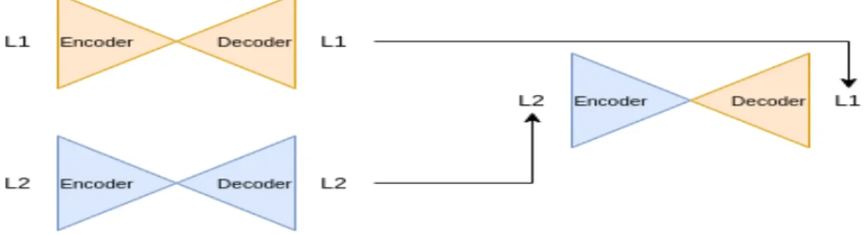
Figure 3.1: Representation of the phases of the autoencoder[35]

One thing that we should never forget, is the fact that, if we train two autoencoders separately, they are going to be incompatible with each other, because the latent face obtained in each one, will be based in specific features that each network “ marked” as meaningful during the training process, but if two autoencoders are separately trained on different faces, their latent spaces will represent different features. The thing that makes the swapping process possible is to find a way, where we force the two latent faces to be coded with the same features. We can solve this just by sharing the same encoder for each network, and different decoders.[35]

needs to be able to identify the features that are shared by both images. Once all the faces share a similar structure, it is not expected that the encoder learn the concept of the face itself.[35]

Figure 3.2: Representation of two different autoencoders that will focus on different features[35]

When all the training process is finished, we are going to start generating the deepfakes. if the network learns well what makes a face, the latent space will represent facial expressions and orientations.

To sum up, to have a good deepfake, we need to make sure that the two subjects that are fed as input, share as many similarities as possible, and in this way, we can be sure that the encoder that is shared between them can generalize the features. The image below represents the way a deepfake is formed:

Figure 3.3: Autoencoder deepfake creation scheme[35]

When we look at this process of creating deepfakes, we can see how it relates to what we are developing.

First, we can immediately see that they use autoencoders and what differs from our work is that they receive images instead of signals. In the first phase, they have an autoencoder that receives an image and tries to reconstruct it, following this idea, that’s how we started the development of our algorithm.

Second, they advance to the conversion part and for that, they create two autoencoders so that each one of them “learns” the most important features and change the decoders so that the image is converted. Again, and correspondingly this is how we did our conversions and in this way for the development of our conversion algorithm, we use some of the ideas present in these examples, which we will be described in more detail in the next chapter.

Methodology

This chapter is about the methodology of the thesis. In more detail, we are explaining the research approach, how we did the data collection, selection of samples, type of data, and the limitations of the project.

As already mentioned, this thesis aims at the creation of an algorithm to convert, electrocardiogram (ECG) signals from certain Leads into one target Lead. To achieve this goal, we purpose an algorithm to convert Leads with the help of deep learning techniques, such us, autoencoders.

4.1

Materials

The dataset used was PTB[5] and was obtained through physionet[14] (the research resource for complex physiologic signals) is a collection of ECG and has the following specifications:

• 16 input channels, (14 for ECGs, 1 for respiration, 1 for line voltage). • Input voltage: ±16 mV, compensated offset voltage up to ±300 mV. • Input resistance: 100Ω(DC).

• Resolution: 16 bit with 0.5 µV /LSB(2000 A/D units per mV). • Bandwith: 0-1 kHz (synchronous sampling of all channels).

• Noise voltage: max. 10 µV (pp), respectively 3µV (RMS) with input short circuit. 41

• Online recording of skin resistance.

• Noise level recording during signal collection.

The database contains 549 records from 290 subjects (aged 17 to 87, mean 57.2; 209 men, mean age 55.5, and 81 women, mean age 61.6; ages were not recorded for 1 female and 14 male subjects). Each subject is represented by one to five records. There are no subjects numbered 124, 132, 134, or 161. Each record includes 15 simultaneously measured signals: the conventional 12 Leads (i, ii, iii, avr, avl, avf, v1, v2, v3, v4, v5, v6) together with the 3 Frank Lead ECGs (vx, vy, vz). Each signal digitized at 1000 samples per second, with a 16-bit resolution over a range of ±16.384mV . On special request to the contributors of the database, recordings may be available at sampling rates up to 10 kHz.[5]

Within the header (.hea) file of most of these ECGs. The record is a detailed clinical summary, including age, gender, diagnosis, and where applicable, data on medical history, medication and interventions, coronary artery pathology, ventriculography, echocardiography, and hemodynamics. The clinical summary is not available for 22 subjects.[5]

As we mentioned before, the PTB database was retrieved from the physionet, that it is a repository that stores medical data. It was created to catalog biomedical research and offers access to large collections of data for free.[14]

4.2

Pre-processing

We chose this database because at the time it fills all the requisites we needed to start testing the autoencoder, the signals did not need a lot of modifications to be trained by the autoencoder.

Since we are working with fully-connected autoencoders and with convolutional au-toencoders, we got two different ways of pre-processing the same data.

4.3

Fully connected autoencoder

Starting with the fully-connected methodology, from the signal in the database, we only changed the way the signals were shown, that is, we got rid of background noise,

we also centered all signals in R to get them all normalized to be used later in the process. The approach we used for this task was applying a low-pass filter (a low-pass filter is used to remove the higher frequencies in a signal of data) which receives four arguments data (signals), cutoff (40), fs (1000) and order (5), combined with one high-pass filter (a high-high-pass filter is used to remove the higher frequencies in a signal of data), which receives four arguments data (signals), cutoff (1), fs (1000) and order (5), to get the entire signal clear, so it is easier for the algorithm to identify the R-peaks that will be used to center the signal. After being cleared, we used the Pan Tompkins algorithm to detect the R-peaks and stored all of them in an array (this algorithm detects fiducial points and is one of the most used. The way it processes is: it starts by reducing noise using filters and uses a derivative to extract information from the QRS complex. With the help of a quadratic function and a window that moves along the signal, it highlights the high frequencies and with an adaptive threshold it can detect the R peaks[27]), and this we used the implementation that was present in the package py-ecg-detectors[28], so when it is time to cut the signal we can easily find the place where to center the new window, that is going to be 0.25s earlier and 0.4s after the R-peak.

Once all signals, were centered, filtered and with the same size, we created a pickle file, to store all of them separating the data in two arrays, train and test, so when we moved to the autoencoder we only need to load the file instead of preform the task above explained every time.

4.4

Convolutional autoencoder

For the pre-processing of the convolutional autoencoder, it was much simpler, from the process described before the only thing we did was cutting the signal, but even that was easy just because for this one with did not need to find the R-peaks of the signal, we just cut the signals second by second. The way with did this was by creating a function (cut signal) that received 3 parameters the signal, and the measures we wanted for the new window. After cutting all the signals we just needed to reshape it in order to add the channel, so in this way, the autoencoder could train it.

Since we are organizing the data so that it can be trained by the autoencoder, it is necessary to divide it into two groups, training and testing, for that, we took the 549 readings and divide them so that we have 349 in the training group and 200 in the test group. After doing this division, we apply the transformations described above,

both for one and for the other.

4.5

Autoencoder

We moved on to create the autoencoder, that will perform the conversion. With the development of our search and implementation, we created four autoencoders. We started with the fully-connected than transform it so that it would give multiple outputs, this idea was done, so it would bring some improvement to what we already had. After having both of them working, and because we were always looking for ways to improve our results, it arose the idea of transform both of them into convolutional ones. In this section, we will be describing the way we did it.

4.5.1

Fully-connected

As was mention before, the first autoencoder we implemented, was the fully-connected one, which consisted of 9 Dense layers on the encoder part, 1 for the bottleneck, and 4 for the encode and decode part.

This autoencoder started to be just a “prediction machine”. This being, its main task was just to try and predict the Lead that was fed to the autoencoder as input. In this way, we had a better understanding of what the autoencoder was learning for each Lead. So in this part of training what we did was just changing the parameters, such as, number of the epochs, learning rates, optimizers, among others to seek the best combination.

When we felt we found a good combination we started to transform this “prediction machine” into a conversion one. For this to happen, in the previous step, when we were training the prediction, we end up with an autoencoder for each Lead we trained, so what we did was change the decoders, the same way we learn when we read about the deepfakes in the previous section, and start to give one Lead and try to convert into other.

The data fed to the autoencoder was a signal that was treated according to the pre-processing described above.

When the results were reflecting what we predict it should happen we move on to transform in a multi-output autoencoder.

4.5.2

Fully connected multi-output

We decided to improve our autoencoder so that instead of passing one Lead and converting to another, we pass one Lead and try to convert into several, this way we are with a more efficient, faster process and mainly one autoencoder will be sufficient to get all the views of the different Leads.

For the creation of this autoencoder, we took what we had already implemented and the change we made was, instead of just having a decoder, we now have one per Lead. To make what we are saying more visible we can observe our new autoencoder in the following diagram:

Figure 4.1: Autoencoder multi-output architecture

As you can see from the diagram, the process that will happen now will be, first, a Lead is fed to the autoencoder and that Lead will be converted into the others, in this case in Lead I, II, and III. To achieve this goal, what we did was to create an encoder that has the function of learning the main features of the Leads that we want to convert in, and then all the information that is gathered in the bottleneck instead of being given to just one decoder, it will be given to 3 and the different decoders will try to reconstruct the signal in each own Lead.

For that, and before we performed the training, it was necessary to reorganize the data, so that the conversion is carried out successfully. So what we did was, take the data and create a training vector (xtrain) that, in this case, has the 3 types of Leads, so in this way, the encoder can learn not only about one Lead but about as many Leads as the number of decoders and we also created a vector for each Lead (lead(n)) that has the same peak in the same position but of another Lead. To clarify what has been said, in practice what we have is the following: the first heartbeat of the xtrain is the one that has the peak R in Lead I in the 331’s sample. What will correspond to the 331 centered heartbeat in Lead II, and the heartbeat centered on Lead III and so on. These two will be the first heartbeats of Lead II and Lead III, respectively, and

the first heartbeat of xtrain will also be in the first position of Lead I (since it is from Lead I).

The architecture we defined for the multi-output autoencoder was: an input layer, 4 Dense layers on the encoder part, 1 for the bottleneck, and for each decoder we have 4 Dense layers and 1 output layer.

4.5.3

Convolutional autoencoder

After finishing the multi-output autoencoder, with changes in the parameters and the number of layers and seeing that the results were already what we expected, we decided not to let our goals stop there and so explore the creation of a convolutional autoencoder, basing this implementation on a UNet, with the change that instead of using 2D convolutional layers, we opted for 1D.

Before proceeding with the visualization of the results we obtained, let’s understand what a UNet is, it is a neural network that has a “U” architecture and as it happens in autoencoders it has two symmetrical parts. The left part, “contracting path”, where the convolutional process takes place and a right part, “expansive path”, made up of transposed convolutional layers.

The diagram below shows the network’s operation in a more intuitive way:

Figure 4.2: Representation of the UNet general architecture[19]

The image above represents the convolution process, where the green layers are the Conv1D and the red one is the max-pooling layer where the sample is downsized, our autoencoder is made by three of this combination of layers. After this process is done and the sample is in its smaller size we start the expansive path, where the sample is going to expand until the same size as the input.