Equity Valuation Using Accounting Numbers
on Internet and IT Service Firms
Nicole Torres Amaral
152414010
Advisor: José Correia Guedes
Dissertation submitted in fulfillment of requirements for the degree of Internatinal MSc in Finance at Católica-Lisbon School of Business and Economics,
1
Abstract
The development of the new economy and establishment of Internet-based companies created an industry of fast growing corporations with much interest to investors. The valuation of these firms has drifted away from estimates provided by traditional valuation models, which tend to undervalue Internet stocks consistently. Additionally, financial information has shown to be of little use when assessing the value of dot.com stocks (Trueman et al., 2001)
The objective of this paper is to shed some light on the usefulness of accounting-based valuation models when valuing Internet stocks. It attempts to provide users with a guide to the relative performance of models when valuing Internet companies and demonstrate how the assessment of these companies is compared to the valuation of firms in other industries.
Empirical results show that Internet and IT Service companies are harder to value, compared to other firms, using traditional valuation methods. The valuation model that provides the best estimates for these enterprises is the forward P/E calculated using a harmonic mean when compared to the RIVM and AEGM.
Results also show that analysts prefer stock-based valuation models to flow-based models.
2
Abstract
O desenvolvimento da nova economia e das empresas cujo negócio é realizado através da Internet deu aso à criação de uma industria de empresas com um crescimento extremamente acelerado de grande interesse para possíveis investidores. A avaliação de empresas ligadas á Internet afastou-se das estimativas que eram geradas usando os modelos tradicionais de avaliação de empresas, que a maioria das vezes subvalorizava consideravelmente as acções destas firmas. Adicionalmente, a informação financeira divulgada mostrou ser pouco útil para a avaliação das acções dot.com (Trueman et al., 2001).
O objective principal desta tese é identificar a utilidade dos modelos de avaliação baseados em relatórios financeiros na avaliação de empresas online. O intuito é facultar aos analistas um guia sobre a capacidade de estimação de alguns modelos na avaliação de empresas tecnológicas e comparar a precisão das estimativas para estas empresas com as estimativas do valor de outras empresas de diferentes indústrias.
Os resultados desta análise demonstram que as empresas tecnológicas são mais difíceis de estimar usando os modelos estudados. O P/E é identificado como o modelo que produz as melhores avaliações para estas empresas em comparação com o RIVM e o AEGM.
Os restados também mostram que os analistas preferem modelos que utilização informação relativa a empresas concorrentes versus os modelos que utilização as demonstrações de resultados das empresas.
3 Table of Contents
ABSTRACT 1
ABSTRACT 2
II. LIST OF TABLES 5
III. ABBREVIATIONS 6
1 INTRODUCTION 8
1.1 MOTIVATION 9
1.2 OUTLINE AND RESEARCH PROBLEM 10
2 LITERATURE REVIEW 11
2.1 INTRODUCTION 11
2.2 THE IMPORTANCE OF EQUITY VALUATION 11
2.3 USEFULNESS OF ACCOUNTING NUMBERS IN VALUATION 12
2.4 VALUATION MODELS 13
2.4.1 VALUATION PERSPECTIVES 13
2.4.2 STOCK-BASED VALUATION MODELS 14
2.4.3 FLOW-BASED VALUATION MODELS 18
2.5 VALUING INTERNET COMPANIES 24
2.6 EMPIRICAL EVIDENCE 25
2.6.1 EMPIRICAL EVIDENCE ON STOCK-BASED VALUATION MODELS 25
2.6.2 EMPIRICAL EVIDENCE ON FLOW-BASED MODELS 26
2.6.3 EMPIRICAL EVIDENCE ON RELATIVE PERFORMANCE 27
2.7 CONCLUDING REMARKS 29
3 LARGE SAMPLE ANALYSIS 30
3.1 INTRODUCTION 30
3.1.1 RESEARCH QUESTION AND PRIOR LITERATURE 30
3.1.2 HYPOTHESES DEVELOPMENT 32
3.2 RESEARCH DESIGN 33
3.2.1 DATA AND SAMPLE SELECTION 33
3.2.2 MODEL IMPLEMENTATION 36
4
3.3 DESCRIPTIVE STATISTICS 38
3.4 EMPIRICAL RESULTS 43
3.4.1 INTRA-SAMPLE ANALYSIS 43
3.4.2 CROSS-SAMPLE ANALYSIS 45
3.4.3 DIFFERENCES IN VALUATION ERRORS ACROSS VALUATION MODELS 46
3.4.4 EXPLANATORY POWER OF VALUATION MODELS 49
3.5 SUPPLEMENTARY ANALYSIS 51
3.6 CONCLUDING REMARKS 53
4 SMALL SAMPLE ANALYSIS 55
4.1 INTRODUCTION 55
4.1.1 RESEARCH QUESTION AND HYPOTHESIS DEVELOPMENT 55
4.2 RESEARCH DESIGN 56
4.2.1 DATA AND SAMPLE SELECTION 56
4.3 DESCRIPTIVE STATISTICS 58
4.4 EMPIRICAL RESULTS 59
4.4.1 DOMINANT MODEL ANALYSIS 59
4.5 CONCLUDING REMARKS 60
5 CONCLUSIONS 61
6 REFERENCES 62
7 APPENDIX 68
7.1 APPENDIX 1-DIVIDEND DISCOUNT MODEL VARIATIONS 68
7.2 APPENDIX 2-RIVM: ENTERPRISE PERSPECTIVE 68
7.3 APPENDIX 3-SAMPLE INDUSTRIES 69
7.4 APPENDIX 4-LARGE SAMPLE ANALYSIS VARIABLES 70
5
II. List of Tables
Table 1- Small Sample Supplementary Analysis Table 2- Analyst Forecast Periods
Table 3- Chi-Squared Test for Recommendations Table 4-Analyst Recommendations
Table 5- Chi-Squared Test for Dominant Model Table 6- Valuation Model Selection
Table 7- Report Descriptive Statistics Table 8- Company Descriptive Statistics Table 9- Brokers Included in Sample
Table 10- Sample Separation across Industries Table 11- Scenario Analysis
Table 12- Univariate Regressions Table 13- Test on Model Performance
Table 14- ANOVA Test on Model Performance for all Models Table 15- ANOVA analysis for cross-sample mean comparison Table 16- Test on Accuracy and Bias of Valuation Models Table 17- Descriptive Statistics for Valuation Model Errors Table 18- Descriptive Statistics for the Stocks
6
III. Abbreviations
AEGM- Abnormal Earnings Growth Model AIG- Abnormal Income Growth
CRSP- Centre for Research in Security Prices CSR- Clear surplus relation
DCF- Discounted Free Cash Flow Model DDM- Dividend Discount Model,
EBIT- Earnings before interest and tax
EBITDA- Earnings before interest, tax, depreciations and amortizations EBO- Edwards-Bell-Ohlson model
EMH- Efficient Market Hypothesis EPS- Earnings Per Share
EV-Enterprise Value
GAAP- Generally accepted accounting practices I/B/E/S- Institutional Broker’s Estimation System IITS- Internet and IT service companies
IPO-Initial public offering Ke- Cost of Equity
LTC- Low Tech Companies M&A-Mergers and acquisitions NAV-Net Asset Value
NI- Net income
NOA- net operating assets
NOPAT- Net operating profit after tax OIC- Other Industry Companies OHTC-Other High Tech Companies OLS- Ordinary Least Squares P/B- Price-to-Book
P/E- Price earnings Q1-1ST Quartile
7 R2- Explainability
RI-Residual Income
R&D- Research and Development
RIVM- Residual Income Valuation Model SD- Standard Deviation
SIC- Standard industry classification U.S.- United States of America
8
1 Introduction
The launch of the World Wide Web changed the world forever, not only by marking the lifestyle of an entire generation but by paving the way into the new economy that accompanied the dot.com bubble. The Internet played a major role in changing the structure of the world economy from a manufacturing rich market to a service-based economy where knowledge is highly valued.
Internet companies started to grow at an increasing rate, with young firms being enormously valued. Examples include Facebook that went public in 2012 as the second-largest IPO in the US of all time, reaching a market capitalization of over $100 billion on the first day (Russolillo, 2012). Also, Amazon and Microsoft are valued at $350 billion and $450 billion respectively and Whatsapp, a free messenger smartphone application with revenues of $10 million was sold for $22 billion.1
These companies are part of a significant industry of much interest to investors worldwide. Web-based social networks currently represent one of the fastest growing industries, with extreme market capitalizations (Klobucnik and Sievers, 2013). However, one problem subsists. With the introduction of this new industry came problems, in particular for investors who did not know how to value such a young market. Traditional valuation methods based on accounting numbers are constantly undervaluing stocks, and subjectivity became a large part of Internet stock valuation.
This issue persists today, with the increased level of intangible assets in these companies’ books and the significant growth rates, no consensus has been reached on the best way to value these firms.
1 Financial information was retreived from Bloomberg and are dated as of
9 We begin this study by defining an Internet company: “It is a company, whose majority or significant part of revenues is generated by the Internet or whose basic activity is based on a constant use of the Internet.” (Zarzecki, 2010)
1.1 Motivation
The question of how to value companies in such a relevant industry is what drives this research. Investors seem to believe that financial information is not sufficient to value these firms, and other factors should be introduced (Trueman et al., 2001).
Many believe that accounting numbers are not useful in valuing Internet stocks, although some academics believe that traditional methods are still relevant (Zarzechy, 2010).
The objective of this study is to shed some light on the usefulness of accounting valuation models and consequently accounting numbers. This paper will attempt to understand the relative performance of traditional valuation models such as price multiples and flow-based models.
An additional analysis will be based on analyst reports, to identify the use of these models and their ability to predict market prices.
This paper will not only attempt to gauge the usefulness of accounting valuation models, but it will also identify the best models and provide analysts with an idea of what model provides the best estimates.
The choice between different valuation models may seem arbitrary or related to the analysts' preferences or the information that he has available, but in fact, a proper estimation depends on their ability to identify the correct method, which is different for distinct types of firms. The choice of model will indeed involve a trade-off between cost and complexity.
10
1.2 Outline and Research Problem
This paper will start by identifying the relevant theory related to equity valuation using accounting numbers, specifying the most relevant valuation models. Model development, as well as implementation issues, will be described, followed by empirical evidence on relative performance.
The paper will then continue to analyse a large sample of firms, with the objective of answering the following question:
How do accounting valuation models perform when valuing Internet companies versus other firms?
Statistical tests along with regression analysis will be executed to establish the performance of valuation models.
Furthermore, a second analysis will be presented, on a smaller sample of firms, with the objective of understanding how analysts value companies, specifically Internet firms. This analysis will seek to identify what models analysts’ use and trends in their recommendations.
11
2 Literature Review
2.1 Introduction
This chapter will begin by describing the main research and theories on valuation using accounting numbers. Starting by recognizing the importance of equity valuation and the two perspectives used, followed by acknowledging the use of accounting numbers for valuation purposes. This section will then identify and illustrate the most relevant literature regarding valuation and will depict some theoretical models to build a solid understanding of the theory behind the analysis in the next chapter.
2.2 The Importance of Equity Valuation
What is equity valuation? Why is it important? If markets are efficient and securities correctly priced then why do analysts need to spend resources valuing stocks? These are questions that define the financial markets, as we know them. Equity valuation is an estimate of the present value of a stream of expected payoffs to shareholders; it implies looking into an “uncertain future” and making an “educated guess” (Lee, 1999). Although many theoretical models exist to assist analysts in the process of valuation, it remains a complicated procedure heavily reliant on the ability to forecast, subject to interpreter bias, which cannot be expected to deliver an absolute certainty (Damodaran, 2002). As Lee (1999) says eloquently, “valuation is as much art as it is science."
According to the efficient market hypothesis (EMH), stocks are efficiently priced, and markets react quickly to all available information in a rational way, leaving no opportunity for incremental gain to that obtained when an investor buys and holds a diversified portfolio (Malkier, 1989).
So why do we need equity valuation? Even if the market is efficient, there may be some degree of mispricing (Malkiel, 1989) resulting in differences between market value and the intrinsic value of a specific firm. Fundamental analysts who have the ability to identify the stock’s intrinsic value correctly can determine
12 if it is overvalued or undervalued to exploit the inefficiencies by buying or selling the specific stock. Also, sometimes there are assets for which there is no market value (for example when a firm is purchasing a department of the business and takes into account the synergies) and investors need to assess correctly the price they are willing to pay using valuation methods (Damodaran, 2002). Another practical use for valuation is provided to managers who are looking for ways to increase the value of their firm. Most business decisions involve evaluation, like capital budgeting, financing decisions, dividend policy and even credit risk analysis (Palepu, 1999). In conclusion, equity valuation is a fundamental pillar of the financial system and plays a vital role in many areas of finance, critical not only to the market equilibrium and individual investors looking to make a profit but also those interested in corporate finance.
2.3 Usefulness of Accounting Numbers in Valuation
The use of accounting numbers to investors is a crucial question that needs to be addressed initially to consequently review the validity of valuation models that incorporate accounting information, such as expected earnings, as an explanatory variable (Lev, 1989). Before determining the relevance of such valuation models, it is fundamental to identify whether accounting information is relevant to those who seek to evaluate firms. This subject has been a research area of high importance to many academics and has been extensively studied. The arguments against the use of earnings reports are mostly related to the fact that other sources reflect the same information, which reaches the market sooner. There are other ways to estimate the value of common stock without using earnings as an intermediate step (Beaver, 1968) and the correlation between earnings and returns is weak and unstable (Lev, 1989). Also, accounting earnings are thought to lack theoretical grounds required by rigorous economic analysis (Penman, 1992).
Ball and Brown (1968) performed an investigation on the variations of stock prices at the time income numbers were released, to identify if this information would have any impact on investors’ expectations regarding the firm's future
13 payoffs. By observing a high correlation between the sign of unexpected earnings and the sign of market variations (increase or decrease in stock price), their study revealed the usefulness of earnings reports to the capital markets. Beaver (1968) verified these results by demonstrating that earnings reports have information content, for both individual investors and the market equilibrium. The annual income numbers released in the report represent half of all the information published concerning a specific firm. However, most of it is predicted by the market in the preceding months to the release of the report (Ball and Brown, 1968).
2.4 Valuation Models
All accounting-based valuation models can be divided into two broad categories: Stock-based models (also known as multiples based) and flow-based models1.
The first group uses market information related to comparable firms to build an evaluation, while the second uses a large set of assumptions and estimates. This section will start by identifying the two perspectives of business valuation and will identify five primary valuation models, describing their elaboration along with implementation issues and advantages and disadvantages of using each model.
2.4.1 Valuation Perspectives
Most valuation methods can be structured in two ways. The first is to value only the equity of the firm -equity perspective and the second is to value the assets of the enterprise without taking into consideration the type of claims on such assets- entity perspective. Theoretically, both methods should produce the same estimate: The equity value (entity value) can be deduced from the entity perspective (equity perspective) by deducting (adding) the net debt of the firm (Palepu et. Al, 1999).
The equity perspective defined in equation (1) is more interesting for investors since it distinguishes amongst capital provided by shareholders and debt
14 holders providing a valuation that incorporates firm-specific financing decisions. 𝑆ℎ𝑎𝑟𝑒ℎ𝑜𝑙𝑑𝑒𝑟′ 𝑠 𝐸𝑞𝑢𝑖𝑡𝑦 = 𝑂𝑝𝑒𝑟𝑎𝑡𝑖𝑛𝑔 𝐸𝑛𝑡𝑖𝑡𝑦 − 𝑁𝑒𝑡 𝐷𝑒𝑏𝑡 (1) The entity perspective (equation (2)) values the total assets of the firm, ignoring financing decisions, which are not relevant to the value of the company, making this perspective more advantageous for the comparison of estimates from companies.
𝑂𝑝𝑒𝑟𝑎𝑡𝑖𝑛𝑔 𝐸𝑛𝑡𝑖𝑡𝑦 = 𝑆ℎ𝑎𝑟𝑒ℎ𝑜𝑙𝑑𝑒𝑟′ 𝑠 𝐸𝑞𝑢𝑖𝑡𝑦 + 𝑁𝑒𝑡 𝐷𝑒𝑏𝑡 (2)
2.4.2 Stock-Based Valuation Models
Stock-based valuation models also referred to as multiples valuation models, are very commonly included in financial analysts reports and investment bankers’ assessments due to their implied simplicity (Bhojraj Lee, 2002). These models have the ability to make reasonable estimates without recurring to multi-year forecasts and present value calculations, that characterize most flow based valuation methods (Liu et al., 2002).
Penman (2003) points out that this type of valuation uses the prices of comparable companies to extrapolate a price for the target, operating under the assumption that markets are efficient, and peer companies are priced correctly. Although multiples valuation uses a much simpler methodology, it shares the same underlying principles as the more sophisticated methods described in Section 2.4.3: value increases when future payoffs increase and decreases when risk increases and vice-versa (Liu et al., 2002).2
The usefulness of this method is extremely high when assessing private companies that do not have a market value, young companies with little historical records (Penman, 2003), IPO’s (Kim and Ritter, 1999), mergers and
2 Baker and Ruback (1999) also identify that multiples have incorporated an
implicit forecast of future payoffs and discount rate provided by current market required rates of return and industry growth rates.
15 acquisitions (Bhojraj Lee, 2002), and as a complement to more sophisticated valuations (Liu et al., 2002).
This model specifies the value of stock (Pit) by multiplying a selected value driver (𝑉𝐷𝑡) and the corresponding price multiple generated from a selection of
comparable companies (𝛽𝑖𝑡) demonstrated in equation (3):
𝑝𝑖𝑡 = 𝑉𝐷𝑡𝛽𝑖𝑡 (3)
The model presented in equation (3) can be improved by including an intercept that takes into account the effect of other variables other than the value driver. Nevertheless, the additional complexity introduced into the model exceeds the benefits of an improved estimation for models that use well-performing drivers (Liu et al., 2002).
The two perspectives of valuation defined previously can be predicted using stock-based valuation, by adapting the choice of value driver. For example, in a valuation of equity, a value driver such as net income should be chosen, while an assessment of the entity requires a value driver like the NOPAT.
The three steps needed to obtain an efficient estimate are (1) selecting an appropriate value driver, (2) choosing a group of comparable companies and (3) computing the benchmark multiple using the information provided by the group selected in the previous step (Palepu et al., 2010). These steps represent the implementation challenges of multiples models, and their execution is directly related to the performance of the model for each company.
Issues discussed in previous literature related to these steps are presented in the remainder of this section.
2.4.2.1 Selecting the Value Driver
Selecting an appropriate value driver is a crucial factor influencing the output of the multiples valuation model considerably and should be carefully analysed in the context of the asset being priced. An important feature of the multiples
16 analysis is that more than one value driver can be selected, by using a weighted average of various benchmark multiples (4):
𝑉𝑎𝑙𝑢𝑒 𝑜𝑓 𝑓𝑖𝑟𝑚 𝑖 = 𝑊1× 𝑉𝐷1,𝑖× 𝛽1+ 𝑊2× 𝑉𝐷2,𝑖× 𝛽2+ ⋯ + 𝑊𝑛× 𝑉𝐷𝑛,𝑖× 𝛽𝑛 (4) Where 𝑊𝑛 is the weights assigned to each value driver 𝑉𝐷𝑛,𝑖, and 𝛽𝑛 are the computed benchmark multiples.
This combined analysis can provide a superior estimate when merging drivers that are positively biased, such as earnings and negatively biased, like sales or asset multiples (Lee Lee, 2002).
Liu et al. (2002) studied the performance of various multiples based on enterprise value and found that forecasted earnings presented the lowest pricing errors, outperforming other multiples across most industries. His findings show that forward earnings are better that historical earnings and cash flows and book value of equity have a similar performance over sales which overall perform the worst.3
Various studies4 have identified that forecasted earnings are the best performing
multiple, with its performance enhancing with the increase of the forecast horizon.
As for cash flow multiples, Baker and Ruback (1999) and Lee Lee (2002) verify that using EBITDA over EBIT produces more accurate valuations.
2.4.2.2 Selecting Comparable Firms
The choice of similar companies should be based on the similarity in risk, profitability and growth among firms (Bhojraj Lee, 2002. However, this undertaking may present some exertions given that no two companies are equal.
3 Lee Lee (2002) also found that forecasts deliver enhanced results over
historical earnings, and sales provide the worst estimates.
4 Forecasted earnings accuracy are mentioned in Liu et al. (2002), Lee Lee
(2002), Kim and Ritter (1999), Bhojraj Lee (2002). Liu et al. (2007) show that forecasts improve estimates to a greater deal using earnings multiples.
17 In practice, enterprises in the same industry are used based on the assumption that these firms are expected to face the same level of risk and earnings growth as well as use similar accounting methods (Alford, 1992), factors that intensively affect valuation. The issue with selecting firms in the same industry is that there is the risk of a reduced assessment in the cases where the industries are not appropriately defined, and sub-groups of distinct companies are included (Alford 1992, Liu et al. 2002).
Liu et al. (2002) highlight in their paper that choosing comparable businesses that have similar earnings growth provides better valuations than merely picking random companies. Their findings are in line with Alford (1992) who identifies that valuation pricing errors decrease as firms are selected from a narrower SIC code of up to three digits.
Another systematic approach to selecting peer companies is presented by Bhojaj Lee (2002), who use regression analysis to create a "warranted multiple" and select comparable firms based on the proximity of their "warranted multiples" to that of the target company.
2.4.2.3 Computing the Benchmark Multiple
Choosing a method of multiples computation is of high importance given that distinct processes affect the valuation of the target firm, providing different estimates (Liu et al., 2002). The most popular methods for calculating benchmark multiples are described below:
𝑆𝑖𝑚𝑝𝑙𝑒 𝑀𝑒𝑎𝑛 =1𝑛× ∑ 𝑃𝑟𝑖𝑐𝑒𝑖 𝑉𝑎𝑙𝑢𝑒 𝐷𝑟𝑖𝑣𝑒𝑟𝑖 𝑛 𝑖=1 (5) 𝑉𝑎𝑙𝑢𝑒 − 𝑊𝑒𝑖𝑔ℎ𝑡𝑒𝑑 𝑀𝑒𝑎𝑛 = ∑𝑛𝑖=1𝑃𝑟𝑖𝑐𝑒𝑖 ∑𝑛𝑖=1𝑉𝑎𝑙𝑢𝑒 𝐷𝑟𝑖𝑣𝑒𝑟𝑖 (6) 𝑀𝑒𝑑𝑖𝑎𝑛 = 𝑀𝑖𝑑𝑑𝑙𝑒 𝑣𝑎𝑙𝑢𝑒 𝑏𝑒𝑡𝑤𝑒𝑒𝑛 𝑡ℎ𝑒 𝑜𝑏𝑠𝑒𝑟𝑣𝑒𝑑 𝑚𝑖𝑛𝑖𝑚𝑢𝑚 𝑎𝑛𝑑 𝑚𝑎𝑥𝑖𝑚𝑢𝑚 (7) 𝐻𝑎𝑟𝑚𝑜𝑛𝑖𝑐 𝑀𝑒𝑎𝑛 = (∑ 𝑉𝑎𝑙𝑢𝑒 𝐷𝑟𝑖𝑣𝑒𝑟𝑖 𝑃𝑟𝑖𝑐𝑒𝑖 𝑋 1 𝑛 𝑛 𝑖=1 ) −1 (8) Where n defines the total number of i comparable firms.
18 The use of the simple average can result in overestimations due to the existence of extreme values (Baker and Ruback, 1999)
Baker and Ruback (1999) and Liu et al. (2002) determine that the harmonic mean (8) is the best approach to calculating the benchmark multiple. It is calculated by averaging the inverted value driver and taking the inverse of that average.
In conclusion, stock-based models are very useful in situations such as IPO’s, M&A’s and valuing assets that do not have a market value and provide an easy and reliable estimate without having to recur to resource consuming forecasts of multi-period future payoffs. One drawback of this type of model is that it relies on the market to correctly price assets and can be subject to mispricing that disturbs the effectiveness of the estimates obtained.
2.4.3 Flow-Based Valuation Models
In this section, the most common direct valuation models will be discussed: Dividend Discount Model (DDM), Discounted Free Cash Flow Model (DCF), the Residual Income Valuation Model (RIVM) and the Abnormal Earnings Growth Model (AEGM). The main model assumptions, implementation formulas, issues, advantages, and shortcomings will be presented.
These models are all based on fundamental analysis and the assumption that the market value of a stock equals the present value of expected future payoffs (Francis et al., 2000). They construct valuation processes that can be divided into three segments: (1) forecasting of the valuation attribute up to time T; (2) forecasting the terminal value at time T; (3) estimating the cost of capital for the target firm (Courteau et al., 2006).
Theoretically, these models are expected to produce similar estimates (Lee 1999, Francis et al. 2000 and Courteau et al. 2006), but in practice, results differ due inconsistent forecasting properties, growth rates, and discount rates (Francis et al. 2000). Academics such as Lundholm and 0'Keefe (2001) find that such differences in results can be eliminated by the proper model implementation.
19
2.4.3.1 Dividend Discount Model
The discounted dividend model (DDM) defines the value of a firm’s equity as the sum of the discounted expected dividends paid to shareholders over the life of the company (Francis et al., 2000). The model originally developed by Williams (1938) is described in equation (9).
𝑉𝑡𝐷𝐷𝑀= ∑ 𝑑𝑡
(1+𝑟𝑒)𝑡
𝑇
𝑡=1 (9)
Where 𝑉𝐹𝐷𝐷𝑀 is the market value of equity at time t, 𝑑
𝑡 is the expected dividend
for year t, 𝑟𝑒 is the cost of equity capital and T is the expected life of the firm. In
this case, the terminal value is assumed to be the liquidating dividend (Francis et al., 2000). Although future dividends are uncertain, an alternative can be to use variations of this formula, assuming the firms pay a constant dividend or have a constant growth rate (Gordon et al. 1956).5 Precautions should be taken with
estimates from such models because results are highly influenced by the growth rate and therefore an incorrect input may cause deviated values (Damodoran, 2002).
Although this method is the simplest way to value stock (Damodoran, 2002), with variables that can be forecasted without many complications in the short term, it contradicts the proposition described in Modigliani Miller (1961) that states that dividend policy in period t has no effect on the price of that time. Also, by relating value to dividends, this model cannot be used for firms that do not pay dividends or that have arbitrary dividend policies (Penman, 2003).
Despite the model's shortcomings, the following models are derived from a particular specification of the DDM's terminal value (Penman, 1998).
5 The expected life of the enterprise is usually thought to be perpetual (T=∞).
20
2.4.3.2 Discounted Free Cash Flow Model
The discounted free cash flow (DCF) model is a variation of the DDM that substitutes dividends for free cash flows assuming that these are an improved proxy for value in the short term (Francis et al., 2000).
Free cash flow (𝐹𝐶𝐹𝑡) is defined as the cash available to the firm’s claimants after
all required investments are made (10):
𝐹𝐶𝐹𝑡 = (𝑆𝐴𝐿𝐸𝑆𝑡− 𝑂𝑃𝐸𝑋𝑡− 𝐷𝐸𝑃𝑡)(1 − 𝜏) + 𝐷𝐸𝑃𝑡− 𝑊𝐶𝑡− 𝐶𝐴𝑃𝐸𝑋𝑡 (10) Where for year t: 𝑂𝑃𝐸𝑋𝑡 are the operating expenses, 𝐷𝐸𝑃𝑡 are the depreciation
expenses, 𝜏 is the corporate tax rate, 𝑊𝐶𝑡 is the change in working capital and 𝐶𝐴𝑃𝐸𝑋𝑡 are the capital expenditures.
The intrinsic value of the firm (𝑉𝑡𝐹𝐶𝐹𝐹) is estimated by discounting 𝐹𝐶𝐹
𝑡 at the
business's cost of capital (𝑟𝑊𝐴𝐶𝐶)(equation 12). The shareholders' equity
(𝑉𝑡𝐹𝐶𝐹)(equation 11) is indirectly calculated6 By subtracting the claim of debt
holders (𝐷𝑡), other non-equity investors (𝑃𝑆𝑡) and excess cash and marketable securities (𝐸𝐶𝑀𝑆𝑡) (Copeland et al., 1994).
𝑉𝑡𝐹𝐶𝐹 = ∑ 𝐹𝐶𝐹𝑡 (1+𝑟𝑊𝐴𝐶𝐶)𝑡 𝑇 𝑡=1 + 𝐸𝐶𝑀𝑆𝑡− 𝐷𝑡− 𝑃𝑆𝑡 (11) with: 𝑟𝑊𝐴𝐶𝐶=𝜔𝐷(1 − 𝜏)𝑟𝑑+ 𝜔𝑃𝑆𝑟𝑝𝑠+ 𝜔𝐸𝑟𝑒 (12)
Where 𝜔𝐷 is the proportion of debt in the company’s capital structure, 𝜔𝐸 is the proportion of common equity, 𝜔𝑃𝑆 is the proportion of preferred stock,
𝑟𝑑, 𝑟𝑝𝑠 𝑎𝑛𝑑 𝑟𝑒 are the cost of debt, preferred stock and equity respectively.
6 𝑉
𝑡𝐹𝐶𝐹 but can be directly computed using the DCF model with operating cash
flows as an input. Both models lead to identical results if applied correctly (Copeland et al., 1994).
21 This method is preferred over the equity perspective calculation since corresponding equity cash flows with the correct cost of equity is exceptionally hard (Copeland et al., 1994).
In computing the 𝑉𝑡𝐹𝐶𝐹𝐹, a terminal value should be assumed to avoid infinite FCF
forecasts (Damodoran, 2002). Equation (13) defines the model with a growing perpetuity: 𝑉𝑡𝐹𝐶𝐹𝐹 = ∑ 𝐹𝐶𝐹𝑡 (1+𝑟𝑊𝐴𝐶𝐶)𝑡 𝑇 𝑡=1 +(𝑟𝐹𝐶𝐹𝑇+1 𝑊𝐴𝐶𝐶−𝑔) 𝑋 1 (1+𝑟𝑊𝐴𝐶𝐶)𝑇 (13)
In most circumstances, the DCF Model requires adjustments to convert analyst forecasts of earnings into FCFs, a process that implies an increased level of difficulty (Damodoran, 2002).
Since DCF assumes investment to decrease the value, this model can be problematic for profitable enterprises that have negative free cash flows for long periods of time (Penman and Sougiannis, 1998). The DCF model may not provide a good estimate of the firm's value since cash flows provide little understanding of the company's economic performance and profitability, as declining free FCF can hint reduced performance but also an investment for the future (Copeland et al., 1994).
2.4.3.3 Residual Income Valuation Model
The RIVM also referred to as the Edwards-Bell-Ohlson (EBO) valuation technique (Frankel and Lee, 1998), is a version of the dividend discount model (Lee Swaminathan, 1999). The model mentioned in Peasnell (1982) and developed in Ohlson (1995) and Feltham and Ohlson (1996) shifts the value analysis from the expected value of dividends. It uses the clear surplus relation (CSR) as an underlying assumption: all gains and losses affecting book value are also included in earnings (14) (O’Hanlon and Peasnell, 2002). Mathematically RIVM is initially described as (15):
22 𝑉𝑡𝑅𝐼𝑉𝑀 = ∑ 𝐸𝑡(𝑑𝑇+𝑖)
(1+𝑟𝑒)𝑖
∞
𝑖=1 (15)
Where 𝑉𝑡𝑅𝐼𝑉𝑀 is the stock’s value at time t, 𝐵
𝑡 is the book value of equity, 𝐸𝑡(𝑑𝑡+𝑖)
is the expected future dividend for the period t+i conditional on the information available at time t and 𝑟𝑒 is the cost of equity.
Assuming that the firm’s earnings and book value are forecasted under the CSR (Ohlson, 1995 and Feltham and Ohlson, 1996) (14), the estimate in equation (15) can be modified to assess the intrinsic value of the stock as a function of book value of equity plus an infinite sum of discounted residual income (Lee, 1999) (shown in equations 16a, 16b and 16d).
𝑉𝑡𝑅𝐼𝑉𝑀 = 𝐵𝑡+ ∑ 𝐸𝑡[𝑁𝐼𝑡+𝑖(1+𝑟−(𝑟𝑒𝐵𝑡+𝑖−1)] 𝑒)𝑖 ∞ 𝑖=1 (16a) 𝑉𝑡𝑅𝐼𝑉𝑀 = 𝐵 𝑡+ ∑ 𝐸𝑡[(𝑅𝑂𝐸𝑡+𝑖(1+𝑟−𝑟𝑒)𝐵𝑡+𝑖−1)] 𝑒)𝑖 ∞ 𝑖=1 (16b) 𝑅𝐼𝑡+𝑖 = 𝑁𝐼𝑡+𝑖 − (𝑟𝑒𝐵𝑡+𝑖−1) (16c) 𝑉𝑡𝑅𝐼𝑉𝑀 = 𝐵𝑡+ ∑ 𝐸(1+𝑟𝑡[𝑅𝐼𝑡+𝑖] 𝑒)𝑖 ∞ 𝑖=1 (16d)
Where NI is the firm’s net income, 𝑉𝑡𝑅𝐼𝑉𝑀 is the stock’s intrinsic value, 𝐸
𝑡 is the
expected value at time t, ROE is the after-tax return on book equity and 𝑟𝑒 is the required cost of capital assuming a flat term structure.7
This model separates company value into two factors: a measure of capital invested and the present value of all future wealth (Lee Swaminathan, 1999). In other words, it separates financing from operating activities (Feltham and Ohlson, 1996).
The RIVM produces an estimate equal to the book value of equity, if the firm does not create value and will generate approximations higher (lower) than 𝐵𝑡 if expected ROE is higher (lower) than 𝑟𝑒 (Lee Swaminathan, 1999).
23 This model may prove to be a useful tool in valuing companies given that estimates are not influenced by dividend policy or accounting standards (Francis et al., 2000). It also presents an advantage over the DCF models, as it treats investment as an asset and requires shorter forecasting horizons (Penman, 2003). Nevertheless, is it faced with implementation issues related to forecasting horizons, the cost of equity, terminal value calculations, corresponding book value to forecasts, earnings forecasts and dividend payout ratios (Lee Swaminathan, 1999). Another shortcoming of the model is while the RIVM uses forecasted financial statement numbers to value the firm (Ohlson, 1995), it does not link value to past reported figures (Lee,1999 and O’Hanlon and Peasnell, 2002).
Finally, the RIVM's reliance on the clear surplus relation and dependence on book values led Ohlson and Juetter-Nautoth (2005) to develop a variation of the model described next as the abnormal earnings growth model (AEGM).
2.4.3.4 Abnormal Earnings Growth Model
AEGM also referred to as the Ohlson and Juettner-Nauroth model is derived similarly to the RIVM, using the DDM. It conveys the intrinsic value of equity as the “capitalized next period expected earnings” plus the present value of the “capitalized forecast of abnormal earnings growth of subsequent years" (O'Hanlon, 2009). Abnormal earnings growth (equation 17) is defined as the difference between periodic earnings change and the standard return on the previous period retained earnings.
𝐴𝐸𝐺𝑡+1 = (𝐸𝑎𝑟𝑛𝑡+1− 𝐸𝑎𝑟𝑛𝑡) − (𝑟𝑒)𝑋(𝑅𝐸𝑡) (17)
The AEGM uses the capitalized expected subsequent period’s earnings (𝑦𝑡) as an anchor (equation 18), as opposed to the RIVM, which uses the book value of equity (O’Hanlon, 2009).
𝑦𝑡= 𝐸𝑎𝑟𝑛𝑡+1
24 Similarly to the RIVM derivation, the AEGM is obtained from the DDM, and its equity perspective is described in equations (19a), (19b) and (19c).
𝑉𝑡𝐴𝐸𝐺𝑀 =𝐸𝑎𝑟𝑛𝑡+1 𝑟𝑒 + ∑ (𝐸𝑎𝑟𝑛𝑡+1−𝐸𝑎𝑟𝑛𝑡)−(𝑟𝑒−1)𝑋(𝐸𝑎𝑟𝑛𝑡−𝑑𝑡) (1+𝑟𝑒)𝑡𝑟𝑒 ∞ 𝑡=1 (19a) 𝑉𝑡𝐴𝐸𝐺𝑀 =𝐸𝑎𝑟𝑛𝑟𝑡+1 𝑒 + ∑ 𝐴𝐸𝐺𝑡+1 (1+𝑟𝑒)𝑡𝑟𝑒 ∞ 𝑡=1 (19b) 𝑉𝑡𝐴𝐸𝐺𝑀 =𝐸𝑎𝑟𝑛𝑡+1 𝑟𝑒 + ∑ 𝐴𝐸𝐺𝑡+1 (1+𝑟𝑒)𝑡𝑟𝑒 𝑇 𝑡=1 +(1+𝑟𝐴𝐸𝐺𝑇+2 𝑒)𝑇𝑟𝑒(𝑟𝑒−𝑔) (19c)
AEGM presents advantages over the RIVM, as its inputs are a better estimate for market value (future earnings vs. book value of equity) and are better known by analysts (Ohlson, 2005). Also, forecasted changes in earnings need to be consistent with retained earnings between consecutive periods but do not have to follow the CSR.
In addition, the model presents an intuitively appealing formula, demonstrating how the current price depends on forward earnings and their growth, with no restrictions on dividend policy (Ohlson and Juettner-Nauroth, 2005).
2.5 Valuing Internet Companies
With the increased difficulty faced when valuing Internet companies using traditional valuation methods, many scholars look to alternative methods to estimates prices for such stocks. An alternative method to value internet companies was developed by S. Schwartz and Mark Moon (2000).
Schwartz and Moon (2000) argue that internet stock prices may not be the result of a market bubble, but in fact may possibly be rational prices if growth rates in revenues are high enough. The model uses real option theory and capital budgeting techniques depending on the estimation of a number of parameters, the most relevant being the revenues, expected growth rate of revenues, losses carried forward and cash balances. It is developed in continuous time with a discrete time approximation that enables users to estimate prices using annual or quarterly data, for example. The value of the firm is written as seen is equation (20).
25
𝑉 = 𝑉(𝑅, 𝜇, 𝐿, 𝑋, 𝑡) (20)
With R being the revenues, 𝜇 the expected growth in revenues, 𝐿 the loss carried forward, X the cash balances and t the time.
The model provides an explanation for the volatility and what seem to be unbelievably high stock prices, under the assumption that revenue growth rates are high and using well estimated parameters.
2.6 Empirical Evidence
2.6.1 Empirical Evidence on Stock-Based Valuation Models
Forward earnings measures with a broad forecast horizon are the best performing multiples over most industries, contradicting the idea that different industries use different multiples. Historical earnings, cash flow measures, the book value of equity and sales is the order of the performance of multiples after forward earnings (Liu et al., 2002).
Although sales are not a good performance measure in comparison to other value drivers, they are widely used to evaluate companies when earnings and cash flows are negative and in some emerging markets where earnings and cash-flows are perceived as uninformative (Liu et al., 2002)
Investors use cash flow multiples because they believe reported cash flows to be a good indication of future cash flows, which are less predisposed to management manipulation. (Liu et al., 2002)
When assessing the value of companies with weak but positive earnings, earnings based models should be avoided because these multiples give unrealistic low estimates (Lee Lee, 2002).
For enterprises that have a lot of intangible assets on their balance sheet and have much investment in R&D, earnings valuation models can produce numbers that notably underestimate their actual value. Since earnings are reduced despite
26 the fact that these companies' value is derived from uncertain future growth opportunities (Lee Lee, 2002).
Pricing errors are also the lowest when multiples are calculated using the harmonic mean and when comparable firms are not selected randomly (Liu et al., 2002).
The power of predictability of multiples valuation models varies positively with the increase in company size and profitability and is negatively correlated with the growth in value of intangible assets (Lee Lee, 2002) and the differences in accounting practices used by comparable companies Young and Zeng (2015). The fact that valuation results are more accurate for big businesses can be related to the fact that small enterprises have erratic earnings, and their value is derived from a small set of projects. (Lee Lee, 2002).
Given that these multiples use positive value drivers, these results may not be descriptive of firms reporting losses, start-up companies and growing businesses that have negative operating cash flows (Liu et al., 2002 and Liu et al. 2007). Dechow et al. (1999) agree that a simple forward P/E model adequately captures how investors determine the current price.
2.6.2 Empirical Evidence on Flow-Based Models
Francis et al. (2000) compared the reliability of the DDM, DCF, and AEGM and determined that in practice, AEGM's estimates are more accurate than those produced by the first two models.8 The explanation given for this phenomenon
was the ability of the latter model to incorporate both stocks (book value of equity) and flow components (abnormal earnings), while the other two models focus exclusively on flow factors. Frankel and Lee’s (1995) findings also support
8 Results show that the median absolute prediction error for AEGM, DCF and
DDM are 30%, 41%, and 69% respectively. AEGM value estimates explain 71% of the variation in current prices compared to 51% for DDM and 35% for FCF. These results are valid when distortions in book value are less that forecasting and measuring errors in discount and growth rates.
27 these results. Penman and Sougiannis (1998) find a similar relationship between models by testing the models with finite-horizon forecasts, identifying that forecasting accrual earnings and book values (RIVM) have practical advantages over forecasting dividends and cash flows (DDM and DCF model), specifically for companies that use GAAP.9
According to Francis et al. (2000) within the flow based model category, for companies with high R&D expenditures and significant accounting discretion, the best valuation is given by the AEGM.
Lundholm and O’Keefe (2001) find that analysis such as the previous ones are misguided since direct models are derived from the same underlying assumption and should present similar estimates. According to these authors, differences in estimates are usually due to three types of errors. The first is inconsistent forecasts, caused by starting the perpetuity with the wrong values. The second, an incorrect discount rate, is the result of a difference between the cost of equity used to evaluate investment directly, and the WACC used to assess equity through an entity perspective model. The third is missing cash flows, that is caused by calculating the valuation attributes in an inconsistent way, usually due to a breach of the CSR in the financial statement forecasts. Richardson Tinaikar (2004) compare the studies performed by Penman and Sougiannis (1998) and Lundholm and O'Keefe (2001) and find that the latter is correct when assuming that flow models should present the same estimates. They also give the previous credit for identifying that the DCF model requires extended periods of forecasted information and requires accrual information.
2.6.3 Empirical Evidence on Relative Performance
Multiples valuation, compared to flow-based models, have the advantage of using a simpler method to estimate stock prices. Although, unlike flow based models, they are based on the assumption that the market is correctly pricing assets and
9 In some circumstances GAAP allows for the breach of the clear surplus relation
28 are subject to the risk of the entire industry or group of firms being under or overvalued Kim and Ritter (1999).
According to Liu et al. (2002), forward earnings multiples perform better that intrinsic value measures based on residual income models, given the generic assumptions in calculating the terminal value in the latter model. Conflicting with their results, Courteau et al. (2006) finds that the direct methods outperform the forward P/E multiple models, using both pricing errors and return prediction tests, but admits that a combination of both models exceeds either method used on its own.
As for non-US companies, Ashbaugh and Olsoon (2002) find that earnings multiples provide better estimations compared to book value estimates and residual models.
Ultimately there is no consensus on which valuation model provides the best estimate. Therefore a mixture of stock-based models and flow-based models can be used to complement each other and provide a good understanding of the intrinsic value of the target asset.
29
2.7 Concluding Remarks
The previous chapter focused on identifying and exhibiting the most common equity valuation methods, shedding light on the advantages and disadvantages of the employment of each model.
Implementation issues for stock-based models are related to the choice of comparable companies, the multiple benchmark computation and the selection of value driver, while issues for direct methods are linked with forecasts, terminal value calculations and determining the required cost of capital.
Empirical evidence is presented on the performance of each model, with conflicting points of view regarding the best-performing estimate. Liu et al. (2002) identify forward earnings multiples as the best predictor of intrinsic value, while Courteau et al. (2006) believe that direct methods perform better. Within the multiples segment, forward earnings multiples computed using harmonic mean are recognised as the best predictor of value, while within the flow based models, the RIVM is perceived to outperform other models, though little analysis has been done on the performance of the AEGM.
The following chapter will be dedicated to the analysis of the theoretical models discussed here in a practical setting, observing specifically their performance when valuing Internet companies.
30
3 Large Sample Analysis
3.1 Introduction
This chapter is dedicated to testing some of the models described in the previous section on a large sample of firms with the aim of identifying their relative performance.
As previously mentioned, the focus of this paper is on the performance of accounting-based valuation models in producing estimates for Internet and IT Service companies (IITS companies). The aim is to understand the usefulness of these models in a fast growing industry characterized by an increased level of volatility and uncertainty. Many analysts and academics find that accounting information is of little use when valuing Internet stocks (Trueman et al., 2000). Such findings lead to the need for an analysis of the traditional methods of valuation for IITS firms, to shed some light on what methods should be used when valuing these companies.
The next sections will specify the research question undertaken in this study, hypothesis development, research design, some descriptive statistics of the data analysed and empirical results.
3.1.1 Research Question and Prior Literature
The process of valuing Internet companies has been of high importance since the formation of the dot-com bubble. These companies have proven to be extremely hard to value due to the reduced amount of historical financial information available on many IITS firms given the young age of the industry (Trueman et al., 2000). In addition to these factors, the industry has also shown signs of enormous growth and unpredictability, making it hard to look towards accounting numbers for guidance (Trueman et al., 2001 and Zarzecki, 2010). Unlike conventional firms, earnings are not priced in Internet stocks, and negative cash flows are seen as investments (Bartov et al., 2002), making it hard
31 to use accounting numbers as measures of value. These factors create little consensus on whether accounting based valuation models should be used to value Internet companies.
On one side, Hand (2000 and 2001) postulates that market values are strongly correlated with accounting data, though not linearly, arguing that revenues are the key driver of IITS stock prices. Zarzecki (2010) and Core et al. (2003) also find that traditional valuation models are still relevant in valuing these companies as long as appropriate assumptions are made, and estimations for probable scenarios are taken into account.
On the other hand, Amir and Lev (1996) find that firms with high levels of intangible assets (such as IITS) are seen by investors as companies with distorted earnings since value-boosting investments are treated as expenses, consequently leading them to look at non-financial information, as indicators of worth. A trending non-financial indicator in the IITS industry is web traffic, which is found to be correlated with market values and stock returns (Rajgopal and Venkatachalam, 2000 and Zarzecki, 2010).
This matter is of such importance that academics like Schwartz and Moon (2000) have developed a model to value Internet companies, based on real options theory and capital budgeting, which was tested by Klobucnik and Sievers (2013). Given this dichotomy, the essence of this study will be to identify the usefulness of accounting based models for the valuation of Internet and IT Service companies.
This section will not only attempt to determine the explanatory power of traditional valuation methods for IITS', but it will also seek to recognize the relative performance of stock-based and flow-based models. This dilemma is equally relevant. Theoretically, all models produce similar estimations (Lee 1999, Francis et al. 2000 and Courteau et al. 2006), but in practice, different assumptions are used and so each model produces a distinctive valuation. Additionally an attempt will be made on identifying if model performance is industry related.
32 The research question for this section is accordingly presented below:
Do P/E multiple, AEGM and RIVM perform worse in valuing the Internet and IT Service industry?
3.1.2 Hypotheses Development
Following the literature reviewed above, the following detailed hypotheses will be tested, in order to answer the broad research question
Hypothesis 1: Accounting based valuation models have lower accuracy and
greater negative bias when valuing Internet companies in comparison to firms in other industries.
Hypothesis 2: Valuation models have lower explanatory power when valuing
Internet companies.
Hypothesis 3: Stock-based models perform better than flow based models.
Hypothesis 4: Accounting based valuation models’ accuracy and bias varies
across industries.
Hypothesis 1 and 2 are similar in the way that they both test the usefulness of the studied valuation models for Internet companies. Hypothesis 1 observes whether or not the valuation models produce good estimates and compares results to those of other industries.
Hypothesis 2 explores to what extent the estimates produced, explain the variations in share prices observed. It is noted that to test this hypothesis, the estimates obtained for each model are regressed for towards the dependent variable that is defined as the share price in the April after the end of the fiscal year for each yearly observation. The findings of this research for both hypotheses are expected to be in line with the opinions of analysts and academics such as Schwartz and Moon (2000) who find that Internet stocks are hard to value using traditional methods.
33 Hypothesis 3 considers the relative performance of accounting-based valuation models. Comparing the bias, accuracy and explanatory power of each model will test this premise. Results are obtained through the use of hypothesis tests and regression analysis and are anticipated to favour the 2-year forward P/E multiple following the results of Liu et al. (2002).
Hypothesis 4 can be partially derived from the results obtained from the first two predictions. By comparing the estimates of each model between Internet companies and the other defined industries, an inference can be made on the difference among models for distinctive industries.
3.2 Research Design
This section will illustrate the sampling process undertaken to reach the four sub-samples required to test the defined hypotheses. Valuation model implementations will be recognized as well as all the relevant assumptions to answer the underlying research questions that were set out in the previous section.
The valuation models used in this chapter are the forecasted P/E multiple as the best representative of the stock-based models (Liu et al., 2002) the RIVM which is hypothesized to outperform stock-based models (Courteau et al., 2006) and the AEGM which is an improved version of the RIVM. All three models will be estimated using the equity perspective.
3.2.1 Data and Sample Selection
The original data set is comprised of accounting data, share prices and analyst forecasts for a sample of 6559 U.S. public firms between 2005 and 2013, adding up to a total of 33.552 firm-year observations.
34 Firm descriptive information and financial statement data are collected from Compustat®10, while analyst forecasts are retrieved from I/B/E/S and betas and
stock prices are obtained from CRSP.
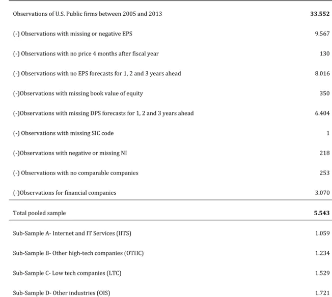
The sample selection process is described in Table 1 indicating the number of observations removed to get the foundations for solid statistical testing. Observations with missing information regarding variables that are necessary for the P/E, RIVM and AEGM valuations were removed, specifically missing current and forecasted EPS, the book value of equity, shares market value, dividends forecasts, and EPS growth rates. Observations that present negative values for net income and beta were excluded given that multiples valuations and cost of capital calculations require positive values for these variables. Financial companies were also excluded from the sample, in an attempt to create uniform sub-samples representing relatively similar industries.
The total sample remaining is of 5543 observations, which may include a single firm more than once. The sample is subsequently divided into four groups of industries: (1) the Internet and IT Services, (2) Other high-tech companies, (3) Low-tech businesses and (4) Other industries.
The definition of each sub-sample is based on studies performed by Francis and Schipper (1999), Kwon (2002) and Kwon et al. (2006). The former identify high and low tech industries based on the SIC codes of each company.11 In addition to
the SIC codes submitted by these authors, agricultural, mining and natural resource companies were added to the low-tech segment and manufacturing, and automobile companies were added to the high-tech group to obtain four segments with similar sample sizes. As for the Internet and IT Services industry, it is defined by Kile and Phillips (2009), that the industry is composed by eight 3-digit SIC codes. Other Industries represent the remainder of the sample.
10 Compustat values for the book value of equity per share and earnings per
share were adjusted for stock splits and dividends. I/B/E/S and CRSP data do not need adjustment.
35 Table 1- Sample selection process
Number of observations Observations of U.S. Public firms between 2005 and 2013 33.552
(-) Observations with missing or negative EPS 9.567
(-) Observations with no price 4 months after fiscal year 130 (-) Observations with no EPS forecasts for 1, 2 and 3 years ahead 8.016 (-)Observations with missing book value of equity 350 (-)Observations with missing DPS forecasts for 1, 2 and 3 years ahead 6.404
(-) Observations with missing SIC code 1
(-)Observations with negative or missing NI (-) Observations with no comparable companies
218 253
(-)Observations for financial companies 3.070
Total pooled sample 5.543
Sub-Sample A- Internet and IT Services (IITS) 1.059
Sub-Sample B- Other high-tech companies (OTHC) 1.234
Sub-Sample C- Low tech companies (LTC) 1.529
Sub-Sample D- Other industries (OIS) 1.721
Data was also retrieved from Bloomberg to calculate the risk-free and market return. The risk-free for each valuation year was obtained using the U.S 10 year treasury bonds and the market premium was computed using the yearly S&P returns from 1993 to 2013. The variables used in the large sample analysis are identified in Appendix 4.
36
3.2.2 Model Implementation
3.2.2.1 Stock-Based Valuation
The stock-based valuation model used is the 2-year forward P/E multiple, defined by Liu et al. (2002) as the best performing multiple. The estimate for the equity of a stock is computed by multiplying the value driver by the benchmark multiple.
The value driver used is the median analyst forecast of earnings per share two years ahead (EPS_2) and the benchmark multiple (Pmultiple) is calculated using a harmonic mean, for increased performance (Liu et al., 2002). Comparable companies (Ncomparables) are identified using the three digits SIC codes following the study performed by Alford (1992). To obtain better estimates, the target company is not included in the comparable group, and each firm is only accounted for once.
3.2.2.2 Flow-Based Valuation
Two flow-based models were selected, the RIVM and the AEGM. These evaluations were made as of April of the year after the fiscal year end for each observation and from an equity perspective.
The RIVM is derived using two periods, based on the median analyst forecast of earnings per share and a terminal value (21). Equity value is computed by adding the discounted residual incomes for the two periods(
RI_1
(1+Ke) for period 1 and
RI_2/(Ke−g))
(1+Ke) for period 2) to the book value per share
adjusted for stock splits and dividends (bjvlpsAJ). The choice of a two period model is due to the need of simplification and the fact that many observations do not have data for expected earnings 3-years ahead.
𝑉𝑡𝑅𝐼𝑉𝑀 = 𝑏𝑘𝑣𝑙𝑝𝑠𝐴𝐽 + 𝑅𝐼_1 (1+𝐾𝑒) +
𝑅𝐼_2/(𝐾𝑒−𝑔))
(1+𝐾𝑒) (21)
Where 𝑉𝑡𝑅𝐼𝑉𝑀is the equity value estimated using the RIVM, RI_1 and RI_2 are the
37 equity, and g is the growth rate. The AEGM was chosen, as it is theoretically an improvement of the RIVM (22). Estimates were originated using a two period model, with no perpetuity, as it is assumed that abnormal earnings in the long term will cease to exist given the competitiveness of the markets.
𝑉𝑡𝐴𝐸𝐺𝑀 =𝐸𝑃𝑆_1𝐾𝑒 +𝐾𝑒∗(1+𝐾𝑒)𝐴𝐸𝐺_1 +𝐾𝑒∗(1+𝐾𝑒)𝐴𝐸𝐺_2 2 (22)
Where 𝑉𝑡𝐴𝐸𝐺𝑀 is the equity value estimated using the RIVM, AEG are the
abnormal earnings for the period, EPS are the forecasted earnings per share for the next year and Ke is the cost of equity. Both models share the need for some assumptions such as the cost of capital, dividend payout rate and growth rates. As for the cost of equity (Ke), it was calculated using the CAPM formula (23). The inputs used were the risk-free rate (Rf), assumed to be equal to the U.S. 10 year Treasury bond rate of each year, the Market return (Rm), represented by the average S&P yearly returns over a period of 20 years and the equity betas are retrieved from CRSP
𝐾𝑒 = 𝑅𝑓+ 𝛽(𝑅𝑚− 𝑅𝑓) (23)
Additionally, the dividend payout rate, used to retrieve the residual income numbers was assumed to be equal to 1 in the cases where the current earnings per share were less than reported dividends. Similarly, valuations that resulted in a negative estimate were set to zero, as it is not economically viable to have negative equity. This was the case for 23 observations using the RIVM model and 170 using the AEGM.
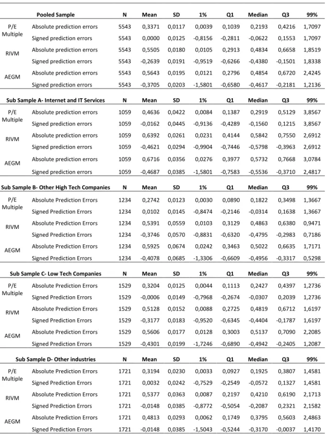
3.2.3 Performance Measures
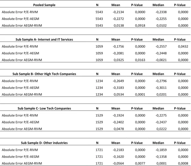
To assess the level of bias and accuracy of valuation models, the methodology employed in Liu et al. (2002), Lie and Lie (2002) and Corteau et al. (2007) will be implemented.
Valuation bias is assumed to be the model’s tendency to under- or overvalue a stock, measured by signed prediction errors (24).
38 𝑆𝑖𝑔𝑛𝑒𝑑 𝑃𝑟𝑒𝑑𝑖𝑐𝑡𝑖𝑜𝑛 𝐸𝑟𝑟𝑜𝑟𝑡 = 𝑉𝑡𝑚𝑜𝑑𝑒𝑙−𝑃𝑡
𝑃𝑡 (24)
Valuation accuracy is defined as the percentage of the stock’s price that is not incorporated in the value estimate, measured by absolute prediction errors (25). 𝐴𝑏𝑠𝑜𝑙𝑢𝑡𝑒 𝑃𝑟𝑒𝑑𝑖𝑐𝑡𝑖𝑜𝑛 𝐸𝑟𝑟𝑜𝑟𝑡 = |𝑉𝑡𝑚𝑜𝑑𝑒𝑙−𝑃𝑡|
𝑃𝑡 (25)
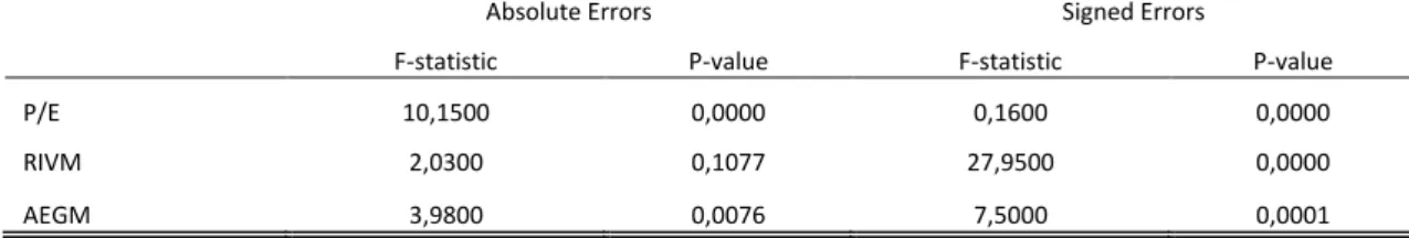
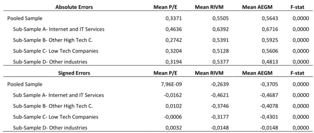
Absolute and signed errors are compared among models and industries using t-tests and Wilcoxon sign ranked t-tests for means and medians respectively.
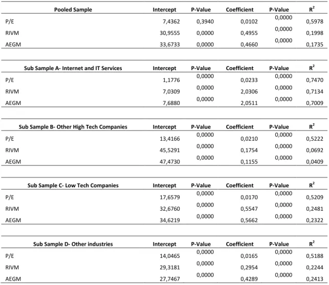
As for the explanatory power of each model, it will be identified through a linear regression using the price of the stock, at the valuation date, as an independent variable and the estimates derived from each model as an explanatory variable. The R2 of the regression will portray the percentage of variation of the
independent variable that is explained by the estimates.
The analysis of the research will be performed mostly regarding means and medians, with a higher emphasis on the latter, as it is seen as a more stable indicator (Damodoran, 2002).
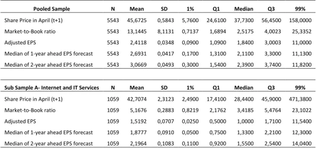
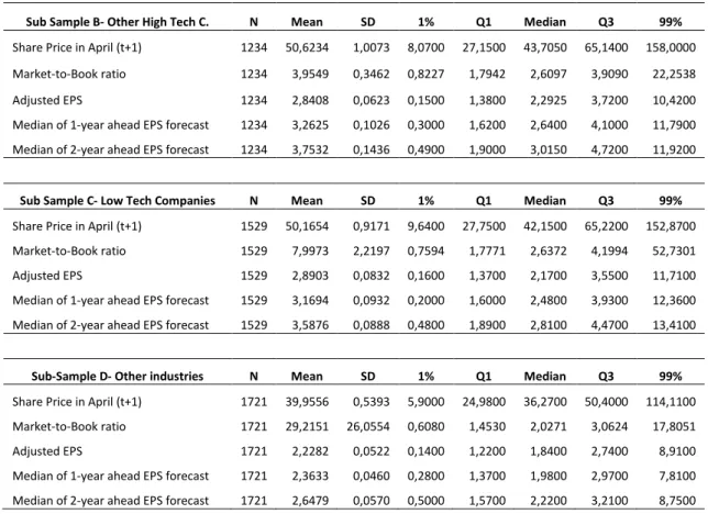
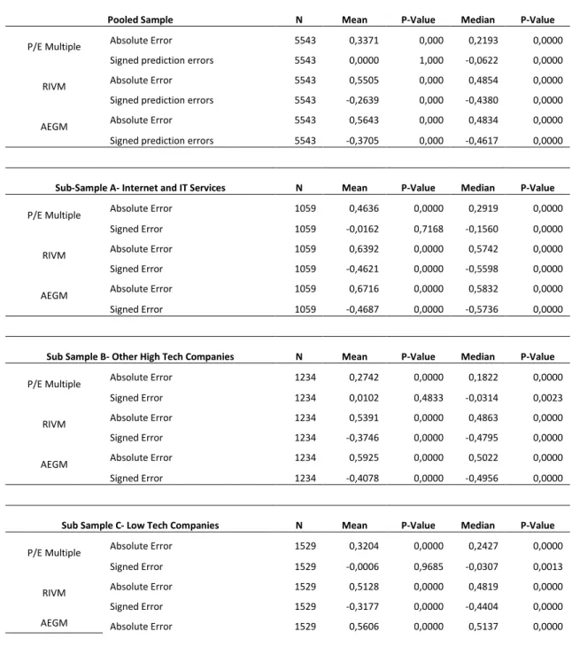
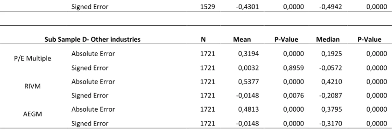
3.3 Descriptive Statistics
Table 2 and 3 identify the descriptive statistics for the pooled sample and selected subsamples. Table 2 provides information on the stocks included in the analysis while Table 3 focuses on the figures regarding the absolute and signed prediction errors.
The IITC sample has a standard deviation of 2,31, that when compared to the standard deviation of 1,00 for OHTC and 0,91 for LTC, it is noted that this sample has a larger dispersion of valuation errors, meaning that these companies are harder to value, compared to those in the other subsamples.
As for the Market-to-Book ratio, the median for IITC is above the median of the pooled sample indicating that investors expect these companies to create
39 more value given their current level of assets. This is common for stocks in this industry, given that a significant portion of their assets is intangible and may not be valued correctly or is expected to generate more future value than other firms with more traditional financial statements, such as manufacturing companies. Both current and forecasted earnings per share are reduced for IITC and OHTC, probably because the companies spend more on R&D and other investments that will create value in the long run, but are expensed in the current period. It is noted that the dispersion of earnings per share is also higher for Internet companies with 98% of observations ranging between 0,025 and 11,54 while OIC ranges between 0,5 and 8,75. This shows that not only do these companies have low earnings; they are more heterogeneous among peer firms. Given the high market-to-book ratio and the low level of earnings, results can be predicted to favour the hypothesis that earnings are less useful in valuing Internet stocks. In all samples, the means tend to be above the median values, indicating a degree of skewness, which may be a result of the restriction of the lower bound to zero for some variables, to eliminate negative equity valuations.
Table 2- Descriptive Statistics for the Stocks
Pooled Sample N Mean SD 1% Q1 Median Q3 99%
Share Price in April (t+1) 5543 45,6725 0,5843 5,7600 24,6100 37,7300 56,4500 158,0000 Market-to-Book ratio 5543 13,1445 8,1131 0,7137 1,6894 2,5175 4,0023 25,3352 Adjusted EPS 5543 2,4118 0,0348 0,0900 1,0900 1,8400 3,0003 11,0000 Median of 1-year ahead EPS forecast 5543 2,6931 0,0417 0,1700 1,3100 2,1100 3,3000 11,1300 Median of 2-year ahead EPS forecast 5543 3,0669 0,0493 0,3000 1,5400 2,3900 3,7400 11,8200
Sub Sample A- Internet and IT Services N Mean SD 1% Q1 Median Q3 99%
Share Price in April (t+1) 1059 42,7074 2,3123 2,4900 17,4100 28,4400 45,9000 471,3800 Market-to-Book ratio 1059 5,1676 0,2883 0,8219 2,1762 3,4185 5,4764 23,1022 Adjusted EPS 1059 1,5192 0,0707 0,0250 0,5000 1,0000 1,7100 11,5400 Median of 1-year ahead EPS forecast 1059 1,8777 0,0910 0,0500 0,7500 1,3300 2,2100 12,3000 Median of 2-year ahead EPS forecast 1059 2,1964 0,1083 0,1100 0,9200 1,5500 2,5400 14,0400